Spectral Approach to Plasma Kinetic Simulations Based on Hermite Decomposition in the Velocity Space

1. Introduction

Kinetic effects play a critical role in many problems in plasma physics. Correct description of kinetic processes typically requires solution of the Vlasov-Maxwell equations. Unfortunately, kinetic physics brings into the picture very small spatial (Debye length, electron gyroradius) and temporal (plasma frequency, electron gyrofrequency) scales, which could be several orders of magnitude smaller than system scales for most problems of interest. For example, in the Earth's magnetosphere the microscopic physics is key to magnetospheric dynamics during geomagnetic storms and substorms (Reeves et al., 2013; Jordanova et al., 2017). In the magnetosphere, the Debye length is of the order of ~ 1 − 100 m, while the system scales are ~10⁹ m. Similar or even more extreme separation of scales is typical of the solar wind and the solar corona, where kinetic physics is tied for example to mechanisms of energy release by magnetic reconnection and turbulence, impacting such fundamental problems as as the origin of coronal heating or solar wind heating and acceleration (e.g., Aschwanden, 2005; Bruno and Carbone, 2005). Despite remarkable recent progress in the development of efficient numerical methods for the solution of the Vlasov-Maxwell equations (for instance Chen et al., 2011; Markidis and Lapenta, 2011; Juno et al., 2018 and references therein), no existing fully-kinetic method appears capable of bridging the gap between microscopic and system scales given computational resources available now or in the foreseeable future.

Recognizing the inability of fully-kinetic methods to simulate large-scale systems, alternative approaches are being sought that focus on the so-called fluid-kinetic coupling. One line of research, appropriate in situation where kinetic effects are expected to be localized in space, seeks to embed a kinetic method in selected regions of a large-scale domain described by a fluid model (Sugiyama and Kusano, 2007; Kolobov and Arslanbekov, 2012; Daldorff et al., 2014; Tóth et al., 2016). For example, Particle-In-Cell (PIC) kinetic solvers have been successfully coupled to magnetohydrodynamics (MHD) large-scale solvers (Sugiyama and Kusano, 2007; Daldorff et al., 2014; Tóth et al., 2016). Another approach seeks extended fluid models by including high-order moments in the fluid hierarchy and seeking approximate closures capturing the physics of interest. Examples include the 5- and 10-moments methods discussed in Wang et al. (2015, 2018). Many other ideas on addressing fluid-kinetic coupling have been proposed in the literature (Markidis et al., 2014; Ho et al., unpublished¹). Furthermore, many well-established methods for solving Vlasov-Maxwell system, such as gyrokinetics (Brizard and Hahm, 2007), analytically remove certain spatial and temporal scales while retaining kinetic effects associated with larger/slower scales and thus may be suitable for certain class of problems involving fluid-kinetic coupling. However, despite the progress made, all of the existing methods have significant shortcomings and a comprehensive approach capable of obtaining accurate solutions in all parameters regimes remains elusive.

A new method for the solution of the Vlasov-Maxwell equations that could resolve the issues outlined above was recently proposed by Delzanno (2015). The method is based on a spectral discretization in velocity space and leads to a hierarchy of partial differential equations for the coefficients of the spectral expansion, akin to the moments of the fluid hierarchy. By a suitable choice of the spectral basis (in this case the asymmetrically-weighted Hermite functions), the low order moments of the expansion give a fluid description of the system. The kinetic physics is retained by adding more moments to the expansion. Thus, the fluid-kinetic coupling is an intrinsic feature of the method. One can immediately recognize that the method unifies and encompasses the fluid-kinetic approaches that have been described above. On the one hand, it can be seen as a reduced method that is not limited to any specific number of moments, but rather can be applied with as many moments as necessary for convergence, limited only by available computational resources. Furthermore, the number of moments could vary in the computational domain (even adaptively), in some analogy with kinetic-MHD-coupling approaches mentioned above. Significant advantage of the expansion method is that the transition between the “fluid” and “kinetic” regions can be as smooth as necessary. In all, spectral methods might offer on optimal way to perform large-scale simulations that include kinetic physics accurately.

In this paper, we describe a 3D parallel simulation code SpectralPlasmaSolver (SPS), which implements the method proposed in Delzanno (2015). The first application of the method to the problem of the three-dimensional turbulent cascade in the solar wind is demonstrated and the results are in good overall agreement with corresponding particle-in-cell simulations. The paper is organized as follows. In section 2 we briefly summarize the Hermite spectral method and its numerical formulation. In section 3, we discuss some aspects of the implementation, focusing on the parallelization for distributed-memory architectures. In section 4, linear properties of the methods and the simulations of decaying turbulence are discussed. Finally, a brief summary is presented in section 5.

2. Method

We consider Vlasov-Maxwell equations for the evolution of the distribution function f_s(x, v, t) of a collisionless, magnetized plasma consisting of electrons (labeled by subscript s = e) and singly-charged ions (s = i) in a three-dimensional Cartesian domain in physical space x. The three-dimensional velocity space is represented by v. The Vlasov equation reads:

$\begin{array}{cc}\frac{\partial f_s}{\partial t}+v·{\nabla }_x{f}_s+\frac{q_s}{e}\frac{{\Omega }_{cs}}{{\omega }_{pe}}\left(E+v\times B\right)·{\nabla }_v{f}_s=0,& (1)\end{array}$

where t is time, ∇_{x, (v)} represents the gradient operator in physical (velocity) space and E (B) is the electric (magnetic) field. Equation (1) is written according to the following normalization: time is normalized to inverse of the electron plasma frequency ω_pe computed with a reference plasma density n₀, ${\omega }_{pe}=\sqrt{\frac{e^2{n}_0}{{\epsilon }_0{m}_e}}$, where e is the positive elementary charge, m_s is the mass of species s, ε₀ is the permittivity of vacuum, t → ω_pet; velocities are normalized to the speed of light c, $\text{v}\to \frac{\text{v}}{c}$; spatial coordinates are normalized to the electron inertial length d_e = c/ω_pe, $\text{x}\to \frac{\text{x}}{d_e}$; the magnetic field is normalized to a reference magnetic field B₀, $\text{B}\to \frac{\text{B}}{B_0}$; the electric field is normalized to cB₀, $\text{E}\to \frac{\text{E}}{c{B}_0}$; and the distribution function is normalized to $\frac{n_0}{c^3}$, $f_s\to \frac{f_s{c}^3}{n_0}$. Furthermore, in Equation (1) q_s is the charge of each plasma species $\left(\frac{q_s}{e}=\pm 1\right)$ and ${\Omega }_{cs}=\frac{e{B}_0}{m_s}$ is the corresponding cyclotron frequency defined to be always positive. Equation (1) is coupled to Maxwell's equations by the electromagnetic field:

$\begin{array}{cc}\frac{\partial B}{\partial t}=-\nabla \times E,\frac{\partial E}{\partial t}=\nabla \times B-\frac{{\omega }_{pe}}{{\Omega }_{ce}}{\displaystyle \sum _s\frac{q_s}{e}}{\displaystyle \int v}{f}_{s}dv,& (2)\end{array}$

$\begin{array}{cc}\nabla ·E=\frac{{\omega }_{pe}}{{\Omega }_{ce}}{\displaystyle \sum _s\frac{q_s}{e}}{\displaystyle \int f_s}dv,\nabla ·B=0.& (3)\end{array}$

We assume periodic boundary conditions in physical space and consider domain [0, L_x] × [0, L_y] × [0, L_z]. The distribution function in velocity space is assumed to go to zero at infinity.

The Vlasov-Maxwell Equations (1)–(3) are solved with a spectral discretization in both physical and velocity space. In particular, we expand the distribution function as

$\begin{array}{l}{f}_s(x,v,t)={\displaystyle \sum _{k_x=-\frac{N_x}{2}}^{\frac{N_x}{2}}{\displaystyle \sum _{k_y=-\frac{N_y}{2}}^{\frac{N_y}{2}}{\displaystyle \sum _{k_z=-\frac{N_z}{2}}^{\frac{N_z}{2}}{\displaystyle \sum _{n=0}^{N_n-1}{\displaystyle \sum _{m=0}^{N_m-1}{\displaystyle \sum _{p=0}^{N_p-1}{C}_{n,m,p}^{k,s}}}}}}}(t)\\ \times {\eta }_{k_x}(x){\eta }_{k_y}(y){\eta }_{k_z}(z){\Psi }_n({\xi }_x^s){\Psi }_m({\xi }_y^s){\Psi }_p({\xi }_z^s),& (4)\end{array}$

with N_{x, y, z} (N_{n, m, p}) the number of modes in physical (velocity) space along each spatial direction. Here index k refers to a set of three indices k = {k_x, k_y, k_z}.

The electric field is expanded as

$\begin{array}{cc}E={\displaystyle \sum _{k_x=-\frac{N_x}{2}}^{\frac{N_x}{2}}}{\displaystyle \sum _{k_y=-\frac{N_y}{2}}^{\frac{N_y}{2}}}{\displaystyle \sum _{k_z=-\frac{N_z}{2}}^{\frac{N_z}{2}}}{E}^k(t){\eta }_{k_x}(x){\eta }_{k_y}(y){\eta }_{k_z}(z)& (5)\end{array}$

and similarly for the magnetic field B. We adopt a Fourier decomposition in physical space

$\begin{array}{cc}{\eta }_{k_{\delta }}(\delta )=\exp \left(\frac{2\pi i{k}_{\delta }\delta }{L_{\delta }}\right),& (6)\end{array}$

where δ = x, y, z. The decomposition in velocity space is obtained by asymmetrically-weighted (AW) Hermite basis functions, ${\text{Ψ}}_n(x)={(\pi 2^{n}n!)}^{-1/2}{H}_n(x)e^{-x^2}$, where H_n is the Hermite polynomial of the n-th order (Holloway, 1996). The argument of the basis functions is defined as ${\xi }_{\delta }^s=(v_{\delta }-u_{\delta }^s)/{\alpha }_{\delta }^s$, where $u_{\delta }^s$ and ${\alpha }_{\delta }^s$ are constant shift and scaling parameters. The method could also be formulated to allow spatial and/or temporal variations in $u_{\delta }^s$ and ${\alpha }_{\delta }^s$.

By substituting expansion (4) into Equations (1)–(3) and using the orthogonality relations for both Fourier and Hermite functions, we can rewrite the Vlasov-Maxwell equations as a system of non-linearly coupled ordinary differential equations (ODE) for the coefficients of the expansion. These are (Delzanno, 2015):

$\begin{array}{l}\frac{d{C}_{n,m,p}^{k,s}}{dt}=-\frac{2\pi i{k}_x}{L_x}{\alpha }_x^s\left(\sqrt{\frac{n+1}{2}}{C}_{n+1,m,p}^{k,s}+\sqrt{\frac{n}{2}}{C}_{n-1,m,p}^{k,s}+\frac{u_x^s}{{\alpha }_x^s}{C}_{n,m,p}^{k,s}\right)\\ -\frac{2\pi i{k}_y}{L_y}{\alpha }_y^s\left(\sqrt{\frac{m+1}{2}}{C}_{n,m+1,p}^{k,s}+\sqrt{\frac{m}{2}}{C}_{n,m-1,p}^{k,s}+\frac{u_y^s}{{\alpha }_y^s}{C}_{n,m,p}^{k,s}\right)\\ -\frac{2\pi i{k}_z}{L_z}{\alpha }_z^s\left(\sqrt{\frac{p+1}{2}}{C}_{n,m,p+1}^{k,s}+\sqrt{\frac{p}{2}}{C}_{n,m,p-1}^{k,s}+\frac{u_z^s}{{\alpha }_z^s}{C}_{n,m,p}^{k,s}\right)\\ +\frac{q_s}{e}\frac{{\Omega }_{cs}}{{\omega }_{pe}}\{\frac{\sqrt{2n}}{{\alpha }_x^s}{\left[E_x*C_{n-1,m,p}\right]}_k+\frac{\sqrt{2m}}{{\alpha }_y^s}{[E_y*C_{n,m-1,p}]}_k\\ +\frac{\sqrt{2p}}{{\alpha }_z^s}{[E_z*C_{n,m,p-1}]}_k\}+\frac{q_s}{e}\frac{{\Omega }_{cs}}{{\omega }_{pe}}[B_x*\{\sqrt{mp}\left(\frac{{\alpha }_z^s}{{\alpha }_y^s}-\frac{{\alpha }_y^s}{{\alpha }_z^s}\right)\\ \times C_{n,m-1,p-1}^s+\sqrt{m(p+1)}\frac{{\alpha }_z^s}{{\alpha }_y^s}{C}_{n,m-1,p+1^{-}}^s\\ \sqrt{(m+1)p}\frac{{\alpha }_y^s}{{\alpha }_z^s}{C}_{n,m+1,p-1}^s+\sqrt{2m}\frac{u_z^s}{{\alpha }_y^s}{C}_{n,m-1,p}^s\\ {-\sqrt{2p}\frac{u_y^s}{{\alpha }_z^s}{C}_{n,m,p-1}^s\}]}_k\\ +\frac{q_s}{e}\frac{{\Omega }_{cs}}{{\omega }_{pe}}[B_y*\{\sqrt{np}\left(\frac{{\alpha }_x^s}{{\alpha }_z^s}-\frac{{\alpha }_z^s}{{\alpha }_x^s}\right)C_{n-1,m,p-1}^s\\ +\sqrt{(n+1)p}\frac{{\alpha }_x^s}{{\alpha }_z^s}{C}_{n+1,m,p-1}^s-\sqrt{n(p+1)}\frac{{\alpha }_z^s}{{\alpha }_x^s}{C}_{n-1,m,p+1}^s\\ {+\sqrt{2p}\frac{u_x^s}{{\alpha }_z^s}{C}_{n,m,p-1}^s-\sqrt{2n}\frac{u_z^s}{{\alpha }_x^s}{C}_{n-1,m,p}^s\}]}_k\\ +\frac{q_s}{e}\frac{{\Omega }_{cs}}{{\omega }_{pe}}[B_z*\{\sqrt{nm}\left(\frac{{\alpha }_y^s}{{\alpha }_x^s}-\frac{{\alpha }_x^s}{{\alpha }_y^s}\right)C_{n-1,m-1,p}^s\\ +\sqrt{n(m+1)}\frac{{\alpha }_y^s}{{\alpha }_x^s}{C}_{n-1,m+1,p}^s-\sqrt{(n+1)m}\frac{{\alpha }_x^s}{{\alpha }_y^s}{C}_{n+1,m-1,p}^s\\ {+\sqrt{2n}\frac{u_y^s}{{\alpha }_x^s}{C}_{n-1,m,p}^s-\sqrt{2m}\frac{u_x^s}{{\alpha }_y^s}{C}_{n,m-1,p}^s\}]}_k,& (7)\end{array}$

for the Vlasov equation, and

$\begin{array}{l}\frac{d{B}_{\delta }^k}{dt}=-2\pi i{\epsilon }_{\beta \gamma \delta }\frac{k_{\beta }}{L_{\beta }}{E}_{\gamma }^k,\\ \frac{d{E}_{\delta }^k}{dt}=2\pi i{\epsilon }_{\beta \gamma \delta }\frac{k_{\beta }}{L_{\beta }}{B}_{\gamma }^k-\frac{{\omega }_{pe}}{{\Omega }_{ce}}{\displaystyle \sum _{s=e,i}\frac{q_s}{e}}{\alpha }_x^s{\alpha }_y^s{\alpha }_z^s\left(\frac{{\alpha }_{\delta }^s}{\sqrt{2}}{C}_{a,b,c}^{k,s}+u_{\delta }^s{C}_{0,0,0}^{k,s}\right)& (8)\end{array}$

for Maxwell's equations (written in index notation with summation over repeated indices implied). Here ε_βγδ is the Levi-Civita tensor and (a, b, c) = (1, 0, 0), (0, 1, 0), (0, 0, 1) for δ = x, y, z, respectively. Equations (7) are defined for n ∈ [0, N_n − 1], m ∈ [0, N_m − 1] and p ∈ [0, N_p − 1] and the convolution operator is defined as

$\begin{array}{cc}{\left[H*C_{n,m,p}\right]}_k={\displaystyle \sum _{k_x^{\prime }=-N_x/2}^{N_x/2}{\displaystyle \sum _{k_y^{\prime }=-N_y/2}^{N_y/2}{\displaystyle \sum _{k_z^{\prime }=-N_z/2}^{N_z/2}{H}^{k-k^{\prime }}}}}{C}_{n,m,p}^{k^{\prime },s},& (9)\end{array}$

where H is an arbitrary function. Note that Equation (7) couples a basis function (mode) indexed by n, m, p with successive modes of the hierarchy and it is necessary to specify how the system of equations is closed: We use $C_{n,m,p}^{\text{k},\text{s}}=0$ for n ≥ N_n, m ≥ N_m, p ≥ N_p. In order to address potential problems arising from the filamentation typical of collisionless plasmas, we add a collisional term on the right hand side of Eq. (7)

$\begin{array}{l}{C}[C_{n,m,p}^{k,s}]=-\nu [\frac{n(n-1)(n-2)}{(N_n-1)(N_n-2)(N_n-3)}\\ +\frac{m(m-1)(m-2)}{(N_m-1)(N_m-2)(N_m-3)}\\ +\frac{p(p-1)(p-2)}{(N_p-1)(N_p-2)(N_p-3)}]C_{n,m,p}^{k,s}.& (10)\end{array}$

The collisional operator given by Equation (10) is not meant to model any specific physical dissipation mechanism, such as Coulomb collisions. Rather, it is added to damp higher-order Hermite modes. This motivates the specific functional form of the operator, together with the requirement that it does not act on the first three modes of the Hermite expansion, which have connections to density, momentum and energy of the system (Delzanno, 2015; Camporeale et al., 2016). Other forms of the operator could be used to model Coulomb collisions or to provide a physically-inspired closure (Loureiro et al., 2016).

Equations (7) and (8) can be cast in matrix form as

$\begin{array}{l}\frac{dC}{dt}={\mathbb{L}}_{1}C+{N}\left(C,F\right),\\ \frac{dF}{dt}={\mathbb{L}}_{2}C+{\mathbb{L}}_{3}F,& (11)\end{array}$

where C represents the vector of $C_{n,m,p}^{k_x,k_y,k_z,s}$ coefficients and F contains the electric and magnetic field. Furthermore, L_1,2,3 represent the linear part of Equations (7) and (8) (advection in the case of Vlasov equations) while ${N}(\text{C},\text{F})$ represents the nonlinear part with the convolutions.

System (11) is discretized in time with a fully-implicit Crank-Nicolson scheme (Crank and Nicolson, 1947). In residual form, we have

$\begin{array}{cc}\{\begin{array}{l}{R}_1\left(C^{\theta +1},F^{\theta +1}\right)=C^{\theta +1}-C^{\theta }-\Delta t\left[{\mathbb{L}}_1{C}^{\theta +1/2}+{N}\left(C^{\theta +1/2},F^{\theta +1/2}\right)\right]=0\hfill \\ R_2\left(C^{\theta +1},F^{\theta +1}\right)=F^{\theta +1}-F^{\theta }-\Delta t{\mathbb{L}}_2{C}^{\theta +1/2}-\Delta t{\mathbb{L}}_3{F}^{\theta +1/2}=0\hfill \end{array}\iff ℝ(X)=0,& (12)\end{array}$

where Δt is the time step, and superscript θ labels time C(t^θ) = C(θΔt) = C^θ, and C^θ+1/2 = (C^θ+1+C^θ)/2 (and similarly for F), $X=\left[\begin{array}{c}C\\ F\end{array}\right]$ and $ℝ=\left[\begin{array}{c}{R}_1\\ R_2\end{array}\right]$.

The resulting numerical method formulated above and implemented in the SpectralPlasmaSolver (SPS) has several important properties. The main motivation for the choice of AW-Hermite spectral discretization of velocity space is the fact that the low order modes of the expansion correspond to the classic fluid description of the plasma (with a particular closure), while the kinetic physics is retained by adding more modes to the expansion. In other words, the fluid-kinetic coupling is an intrinsic feature of SPS. The Fourier discretization ensures that the constraints of Maxwell's equation (i.e., ∇·B = 0 and Poisson's equation) are automatically satisfied at all times if they are at t = 0. The fully-implicit Crank-Nicolson discretization improves the numerical stability of the method and ensures the exact conservation of total mass, momentum and energy in a finite time step. More details can be found in Delzanno (2015).

3. Implementation

The implementation of SPS described here extends 2D Fortran 90 code for shared-memory architectures that was described in Vencels et al. (2016). The new code implements full 3D algorithm described in section 2 and is parallelized for distributed memory architectures using Message Passing Interface (MPI) calls. Similarly to the previous implementation, the new code utilizes Jacobian-free Newton-Krylov solver provided by PETSc library (Balay et al., 1997, 2017). Since PETSc supports parallel computations with MPI, minimal modifications were required to parallelize the solver.

Computation of convolutions is based on a parallel Fast Fourier Transforms (FFTs). The code utilizes 1D and 2D domain decomposition of the solution space, such that each domain owns a portion of k-space for all fields and for all coefficients C. The parallel FFTs are implemented using a modified version of 2DECOMP&FFT library (Li and Laizet, 2010). Our modifications to 2DECOMP&FFT ensure that padding with zeros, necessary for performing convolutions, is performed in an efficient manner and zeros are never communicated between processors. In three dimensions, this results in significant reduction in overall computational cost of the 3D transform relative to directly padding the 3D array. FFTW library (Frigo and Johnson, 2005) or Intel MKL² (via its FFTW interface) can be used as the backend to compute FFTs.

Figure 1 shows examples of strong (top panel) and weak (bottom panel) scalings obtained on Blue Waters supercomputer. The strong scaling was obtained for a system with 255³ Fourier modes and N_h = 4 Hermite modes in each direction. The weak scaling study was performed by proportionally scaling up the system size and the MPI rank count for a system with 63³ Fourier modes and N_h = 4 Hermite modes per direction. These tests were performed on XE nodes of Blue Waters supercomputer and used 8 MPI ranks per node. GCC compilers version 4.9.3 and FFTW library version 3.3.4 were used to compile the code. Each Blue Waters XE node is equipped with 2 AMD Interlagos model 6276 CPU processors. Significant variability in timings for a given simulation size was observed in some tests, presumably due to how a particular job was placed with respect to the topology of the communication links. The results shown in Figure 1 represent the lowest value. The break point observed in both strong and weak scalings is most likely related to the fact that simulation time is limited by communication time at high rank count. This is further confirmed by results shown in Figure 2, which demonstrates strong scaling of SPS on Skylake nodes of Electra supercomputer at NASA Ames research center. Each Skylake node is equipped with two Xeon Gold 6148 processors. Intel compilers and MKL library version 110302 were utilized in these tests. Furthermore, mpiprof tool³ was used to collect separate timings for computation and MPI communication. The scaling shown here was obtained for a system with 255³ spatial modes, 4³ Hermite functions, and initial conditions corresponding to Maxwellian plasma. It is apparent that saturation of the overall scaling is related to increasing relative cost of the communication with increasing number of processes.

FIGURE 1

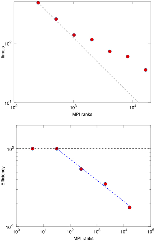
Figure 1. Examples of strong (Top) and weak (Bottom) scaling of SPS obtained on Blue Waters supercomputer. Dashed black lines denote ideal scalings. The efficiency of the weak scaling is defined as the ratio between the number of MPI ranks and simulation time normalized to that value for the reference case with 4 MPI ranks.

FIGURE 2

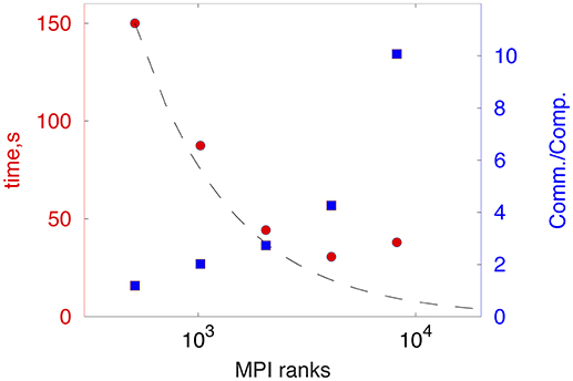
Figure 2. Example of strong scalings of SPS obtained on Electra supercomputer. Red circles represent computation time, blue squares mark the ratio of communication to computation time, and dashed lines denote ideal scalings.

These results point to a number of further enhancements in the code that would significantly increase parallelism and performance: (i) implementing decomposition in the Hermite coefficient space in addition to the k-space; (ii) overlapping communication and computation by using non-blocking collective MPI operations; (iii) performing transforms for several variables at a time.

4. Simulation of Kinetic Scales in Solar Wind Turbulence

Solar wind is believed to represent one of the best accessible examples of astrophysical large-scale plasma turbulence (Bruno and Carbone, 2005). The spectrum of magnetic fluctuations in the solar wind, as measured in-situ by spacecraft, exhibits power law behavior over many orders of magnitude in scales. A large range of scales, where fluctuations have predominantly Alfvenic character, exhibits many features expected of the inertial range of turbulence. This is followed by steepening to another power law range at proton kinetic scales kd_p ~ 1 (where d_p is the proton inertial length). The behavior at electron scales is less well characterized, but generally power law spectra are observed to extend to scales of the order of electron gyroradius, with subsequent steepening to either another power law or an exponential range reported in the literature (Sahraoui et al., 2010; Alexandrova et al., 2012).

In a classical paradigm of turbulence, the energy is transported by nonlinear interactions with no loss through the inertial range and is dissipated at small scales. In a weakly collisional plasma, such as solar wind, dissipation of the turbulent fluctuations is due to collective wave-particle interactions. These interactions can deposit the energy into various plasma components, such as thermal or suprathermal electrons, protons, and heavy ion species. Since turbulence has been proposed to play a significant role in the energy balance of solar wind, solar corona, and other space and astrophysical systems, understanding of the details of energy dissipation is a question of both significant theoretical interest and of great practical importance.

The problem of correctly describing energy dissipation in weakly collisional turbulence can be viewed as a problem of understanding fluid-kinetic coupling. Indeed, the fluctuations in the inertial range are widely thought to be well-described by MHD approximation. At the same time, adequate description of the dynamics at sub-proton scales and especially of the energy dissipation mechanisms requires electron and ion kinetic effects. The large-scale fluctuations drive dynamics at sub-proton scales, while the small-scale fluctuations may influence the large scales e.g., by supplying dissipation of energy and momentum, breaking topological constraints through magnetic reconnection, or placing constraints on values of temperature anisotropy enforced by instabilities. Significant progress has been achieved in numerical modeling of turbulence in weakly collisional plasmas (e.g., Howes, 2017), but the complexity of the problem drives interest in the methods capable of simulating sufficiently large range of scales, while describing kinetic effects with sufficient fidelity. In this section we describe an example of applying SPS to this problem. As the first step, we focus on the ability of the method to adequately describe kinetic dissipation and the small-scale dynamics.

4.1. Linear Dispersion Relation

Since the linear dispersion and damping of plasma modes are thought to be an important factor in determining the turbulence dynamics at sub-proton scales, we begin by discussing the ability of the Fourier-Hermite (FH) expansion approach to capture these properties for kinetic Alfvén wave (KAW). Observations in the solar wind and existing theoretical results suggest that KAWs play a significant, if not dominant role in the dynamics at sub-proton scales (e.g., Howes et al., 2008; Schekochihin et al., 2009; Salem et al., 2012; Chen et al., 2013). We note that linear properties of the Fourier-Hermite method, especially in the electrostatic limit, as well as its application to several other wave modes and instabilities are well described in the literature (e.g., Delzanno, 2015; Vencels et al., 2016 and references therein). The time-stepping formulation of the method is generally capable of following expected linear phase for a certain time, limited by recurrence. The accuracy of linear damping or growth rates increases with the number of Hermite basis functions. Furthermore, recurrence can be suppressed by including physical or artificial collision operator in the method formulation.

It is important to note that even when the number of Hermite basis functions is low (4–6 in each direction), the FH method can reproduce the linear properties of the waves with sufficient accuracy to yield an approximate model for sub-proton scale dynamics that compares well with fully kinetic PIC simulations (see section 4.2). Development of advanced fluid models targeting the sub-proton range of scales and capable of reproducing the damping rates of kinetic Alfvén and whistler modes has been the subject of intense research (e.g., Passot et al., 2017 and references therein). Such models typically rely on advanced closures, often incorporating expressions for the heat flux consistent with the linear theory (Hammett and Perkins, 1990). To make contact with the traditional fluid hierarchy, we first note that in asymmetrically-weighted formulation of the FH method an exact correspondence exists between the fluid moment equations and the evolution equations for coefficients of the expansion. Indeed, for any power r, v^r can be expressed

$\begin{array}{cc}{v}^r={\displaystyle \sum _{n\le r}{B}_n}{\Psi }^n(\xi ),& (13)\end{array}$

were B_n are constant coefficients, Ψⁿ is the dual Hermite basis function such that $\langle {\text{Ψ}}^m{\text{Ψ}}_n\rangle ={\delta }_{m,n}$, and 〈…〉 = ∫d³v(…). Then velocity moments of the kinetic equation can be related to the Hermite moments as

$\begin{array}{l}\langle v_x^p{v}_y^r{v}_z^l|{\partial }_t{f}_s+v·\nabla f_s+(\text{d}v/\text{d}t)·{\nabla }_v{f}_s\rangle \\ ={\displaystyle \sum _{m\le p}{\displaystyle \sum _{n\le r}{\displaystyle \sum _{p\le l}{B}_m}}}{B}_n{B}_p{\Psi }^m({\xi }_x){\Psi }^n({\xi }_y){\Psi }^p({\xi }_z)|{\partial }_t{f}_s+v·\nabla f_s\rangle \\ +\langle (\text{d}v/\text{d}t)·{\nabla }_v{f}_s.& (14)\end{array}$

For example, for N_m = N_n = N_p = 4, the system of evolution equations for coefficients C_{m, n, p} is equivalent to a fluid system that retains evolution equations for density, mean velocity, pressure, and heat flux tensors. The closure approximation relates the 4-th order moment to the lower ones using Equation (13). Remarkably, such a purely numerical closure can yield similar or better results than purposefully constructed models.

Here we focus on the (weakly damped) modes that are thought to be relevant to astrophysical turbulence. The ability of the method to describe some other modes and instabilities has been demonstrated in prior publications (e.g., Delzanno, 2015; Camporeale et al., 2016; Vencels et al., 2016). We present results from two complementary methods of analyzing linear properties of the method: decay of the initial perturbation in time-stepping context and the eigenvalues of the linearized equations. We consider uniform maxwellian plasma in a background magnetic field of strength B₀. The mass ratio is m_i/m_e = 100, ω_pe/Ω_ce = 2, and β_e = β_i = 0.5. Here ${\beta }_s=2{\mu }_0{n}_0{T}_s/B_0^2$ is the ratio between thermal pressure of species s and the magnetic pressure. The value of collisionality parameter in Equation 10 is ν = 0.01. The chosen ratio of ω_pe/Ω_ce is significantly lower than the one in many systems of interest, such as the solar wind, but is chosen to enable direct comparison with explicit PIC simulations (see section 4.2). The latter could not be conducted at realistic value of ω_pe/Ω_ce due to the requirement to resolve spatial scales of the order of Debye length ${\lambda }_e=(1/\sqrt{2})v_{th,e}/{\omega }_{pe}$ and temporal scales of the order of inverse plasma frequency. Here $v_{th,e}={(2T_e/m_e)}^{1/2}$ is the electron thermal speed. For example, the ratio of the ion inertial length to Debye length is $d_i/{\lambda }_e={(2{\beta }_e{m}_i/m_e)}^{1/2}{\omega }_{pe}/{\Omega }_{ce}$.

We consider angle of propagation θ = 88° with respect to the background magnetic field, as is characteristic of the kinetic Alfvén waves (KAW). For each value of k, Figure 3 shows the eigenvalue that is the closest to the KAW solution, as given by a linear Vlasov solver that implements equations of Stix (1992). As ν → 0, the imaginary part of eigenvalues tends to zero. However, for a range of values of ν, the imaginary part is weakly dependent on the collisionality and yields an approximation to collisionless damping rate obtained from the Vlasov solver accurate to 50% or better. It is important to emphasize that damping of a generic perturbation is the result of phase mixing between different eigenmodes and is thus better described in time-stepping formulation of the FH method (e.g., Grant and Feix, 1967). Figure 3 also includes real frequency and the damping rate obtained by initializing (fully nonlinear) SPS simulations with small-amplitude perturbation corresponding to eigenvector from the linear Vlasov solution. Overall, it is apparent that even when small number of Hermite modes is used, the method yields a good approximation to the collisionless damping rates and frequency for these nearly perpendicularly propagating modes. Such modes are the most relevant in the solar wind, since the turbulent cascade at both large and at the kinetic scales is highly anisotropic and supplies energy predominantly in the perpendicular direction (e.g., Goldreich and Sridhar, 1995; Schekochihin et al., 2009; Horbury et al., 2012).

FIGURE 3

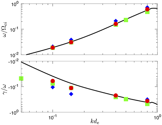
Figure 3. (Top) Frequency ω, corresponding to the real part of eigenvalues of linearized FH method or measured in time-stepping SPS simulations initialized with a small amplitude perturbation corresponding to KAW. (Bottom) The ratio of γ to ω, where γ is the imaginary part of the eigenvalue or the damping rate from the time-stepping solution. In all panels, blue and red symbols correspond to time-stepping simulations with N_h = 4 and N_h = 6 respectively, while green square correspond to eigenvalues computed for N_h = 6. The black curve shows numerical solution from a linear Vlasov solver. The angle of propagation is θ = 89°.

To provide more information on the linear properties of the method, Figures 4A–C show eigenvalues of the linearized algorithm for three different angles of propagation and several values of parameter N_h, the number of Hermite modes per direction. For each case, we show eigenvalues that are the closest to the Vlasov solution. Figure 4D shows the full spectrum of eigenvalues for the case N_h = 6, angle of propagation θ = 88°, kd_e = 0.5, and several values of the collisionality parameter ν. The latter plot illustrates the role played by finite collisionality: when ν is zero, all the eigenvalues are on the real axis and the solution corresponding to a damping mode in the linearized Vlasov equation is obtained as the result of phase-mixing between eigenmodes. With finite collisionality, the spectrum of eigenvalues becomes progressively sparser, but certain eigenvalues appear in the vicinity of the solution of the linearized Vlasov equation. It is those eigenvalues that give the solutions plotted in Figure 3. As the number of Hermite modes is increased for finite collisionality, the number of eigenvalues in the vicinity of the Vlasov solution increases (not shown).

FIGURE 4

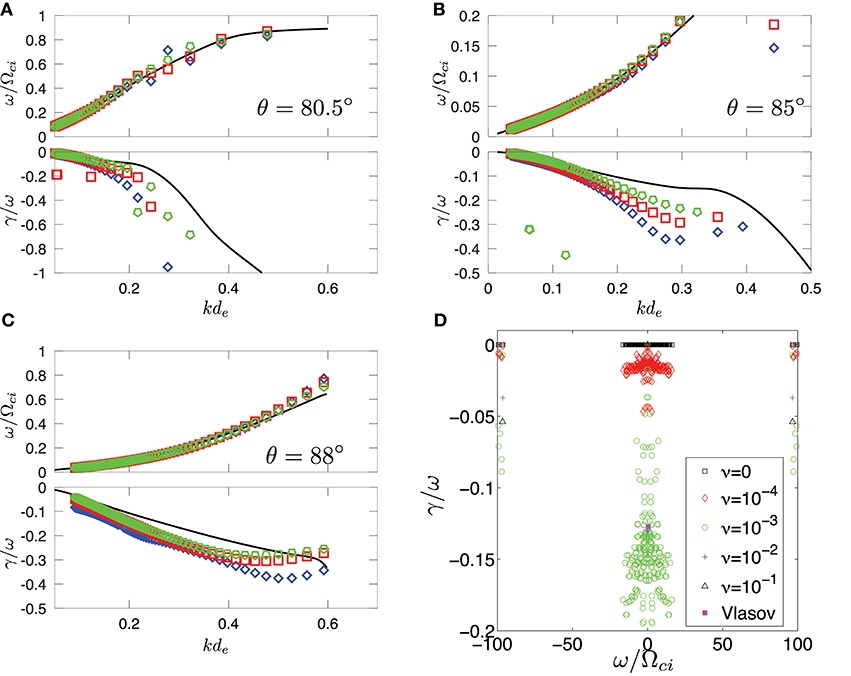
Figure 4. Eigenvalues of the linearized algorithm for the angle of propagation θ = 80.5°(A), θ = 85°(B), and θ = 88° (C). In (A) through (C), blue rhomb, red square, and green pentagon symbols refers to N_h = 4, 6, 8 respectively. (D) Shows the spectrum of eigenvalues for the case kd_e = 0.5, N_h = 6, θ = 88° and several values of the collisionality parameter ν.

4.2. Simulations of Decaying Turbulence

Having established that the FH method presented here is capable of adequately describing linear properties of the wave modes of interest, we present an example of a fully nonlinear simulation of turbulence targeting the physics at electron scales. We consider decaying turbulence, where no external forcing is applied and the turbulence develops as a result of the decay of an initial perturbation. The simulations are performed in an anisotropic rectangular simulation domain of size L_∥ = 400d_e and L_⊥ = 50d_e, where parallel and perpendicular refer to the orientation with respect to the background magnetic field. The simulation is initialized with Maxwellian uniform plasma and a perturbation of the magnetic field of the form $\delta \text{B}=\sum _k\delta {\text{B}}_{k}cos(k·x+{\psi }_k)$ and of ion flow $\delta V_i={\displaystyle {\sum }_k\delta V_k\cos (k·x+{\psi }_k)}$, where k = {p(2π/L_x), r(2π/L_y), l(2π/L_z)}, with p, r = −2…2 and l = 0…2. The amplitudes of the individual modes satisfy conditions k·δB_k = 0, B₀·δB_k = 0, k·δV_k = 0, and |δB_k| = |δV_k|. The mean energy ${{E}}_0$ of the initial perturbation is ${{E}}_0={\bar{{E}}}_0{L}_x{L}_y{L}_z{B}_0^2/(8\pi )$, where ${\bar{{E}}}_0=0.04$. The background plasma is characterized by β_e = 0.5 and ${\beta }_i=0.5-{\bar{{E}}}_0/3\approx 0.49$. The resolution in the Fourier space is 127 modes in each perpendicular direction and 31 modes in the parallel direction. We discuss two simulations with different numbers of Hermite basis modes in each direction for both electrons and ions, N_h = 6 and N_h = 5. The time step is $\Delta t=2{\omega }_{pe}^{-1}$ for the case with 5 Hermite modes and $\Delta t={\omega }_{pe}^{-1}$ for the case with 6 modes. The collisionality parameter in Equation (10) is ν = 0.01. In order to compare the SPS results with another well established technique for solving Vlasov-Maxwell system, we have conducted a Particle-In-Cell simulation of the same problem. The simulations utilized general-purpose code VPIC (Bowers et al., 2008) and used the same plasma parameters and similar, but not identical, initialization. The grid resolution in PIC simulation was 192 × 192 × 1600 cells, with time step $\Delta t\approx 0.15{\omega }_{pe}^{-1}$ and 10⁴ particles per cell per species at t = 0. The energy of the initial perturbation is lower than in SPS simulations ${\bar{{E}}}_0=0.02$.

Figure 5 summarizes some of the important statistical properties of fluctuations at the time tΩ_ci = 10 (when these properties become quasi-stationary) for the two SPS simulations and the PIC case. The top panel shows the spectrum of magnetic fluctuations $S_B(k)=\sum _{k_{\parallel }}\sum _{k<\left|k_{\perp }\right|<k+\delta k}|B(k){|}^2$. The spectrum appears to approach a power law at values kd_e ~ 1, where $S_B~k^{-3.8}$. However, due to very short range of scales considered, the power law behavior cannot be established reliably. In SPS simulations, a steepening is observed at scales between electron gyroradius ρ_e = v_{th, e}/Ω_ce and the Debye length λ_e, which are not well separated for the considered parameters since ${\rho }_e^2/{\lambda }_e^2=2{\omega }_{pe}^2/{\Omega }_{ce}^2$. This transition is followed by yet steeper spectrum at scales below Debye length, where fluctuations are essentially electrostatic. Overall, the spectra of magnetic fluctuations in SPS and PIC simulations are in good agreement, taking into account the lower energy of the initial perturbation in PIC. The only significant differences are observed at sub-Debye scales, similar to the results reported in Vencels et al. (2016). We note that PIC and SPS treat those scale differently. For example, grid effects strongly affect PIC results, while the presence of an explicit collisional operator may have a strong influence on the SPS results. We note however that in solar wind turbulence, majority of the cascading energy might be expected to be damped at scales kλ_e < 1. The saturation of the spectra in PIC simulations at high values of k is due to the numerical noise. Various techniques exist for mitigating effects of the noise in PIC simulations, such as spatial filtering or temporal averages (e.g., Wan et al., 2012; Roytershteyn et al., 2015). The PIC spectra shown here were averaged over 50 time steps, corresponding to time interval T_avΩ_ce≈3.6.

FIGURE 5

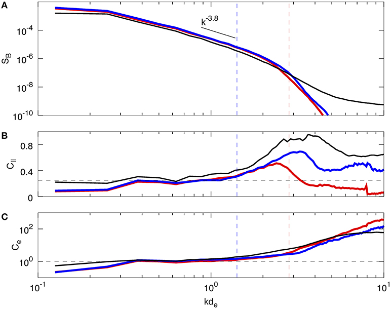
Figure 5. Spectrum of magnetic fluctuations (A), parallel compressibility (B), and electron compressibility (C) at tΩ_ci = 10. The vertical lines mark scales corresponding to kρ_e = 1 and kλ_e = 1. The horizontal lines in (B,C) mark values representative of KAWs. In all panels, the blue and red curves correspond to SPS simulations with N_h = 6 and N_h = 5 respectively. The black curves represent PIC simulation. The top panel also shows a characteristic local slope of the magnetic spectrum in the vicinity of kd_e ~ 1.

The middle panel of Figure 5 shows magnetic compressibility $C_{\parallel }=|\delta B_{\parallel }{|}^2/|\delta B{|}^2$, which has distinct values for different wave modes and is useful for identifying the origin of the observed fluctuations (Gary, 1993; Hollweg, 1999; Salem et al., 2012). In all of the simulations, the compressibility reaches values representative of kinetic Alfvén waves C_∥ = (1/2)β_i(1+τ)/[1+β_i(1+τ)] in the range $0.4/d_e\lesssim k\lesssim {\rho }_e^{-1}$, where τ = T_e/T_i (Boldyrev et al., 2013). However, C_∥ is about 15% higher in PIC simulations relative to both SPS cases in the range kρ_e ≲ 1. In all of the simulations, the compressibility increases after kρ_e ~ 1. The increase is somewhat sharper in PIC simulations and this behavior is better tracked by the N_h = 6 case. Finally, the bottom panel in Figure 5 shows another identifying signature of fluctuations, electron compressibility $C_e=(1/2){\beta }_i(1+\tau )\left[1+{\beta }_i(1+\tau )\right]|\delta n/n_0{|}^2/|\delta B/B_0{|}^2$. Again, in a significant range of scales kd_e ≲ 1 the properties of the fluctuations are consistent with KAWs. The values of electron compressibility in this range are very close between PIC and SPS simulations, but deviate at scales kρ_e≳1, with a sharper increase in the PIC case.

The properties of electron U_e and ion U_i velocity fluctuations are summarized in the top and bottom panels of Figure 6, respectively. At the sub-proton scales, the magnitude of electron velocity fluctuations significantly exceeds that of ions since ions are demagnetized. Overall, the behavior of |U_e| spectra is very similar to those of the magnetic field, with U_e spectra shallower by approximately k². A good agreement between PIC and SPS U_e spectra is seen at scales kλ_e ≲ 1. In contrast, the (weak) fluctuations of ion velocity exhibit more substantial differences between PIC and SPS cases. In particular, the PIC spectrum of U_i is shallower at small scales, leading to about a factor of 3 difference kd_e ~ 1, even though the overall energy of ion velocity fluctuations is lower in PIC.

FIGURE 6

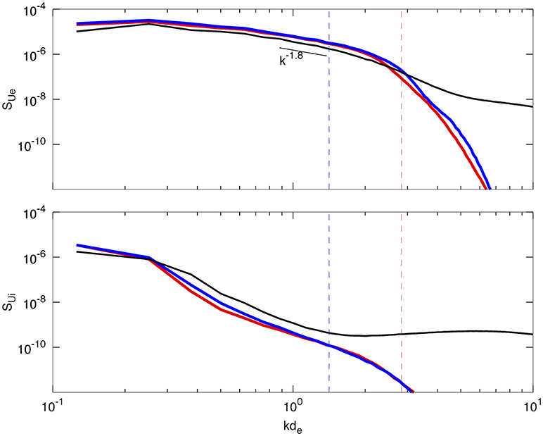
Figure 6. Spectra of electron (Top) and ion (Bottom) velocity fluctuations tΩ_ci = 10. The vertical lines mark scales corresponding to kρ_e = 1 and kλ_e = 1. In all panels, the blue and red curves correspond to SPS simulations with N_h = 6 and N_h = 5 respectively. The black curves represent PIC simulation. PIC spectra flatten out due to effects of numerical noise.

Finally, Figure 7 shows the evolution of the total energy in the simulations ${E}(t)$, normalized to the energy of the initial perturbation ${{E}}_0$. The SPS simulations, as expected, demonstrate excellent conservation properties (Delzanno, 2015). In fact, no change in the total energy is present within the accuracy of the diagnostic output. In contrast, PIC simulations exhibit noticeable numerical heating, which reaches the level of approximately 5% of the applied perturbation over the duration of the simulation. While this is likely acceptable for the present case, we had to use an unconventionally large number of particles to achieve such level of energy conservation.

FIGURE 7

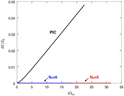
Figure 7. Energy conservation in the simulation of decaying turbulence. The curves show evolution of total energy ${E}$ in the simulation, which is the kinetic energy of plasma species plus the energy of the electromagnetic field, normalized to the energy of the initial perturbation $\delta {E}(t)=({E}(t)-{E}(0))/{{E}}_0$.

5. Summary

In this paper we summarized recent development of a highly parallelized version of the code SPS. SPS is a spectral code that implements dual Fourier-Hermite transform to obtain numerical solution of the Vlasov-Maxwell system. The method is particularly suitable for describing fluid-kinetic coupling since a direct analogy could be drawn between traditional fluid hierarchy and the equations for the evolution of the coefficients of expansion in the case of asymmetrically-weighted Hermite basis. In contrast to the traditional multi-moment models, the number of coefficients in the expansion is limited only by available computational resources, which opens up intriguing possibilities for building models capable of adaptively increasing the number of coefficients in selected regions of physical or wavenumber space.

As an example, we have discussed application of SPS to the problem of turbulence in weakly collisional plasmas. A model of plasma dynamics capable of capturing essential features of turbulence at electron scales could be obtained with only a few Hermite modes, as was demonstrated by considering linear properties of Kinetic Alfvén waves. Fully nonlinear simulations of decaying plasma turbulence were performed and successfully compared against corresponding PIC simulations. While some differences in the decay of the imposed perturbation of ion flow were observed between PIC and SPS, SPS simulations successfully reproduce most of the statistical properties of magnetic and electron fluctuations observed in PIC simulations at kρ_e ≲ 1. Significant differences in the spectra are observed at scales approaching Debye scale and below. In practice, this range of scales might not be significant for turbulence investigations, since most of cascading energy is expected to dissipate before it reaches Debye scales.

Data Availability Statement

The datasets for this study can be obtained by sending request to VR.

Author Contributions

VR and GLD closely collaborated on development and validation of the version of SPS discussed here and preparation of the manuscript.

Funding

This work was partially supported by NASA grant NNX15AR16G. GLD acknowledges funding by the Laboratory Directed Research and Development (LDRD) program, under the auspices of the National Nuclear Security Administration of the U.S. Department of Energy by Los Alamos National Laboratory, operated by Los Alamos National Security LLC under contract DE-AC52-06NA25396. Computational resources were provided by the NASA High-End Computing Program through the NASA Advanced Supercomputing Division at Ames Research Center. PIC simulations were conducted as a part of the Blue Waters sustained-petascale computing project, which is supported by the National Science Foundation (awards OCI-0725070 and ACI-1238993) and the state of Illinois. Blue Waters is a joint effort of the University of Illinois at Urbana-Champaign and its National Center for Supercomputing Applications. Blue Waters allocation was provided by the National Science Foundation through PRAC award 1614664.

Conflict of Interest Statement

The authors declare that the research was conducted in the absence of any commercial or financial relationships that could be construed as a potential conflict of interest.

Acknowledgments

We greatly acknowledge fruitful discussions on the physics of kinetic turbulence with S. Boldyrev. G. Jost analyzed our implementation of SPS and made a number of very useful recommendations for improving its performance.

Footnotes

1. ^Ho, A., Datta, I., and Shumlak, U. Physics-Based-Adaptive Plasma Model for High-Fidelity Numerical Simulations.

2. ^Intel^® Math Kernel Library. Available online at: https://software.intel.com/en-us/mkl

3. ^Jin, H. Using Mpiprof for Performance Analysis. Available online at: https://www.nas.nasa.gov/hecc/support/kb/using-mpiprof-for-performance-analysis_525.html

References

Alexandrova, O., Lacombe, C., Mangeney, A., Grappin, R., and Maksimovic, M. (2012). Solar wind turbulent spectrum at plasma kinetic scales. Astrophys. J. 760:121. doi: 10.1088/0004-637X/760/2/121

CrossRef Full Text | Google Scholar

Aschwanden, M. (2005). Physics of the Solar Corona. Springer Praxis Books. Berlin; Heidelberg: Springer.

Balay, S., Abhyankar, S., Adams, M. F., Brown, J., Brune, P., Buschelman, K., et al. (2017). PETSc Web Page. Available online at: http://www.mcs.anl.gov/petsc

Balay, S., Gropp, W. D., McInnes, L. C., and Smith, B. F. (1997). “Efficient management of parallelism in object-oriented numerical software libraries,” in Modern Software Tools for Scientific Computing, eds E. Arge, A. M. Bruaset, and H. P. Langtangen (Boston, MA: Birkhäuser Press), 163–202. doi: 10.1007/978-1-4612-1986-6_8

CrossRef Full Text | Google Scholar

Boldyrev, S., Horaites, K., Xia, Q., and Perez, J. C. (2013). Toward a theory of astrophysical plasma turbulence at subproton scales. Astrophys. J. 777:41. doi: 10.1088/0004-637X/777/1/41

CrossRef Full Text | Google Scholar

Bowers, K. J., Albright, B. J., Yin, L., Bergen, B., and Kwan, T. J. T. (2008). Ultrahigh performance three-dimensional electromagnetic relativistic kinetic plasma simulation. Phys. Plasmas 15:055703. doi: 10.1063/1.2840133

CrossRef Full Text | Google Scholar

Brizard, A. J., and Hahm, T. S. (2007). Foundations of nonlinear gyrokinetic theory. Rev. Mod. Phys. 79, 421–468. doi: 10.1103/RevModPhys.79.421

CrossRef Full Text | Google Scholar

Bruno, R., and Carbone, V. (2005). The solar wind as a turbulence laboratory. Living Rev. Solar Phys. 2:4. doi: 10.12942/lrsp-2005-4

CrossRef Full Text | Google Scholar

Camporeale, E., Delzanno, G., Bergen, B., and Moulton, J. (2016). On the velocity space discretization for the Vlasov-Poisson system: comparison between implicit Hermite spectral and Particle-in-Cell methods. Comput. Phys. Commun. 198, 47–58. doi: 10.1016/j.cpc.2015.09.002

CrossRef Full Text | Google Scholar

Chen, C. H., Boldyrev, S., Xia, Q., and Perez, J. C. (2013). Nature of subproton scale turbulence in the solar wind. Phys. Rev. Lett. 110, 1–5. doi: 10.1103/PhysRevLett.110.225002

PubMed Abstract | CrossRef Full Text | Google Scholar

Chen, G., Chacon, L., and Barnes, D. C. (2011). An energy- and charge-conserving, implicit, electrostatic particle-in-cell algorithm. J. Comput. Phys. 230, 7018–7036. doi: 10.1016/j.jcp.2011.05.031

CrossRef Full Text | Google Scholar

Crank, J., and Nicolson, P. (1947). A practical method for numerical evaluation of solutions of partial differential equations of the heat-conduction type. Math. Proc. Cambridge Philos. Soc. 43, 50–67. doi: 10.1017/S0305004100023197

CrossRef Full Text | Google Scholar

Daldorff, L. K. S., Tóth, G., Gombosi, T. I., Lapenta, G., Amaya, J., Markidis, S., et al. (2014). Two-way coupling of a global Hall magnetohydrodynamics model with a local implicit particle-in-cell model. J. Comput. Phys. 268, 236–254. doi: 10.1016/j.jcp.2014.03.009

CrossRef Full Text | Google Scholar

Delzanno, G. (2015). Multi-dimensional, fully-implicit, spectral method for the Vlasov-Maxwell equations with exact conservation laws in discrete form. J. Comput. Phys. 301, 338–356. doi: 10.1016/j.jcp.2015.07.028

CrossRef Full Text | Google Scholar

Frigo, M., and Johnson, S. G. (2005). The design and implementation of FFTW3. Proc. IEEE 93, 216–231. doi: 10.1109/JPROC.2004.840301

CrossRef Full Text | Google Scholar

Gary, S. P. (1993). Theory of Space Plasma Microinstabilities. Cambridge: Cambridge University Press.

Google Scholar

Goldreich, P., and Sridhar, S. (1995). Toward a theory of interstellar turbulence. 2: strong alfvenic turbulence. Astrophys. J. 438:763.

Google Scholar

Grant, F. C., and Feix, M. C. (1967). Fourier-hermite solutions of the Vlasov equations in the linearized limit. Phys. Fluids 10, 696–702. doi: 10.1063/1.1762177

CrossRef Full Text | Google Scholar

Hammett, G. W., and Perkins, F. W. (1990). Fluid moment models for Landau damping with application to the ion-temperature-gradient instability. Phys. Rev. Lett. 64, 3019–3022. doi: 10.1103/PhysRevLett.64.3019

PubMed Abstract | CrossRef Full Text | Google Scholar

Holloway, J. P. (1996). Spectral velocity discretizations for the vlasov-maxwell equations. Transp. Theory Stat. Phys. 25, 1–32. doi: 10.1080/00411459608204828

CrossRef Full Text | Google Scholar

Hollweg, J. V. (1999). Kinetic Alfvén wave revisited. J. Geophys. Res. Space Phys. 104, 14811–14819. doi: 10.1029/1998JA900132

CrossRef Full Text | Google Scholar

Horbury, T. S., Wicks, R. T., and Chen, C. H. K. (2012). Anisotropy in space plasma turbulence: solar wind observations. Space Sci. Rev. 172, 325–342. doi: 10.1007/s11214-011-9821-9

CrossRef Full Text | Google Scholar

Howes, G. G. (2017). A prospectus on kinetic heliophysics. Phys. Plasmas 24:055907. doi: 10.1063/1.4983993

PubMed Abstract | CrossRef Full Text | Google Scholar

Howes, G. G., Cowley, S. C., Dorland, W., Hammett, G. W., Quataert, E., and Schekochihin, A. A. (2008). A model of turbulence in magnetized plasmas: implications for the dissipation range in the solar wind. J. Geophys. Res. 113:5103. doi: 10.1029/2007JA012665

CrossRef Full Text | Google Scholar

Jordanova, V., Delzanno, G., Henderson, M., Godinez, H., Jeffery, C., Lawrence, E., et al. (2017). Specification of the near-earth space environment with shields. J. Atmospher. Solar Terrestr. Phys. doi: 10.1016/j.jastp.2017.11.006. [Epub ahead of print].

CrossRef Full Text | Google Scholar

Juno, J., Hakim, A., TenBarge, J., Shi, E., and Dorland, W. (2018). Discontinuous Galerkin algorithms for fully kinetic plasmas. J. Comput. Phys. 353, 110–147. doi: 10.1016/j.jcp.2017.10.009

CrossRef Full Text | Google Scholar

Kolobov, V., and Arslanbekov, R. (2012). Towards adaptive kinetic-fluid simulations of weakly ionized plasmas. J. Comput. Phys. 231, 839–869. doi: 10.1016/j.jcp.2011.05.036

CrossRef Full Text | Google Scholar

Li, N., and Laizet, S. (2010). “2decomp&fft — a highly scalable 2d decomposition library and fft interface,” in Cray User Group 2010 Conference (Edinburgh, UK).

Google Scholar

Loureiro, N. F., Dorland, W., Fazendeiro, L., Kanekar, A., Mallet, A., Vilelas, M. S., et al. (2016). Viriato: a Fourier-Hermite spectral code for strongly magnetized fluid-kinetic plasma dynamics. Comput. Phys. Commun. 206, 45–63. doi: 10.1016/j.cpc.2016.05.004

CrossRef Full Text | Google Scholar

Markidis, S., Henri, P., Lapenta, J., Rönnmark, K., Hamrin, M., Meliani, Z., et al. (2014). The fluid-kinetic Particle-in-Cell method for plasma simulations. J. Comput. Phys. 271, 415–429. doi: 10.1016/j.jcp.2014.02.002

CrossRef Full Text | Google Scholar

Markidis, S., and Lapenta, G. (2011). The energy conserving particle-in-cell method. J. Comput. Phys. 230, 7037–7052. doi: 10.1016/j.jcp.2011.05.033

CrossRef Full Text | Google Scholar

Passot, T., Sulem, P. L., and Tassi, E. (2017). Electron-scale reduced fluid models with gyroviscous effects. J. Plasma Phys. 83:715830402. doi: 10.1017/S0022377817000514

CrossRef Full Text | Google Scholar

Reeves, G. D., Spence, H. E., Henderson, M. G., Morley, S. K., Friedel, R. H. W., Funsten, H. O., et al. (2013). Electron acceleration in the heart of the van allen radiation belts. Science. 341, 991–994. doi: 10.1126/science.1237743

PubMed Abstract | CrossRef Full Text | Google Scholar

Roytershteyn, V., Karimabadi, H., and Roberts, A. (2015). Generation of magnetic holes in fully kinetic simulations of collisionless turbulence. Philos. Trans. R. Soc. A Math. Phys. Eng. Sci. 373:20140151. doi: 10.1098/rsta.2014.0151

PubMed Abstract | CrossRef Full Text | Google Scholar

Sahraoui, F., Goldstein, M. L., Belmont, G., Canu, P., and Rezeau, L. (2010). Three Dimensional Anisotropic k Spectra of Turbulence at Subproton Scales in the Solar Wind. Phys. Rev. Lett. 105:131101. doi: 10.1103/PhysRevLett.105.131101

CrossRef Full Text | Google Scholar

Salem, C. S., Howes, G. G., Sundkvist, D., Bale, S. D., Chaston, C. C., Chen, C. H. K., et al. (2012). Identification of kinetic alfvén wave turbulence in the solar wind. Astrophys. J. Lett. 745, 1–5. doi: 10.1088/2041-8205/745/1/L9

CrossRef Full Text | Google Scholar

Schekochihin, A. A., Cowley, S. C., Dorland, W., Hammett, G. W., Howes, G. G., Quataert, E., et al. (2009). Astrophysical gyrokinetics: kinetic and fluid turbulent cascades in magnetized weakly collisional plasmas. Astrophys. J. Suppl. Ser. 182, 310–377. doi: 10.1088/0067-0049/182/1/310

CrossRef Full Text | Google Scholar

Stix, T. T. H. (1992). Waves in Plasmas. Springer Science & Business Media; American Inst. of Physics.

Sugiyama, T., and Kusano, K. (2007). Multi-scale plasma simulation by the interlocking of magnetohydrodynamic model and particle-in-cell kinetic model. J. Comput. Phys. 227, 1340–1352. doi: 10.1016/j.jcp.2007.09.011

CrossRef Full Text | Google Scholar

Tóth, G., Jia, X., Markidis, S., Peng, I. B., Chen, Y., Daldorff, L. K. S., et al. (2016). Extended magnetohydrodynamics with embedded particleincell simulation of ganymede's magnetosphere. J. Geophys. Res. 121, 1273–1293. doi: 10.1002/2015JA021997

CrossRef Full Text | Google Scholar

Vencels, J., Delzanno, G. L., Manzini, G., Markidis, S., Peng, I. B., and Roytershteyn, V. (2016). SpectralPlasmaSolver: a spectral code for multiscale simulations of collisionless, magnetized plasmas. J. Phys. 719:012022. doi: 10.1088/1742-6596/719/1/012022

CrossRef Full Text | Google Scholar

Wan, M., Matthaeus, W., Karimabadi, H., Roytershteyn, V., Shay, M., Wu, P., et al. (2012). Intermittent dissipation at kinetic scales in collisionless plasma turbulence. Phys. Rev. Lett. 109:195001. doi: 10.1103/PhysRevLett.109.195001

PubMed Abstract | CrossRef Full Text | Google Scholar

Wang, L., Germaschewski, K., Hakim, A., Dong, C., Raeder, J., and Bhattacharjee, A. (2018). Electron physics in 3d twofluid 10moment modeling of ganymede's magnetosphere. J. Geophys. Res. 123, 2815–2830. doi: 10.1002/2017JA024761

CrossRef Full Text | Google Scholar

Wang, L., Hakim, A. H., Bhattacharjee, A., and Germaschewski, K. (2015). Comparison of multi-fluid moment models with particle-in-cell simulations of collisionless magnetic reconnection. Phys. Plasmas 22:012108. doi: 10.1063/1.4906063

CrossRef Full Text | Google Scholar