Evolution of a Relativistic Electron Beam for Tracing Magnetospheric Field Lines

1. Introduction

The injection of artificial electron beams into the Earth's magnetosphere has proven to be a powerful diagnostic tool for studying the physics of the magnetosphere, ionosphere and upper atmosphere (Winckler, 1980). A large number of experiments have focused on the near plasma environment of the ionosphere and chemistry of the upper atmosphere, however three (known) experiments have injected beams from sounding rockets upwards into the magnetosphere. The Hess Artificial Aurora Experiments (Hess et al., 1971) and the joint French-Soviet ARAKS Experiment (Gendrin, 1974) observed atmospheric emission on the opposite hemisphere to where particles were injected, indicating that electron beams could survive a transition through the magnetosphere. The ECHO experiments (Hendrickson et al., 1971) utilized detectors near to the injection location, demonstrating that particles could undergo multiple transitions from hemisphere to hemisphere, maintaining beam stability and detectability. In all, seven ECHO experiments were performed, providing unique insight into the workings of the magnetosphere (Winckler, 1982; Winckler et al., 1989).

These earlier experiments injected beams with energies < 40 keV, however advances in accelerator technology now make it feasible for spacecraft to generate beams of electrons with relativistic energies > 0.5 MeV (Banks et al., 1987; Mishin, 2005). For a fixed beam current, relativistic beams result in reduced spacecraft charging due to lower beam density requirements. Furthermore, three-dimensional particle-in-cell simulations have shown that relativistic beams are more stable than lower energy beams during emission from a spacecraft (Gilchrist et al., 2001; Neubert and Gilchrist, 2002, 2004). It has been proposed that relativistic electron beams could be an ideal diagnostic for field-line tracing within the magnetosphere, assisting in the validation and development of advanced magnetospheric models. Such a diagnostic may also provide additional insights via the active modification of the space-plasma environment (National Research Council, 2013).

The advent of high-power, low-voltage RF amplifier chips, such as high-electron-mobility transistors, has enabled the development of new electron linear accelerator technologies (Lewellen et al., 2018). Each accelerator cavity can be coupled to its own lightweight, compact amplifier as opposed to the entire device being powered by a heavier high-voltage klystron (Nguyen et al., 2018), resulting in a comparatively lighter and more robust device. The lower mass and power requirements make it feasible to mount such an accelerator onto a space-borne satellite. Efforts being undertaken at the Los Alamos National Laboratory, SLAC National Accelerator Laboratory and Goddard Space Flight center have worked to characterize the RF amplifier performance, optimize the accelerator structure, demonstrate radiation hardness and conduct an experimental technology validation program (Lewellen et al., 2018; Nguyen et al., 2018).

Attached to an orbiting satellite, such a compact linear accelerator could launch relativistic electrons onto various field lines of the magnetosphere over a range of magnetospheric conditions. In an ideal scenario, electrons launched from the satellite will trace the field-lines of the magnetosphere until precipitation in the upper atmosphere. Precipitating electrons then produce optical emission and density enhancement signatures in the D-region of the atmosphere, detectable by an array of ground stations (Marshall et al., 2014). Therefore the diagnostic system consists of an orbiting satellite, compact linear accelerator, and numerous ground stations, likely coordinated by a central control system. A sketch of the satellite, electron beam, and impact location over the North American continent is shown in Figure 1.

FIGURE 1

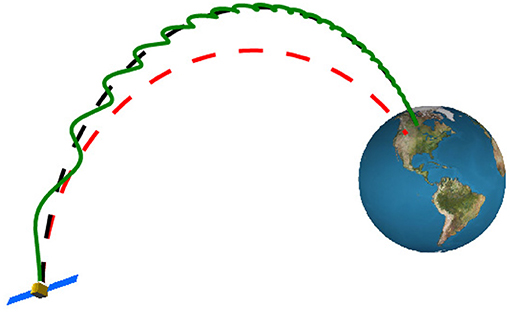
Figure 1. Sketch of part of the proposed diagnostic system for tracing magnetospheric field lines. A change in magnetospheric conditions, and therefore field geometry (black dashed line shifted to the red dashed line), will result in movement of the beam impact location. Electron gyro-orbits of the beam are exaggerated for clarity.

In regards to beam propagation following injection into the magnetosphere and until precipitation in the upper atmosphere, there are three primary questions:

1. Will the injected electrons reach the upper atmosphere?

2. Will the changing magnetospheric conditions influence the impact location of electrons such that this change is detectable by ground stations?

3. Will the beam density profile at impact with the upper atmosphere be sufficiently narrow to produce an emission signature distinguishable from background noise?

With respect to Question 1, the most fundamental consideration is whether the magnetic field line along which a particle is injected will intersect the Earth. For an arbitrary injection location and unknown field geometry, this is difficult to determine a priori. However, close to the Earth (<10R_E, where R_E is the radius of the Earth) the field geometry is close to that of a dipole, and therefore particles launched from near the geomagnetic equator will most likely be attached to field lines which intersect the Earth. A particle injected onto such a field line will experience an increasing magnetic field strength as it approaches the Earth. If the particle has an initially non-zero magnetic moment, then conservation of magnetic moment and energy will result in parallel kinetic energy being converted into perpendicular kinetic energy during this transition. If the increase in field strength is sufficient, then all of the initial energy may be converted to perpendicular energy and the particle is mirrored at a location outside of the Earth's atmosphere, thus precluding precipitation into the atmosphere. In the language of a magnetic mirror, we consider particles which are initialized such that their mirror radius is smaller than the radius of the Earth to be within the loss cone.

A perfectly uniform, non-relativistic beam injected directly along the field line will have zero magnetic moment, and will therefore always precipitate. A realistic beam, however, always has a finite perpendicular energy spread, known as beam emittance within the literature (see section 2.3 for a formal definition), thus particles will have a non-zero magnetic moment. For relativistic electrons, it is important to consider higher order components of the magnetic moment asymptotic expansion when determining the mirror point. Porazik et al. (2014) shows that the loss cone of viable injection angles narrows for increasing beam energy. Furthermore, for injection from the equatorial plane within the magnetotail, the loss cone is narrowed with increased dipole stretching (and therefore local curvature). In such a geometry it becomes favorable to inject above the equatorial plane where field lines have reduced curvature (Willard et al., 2019). These findings set limitations on the beam energy, injection location, pointing precision and beam emittance for a viable diagnostic system.

This paper seeks to provide insight into Questions 2 & 3 via numerical and analytic analysis of electron beam propagation. The following section discusses the methodology of our analysis and numerical tools. Sections 3, 4 present results which pertain to Questions 2 and 3, respectively. For further details and a more complete picture of this proposed diagnostic, see Sanchez et al. (in preparation).

2. Methodology

2.1. Coordinate Systems

Due to the vastly different length scales and the symmetries of a beam and the magnetosphere, it is necessary to depend on four different coordinate systems. Figure 2 shows how each of these systems are interrelated. The first is a Cartesian coordinate system with basis vectors $\left\{\widehat{\text{X}},\widehat{\text{Y}},\widehat{\text{Z}}\right\}$ and origin at the center of the Earth. The $\widehat{\text{X}}$ direction points from the center of the Earth toward the center of the Sun. The $\widehat{\text{Z}}$ direction points along geomagnetic North, and $\widehat{\text{Y}}=\widehat{\text{Z}}\times \widehat{\text{X}}$. This is generally referred to as the solar magnetic or centered dipole coordinate system.

FIGURE 2

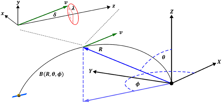
Figure 2. Schematic of the four coordinate systems used within this paper, Earth-centered Cartesian and spherical coordinates, $\left\{\widehat{\text{X}},\widehat{\text{Y}},\widehat{\text{Z}}\right\}$, $\left\{\widehat{\text{R}},\widehat{\theta },\widehat{\varphi }\right\}$ and beam centered Cartesian and spherical coordinates $\left\{\widehat{\text{x}},\widehat{\text{y}},\widehat{\text{z}}\right\}$, $\{\widehat{\text{v}},\widehat{\delta },\widehat{\lambda }\}$.

The second coordinate system is spherical with basis vectors $\left\{\widehat{\text{R}},\widehat{\theta },\widehat{\varphi }\right\}$ and origin collocated with that of the $\left\{\widehat{\text{X}},\widehat{\text{Y}},\widehat{\text{Z}}\right\}$ system. $\widehat{\text{R}}$ points in the radial direction, $\widehat{\theta }$ is the polar angle, measured from the $\widehat{\text{Z}}$ axis and $\widehat{\varphi }$ is the azimuthal angle measured from the $\widehat{\text{X}}$ axis. At the Earth's surface, the angles 90° − θ° and ϕ° correspond to angles of latitude and longitude, respectively, in geomagnetic coordinates.

The third coordinate system is Cartesian with basis vectors $\left\{\widehat{\text{x}},\widehat{\text{y}},\widehat{\text{z}}\right\}$ and origin at the location of a moving test particle, or average location of a collection of particles which make up a beam. The $\widehat{\text{z}}$ vector points along the local magnetic field line, the $\widehat{\text{x}}$ vector is normal to $\widehat{\text{z}}$ and lies along the $\widehat{\text{X}}\times \widehat{\text{Y}}$ plane, and $\widehat{\text{y}}=\widehat{\text{z}}\times \widehat{\text{x}}$.

The fourth coordinate system is spherical with basis vectors $\left\{\widehat{\text{v}},\widehat{\delta },\widehat{\lambda }\right\}$ and describes the particle velocity vector with respect to the local magnetic field. The origin of the system is collocated with the $\left\{\widehat{\text{x}},\widehat{\text{y}},\widehat{\text{z}}\right\}$ system. $\widehat{\delta }$ is the polar angle measured from the $\widehat{\text{z}}$ axis and $\widehat{\lambda }$ is the azimuthal angle measured with respect to the $-\widehat{\text{y}}$ direction.

2.2. Magnetic Field Geometry

For much of this theoretical analysis, a simple dipole model for the Earth's magnetosphere is used, centered in the Cartesian or spherical Earth-based coordinate systems and with dipole moment D pointing along the $-\widehat{\text{Z}}$ axis. This field has magnetic vector potential,

$\begin{array}{ll}\text{A}=-\frac{D}{R^2}sin\theta \widehat{\text{Z}}& (1)\end{array}$

where, for a best fit with the Earth's magnetosphere D = |D| = 8.60 × 10¹⁵ T·m³ (Porazik et al., 2014). This yields magnetic field components and magnitude,

$\begin{array}{ll}\text{B}=\nabla \times \text{A}=-\frac{D}{R^3}\left(2cos\theta \widehat{\text{X}}+sin\theta \widehat{\text{Y}}\right)& (\mathrm{2a})\end{array}$

$\begin{array}{ll}B=\left|\text{B}\right|=D\frac{\sqrt{4-3{sin}^2\theta }}{R^3},& (\mathrm{2b})\end{array}$

which describe field lines with profile,

$\begin{array}{ll}R=R_0{sin}^2\theta & (3)\end{array}$

where R₀ is the point at which the field line intersects the magnetic equatorial plane (the $\widehat{\text{X}}\times \widehat{\text{Y}}$ plane), also commonly known as L within the literature. The polar angle with which a field line intersects the Earth's surface θ_E can be found by inverting Equation (3) with R = R_E, where R_E = 6, 371 km is the radius of the Earth,

$\begin{array}{ll}{\theta }_E={sin}^{-1}\sqrt{\frac{R_E}{R_0}}& (4)\end{array}$

In addition to this simple model, realistic semi-empirical magnetic field geometry is implemented to study the effect of different magnetospheric conditions on particle trajectories. This geometry is implemented via the BATS-R-US (Powell et al., 1999; Tóth et al., 2012) package, as part of the Space Weather Modeling Framework (Tóth et al., 2005). The package solves for field geometry via the three-dimensional magneto-hydrodynamic equations on an adaptive grid with solar wind input data being supplied by the NASA Advanced Composition Explorer satellite (Stone et al., 1998).

2.3. Beam Parameters

A compact satellite-mounted particle accelerator of the radio-frequency (RF) type produces an electron beam which is non-uniform along the direction of propagation. The beam consists of periodic structures with various time and length scales (see Figure 3). The smallest scale structures are so called “micro-pulses” which are synchronized with the RF cycle. Multiple micro-pulses form a “mini-pulse,” a collection of which then forms one “pulse.” The timing of each mini-pulse, pulse and the subsequent entire “burst” of each beam firing is determined by the physics of the particle accelerator, spacecraft power limitations and scientific goals of the mission.

FIGURE 3

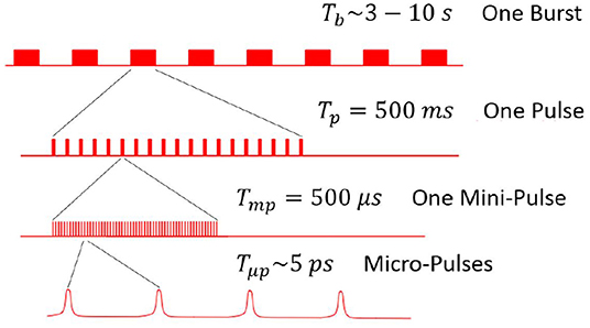
Figure 3. Periodic structures and their respective typical time scales of relativistic electrons produced by a compact radio-frequency particle accelerator.

In this paper we consider down to the time scale of a mini-pulse since for typical energy spreads of RF accelerators the micro-pulse structure will quickly become indistinguishable over the path lengths considered. The largest time scale considered is that of a single pulse, since mission requirements demand that a single pulse impacting the atmosphere be detectable by ground stations.

The electron beam reference conditions of Table 1 are used throughout much of this work.

TABLE 1

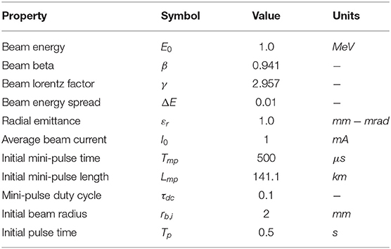
Table 1. Physical parameters of the reference relativistic electron beam.

Based on these properties, the initial phase space profile of a mini-pulse aligned with the local magnetic field vector is given by,

$\begin{array}{l}f(x,y,z,v_x,v_y,v_z,t=0)=f_{0}exp\left(-\frac{x^2+y^2}{2r_{b,i}^2}-\frac{z^2}{2{(L_{mp}/2)}^2}\right)\\ exp\left(-\frac{v_x^2+v_y^2}{2{\langle v_{\perp }\rangle }^2}-\frac{{(v_z-v_0)}^2}{2{\langle v_{\parallel }\rangle }^2}\right),& (5)\end{array}$

where v₀ = βc, $\langle v_{\parallel }\rangle =q_e{E}_0\Delta E/m_{e}c\beta {\gamma }^3$ is the RMS longitudinal velocity spread, and 〈v_⊥〉 = ε_rv₀/r_{b, i} is the RMS radial velocity spread. Here ε_r is the beam emittance (note that the symbol ε_r is used to distinguish it from the small parameter ϵ used throughout this text). For a beam not initially aligned with the local field, the profile of Equation (5) will be tilted via angles δ and λ as per Figure 2.

2.4. Numerical Methods

For the numerical aspect of this work, simulations were performed with a single-particle-motion, ballistic propagation code, first used and verified in Porazik et al. (2014). The code initializes one beam pulse, consisting of a fixed number of mini-pulses. Each mini-pulse consists of a statistical distribution of particles spread in six-dimensional phase space (see Equation 5) and initialized via a pseudo-random number generator. The particles are evolved via the standard Boris algorithm (Boris, 1970) from some injection location (X, Y, Z) with provided injection angle (δ, λ), along a prescribed magnetic field, until each particle has impacted the Earth (R < R_E) or the simulation time ends.

The code can incorporate either an analytic magnetic dipole field or take BATS-R-US data as an input. In the case of BATS-R-US data, magnetic field line information is interpolated to the particle location via a three-dimensional spline interpolation tool.

A limitation of the ballistic code is that it does not capture self-consistent collective interactions between the electron beam and itself, or the ambient plasma. In section 4.4, we demonstrate that for beam properties near those of the reference conditions (see Table 1), the interaction of the beam with itself plays a small role compared to the independent motion of each particle. Interaction between the beam and the ambient plasma, however, may result in instabilities which act to spread the beam. Simple linear analysis suggests that a beam propagating through the magnetosphere will be stable to two-stream instabilities (Galvez and Borovsky, 1988), resistive hose, ion hose and filamentation instabilities (Gilchrist et al., 2001). A more detailed non-linear analysis is required and will be reserved for a future publication.

3. Beam Impact Location

In this section we consider the second question posed in the introduction to this paper, whether changing magnetospheric conditions will influence the impact location of the beam such that this change will be detectable by ground stations.

The section begins by studying the motion of a single electron with energy E₀ injected onto a dipole field line until it impacts with the Earth. We show that it is reasonable to assume conservation of the magnetic moment, an important result for the theoretical results of this paper. We then measure the offset of the final impact location with respect to the original field line due to particle drifts and compare this to analytic theory. Realistic magnetic field geometry is then considered, demonstrating that changes in magnetospheric conditions will appreciably shift the beam impact location.

3.1. Effect of Single-Particle-Motion Drifts

A single electron is injected from $-10R_E\widehat{\text{X}}$ with energy E₀ = 1 MeV from Table 1 and an initial velocity vector along the local dipole field line (in the $\widehat{\text{Z}}$ direction). The initial field line and trajectory of the electron from injection until impact with the Earth is shown on the three Cartesian planes in Figure 4 (note the exaggerated scale in the Y-direction). Total time of flight is t_f = 289 ms and the particle impacts 6.2 km east of the field line intersection point with the Earth.

FIGURE 4

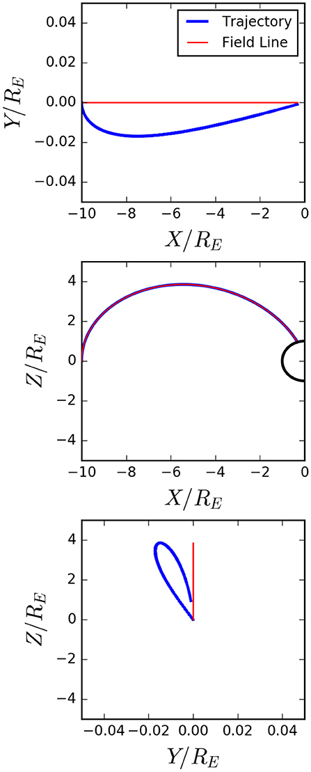
Figure 4. Trajectory of a single electron (blue) injected from $-10R_E\widehat{\text{X}}$ along a dipole field line (red).

If the distance traveled by the particle during one cyclotron orbit L_c is small in comparison to the gradient length scale of the magnetic field L_B, then we can assume that the magnetic moment μ is conserved to all orders. This ratio is largest during particle injection, when the ambient field strength is weakest. From Equation (2b), this ratio is computed as,

$\begin{array}{ll}\begin{array}{c}ϵ=\frac{L_c}{L_B}=\frac{v_0}{{\omega }_c}/\left|\frac{B}{dB/dR}\right|=\frac{3m_0\gamma \beta c{R}_0^2}{qD}\end{array}& (6)\end{array}$

where m₀ is the rest mass of the electron and q is the fundamental charge.

For these injection conditions, we have ϵ ≈ 6.7 × 10⁻³ and can therefore safely assume conservation of μ. Departure of the particle trajectory from the magnetic field line in the $-\widehat{\text{Y}}$ direction can therefore be accurately described by single-particle-motion drifts. The particle initially drifts away from the field line and then appears to return due to the radial convergence of the field lines approaching the Earth. For a relativistic electron, the drift velocity due to curvature and ∇B drifts is given by,

$\begin{array}{ll}{\text{v}}_d=\frac{\gamma m_0}{2q}\left(2v_{\parallel }^2+v_{\perp }^2\right)\frac{\text{B}\times \nabla B}{B^3}& (7)\end{array}$

where v_∥ = v₀ cos δ and v_⊥ = v₀ sin δ are the parallel and perpendicular velocity components, respectively, and with reference to the local magnetic field.

Assuming that v_⊥ ≪ v_∥ ≈ v₀, using the field line geometry from Equation (2b) and integrating over the field line path, the total displacement of the particle impact location from the field line intersection point can be approximated as,

$\begin{array}{ll}\Delta D\approx 1.131\frac{m_0\gamma \beta c{R}_E^3}{qD}{\left(\frac{R_0}{R_E}\right)}^{3/2}& (8)\end{array}$

For our reference beam conditions ΔD ≈ 5.9 km, which is in reasonable agreement with the simulation.

3.2. Change in Impact Location With Magnetospheric Conditions

To explore the influence of magnetospheric conditions on the impact location of the beam, we simulate the injection of an electron into realistic BATS-R-US magnetospheric field geometry. The test case is the St. Patrick's day magnetospheric storm over the 17th and 18th of March 2015 (Jacobsen and Andalsvik, 2016). Simulations were run for seven different magnetospheric conditions, encompassing the pre-storm, Interplanetary Shock (IPS) arrival, storm main and recovery phases. Particles are injected from the equatorial plane at $-5R_E\widehat{\text{X}}$ on the midnight side of the noon-midnight meridian. Injection from this distance results in a favorable probability of injection into the loss-cone (see Willard et al., 2019 for further details).

Figure 5 shows the trajectory of each electron, which closely match that of their respective field lines. The final impact locations of each pulse are converted from geomagnetic coordinates to true longitude and latitude coordinates via the International Geomagnetic Reference Field (Thébault et al., 2015). The impact longitude is then shifted by some reference value to indicate impact over the North American continent, Figure 6 shows the impact location of each of the beams. The separation of the impact positions clearly demonstrates that different phases of the storm will be highly distinguishable due to several-degree latitude separation between impact locations. Results from section 4 will show that these shifts are many orders of magnitude larger than the beam spot size at the top of the atmosphere and therefore will be clearly separable in ground station measurements. It is important to point out that ground stations will clearly need to be placed to cover observation over very large areas, particularly during intense geomagnetic activity when impact locations can be separated by more than 2,000 km.

FIGURE 5

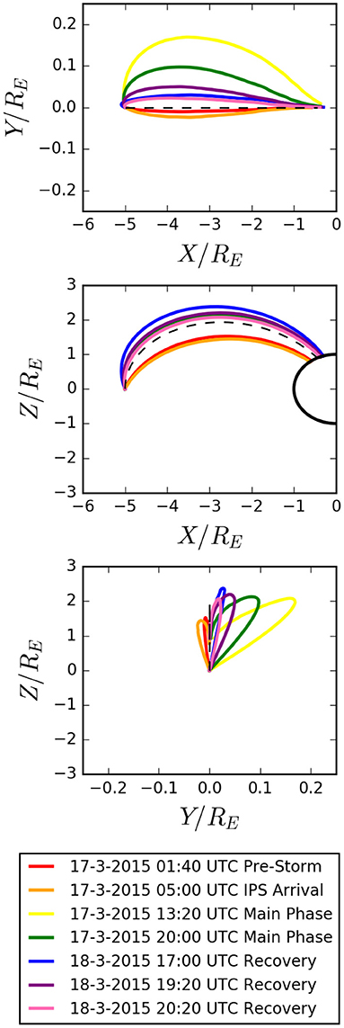
Figure 5. Trajectories of beam particles emitted from $-5R_E\widehat{\text{X}}$ during various phases of the 2015 St. Patrick's Day magnetospheric storm.

FIGURE 6

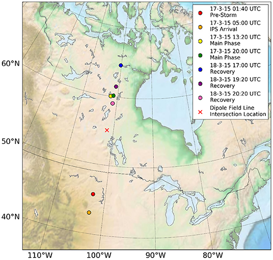
Figure 6. Impact locations of electrons emitted from $-5R_E\widehat{\text{X}}$ during various phases of the 2015 St. Patrick's Day magnetospheric storm. Impact locations vary by hundreds or thousands of kilometers depending on the storm phase.

In this idealized hypothetical diagnostic campaign, it is assumed that the satellite will be capable of injecting particles from an identical location at all times. Although this scenario provides clarity regarding Question 2, as posed in the introduction, it will most likely not be the case in reality. While a more thorough investigation of orbits is ongoing, possible realistic orbits could include geosynchronous, or sun-synchronous orbits, with perigee and apogee ranging between 5−10R_E, allowing for multiple injection radii to be sampled.

4. Evolution of Beam Cross-Section Density Profile

In this section we consider the third question posed in the introduction to this paper, whether the beam will remain sufficiently focused during propagation. This can be determined by studying the evolution of the beam cross-section density profile from injection to impact with the Earth. The evolution of the beam density profile will be affected by beam initial conditions; energy, energy spread, emittance, beam radius and injection angles, as well as the geometry of the magnetospheric field lines.

Significant headway can be made in this analysis by considering a simple ensemble of electrons moving in a uniform magnetic field. Let the electrons evolve in the $\widehat{\text{x}}\times \widehat{\text{y}}$ plane with magnetic field in the $\widehat{\text{z}}$ direction. Each particle has initial velocity vector ${\text{v}}_{\perp }(t=0)=(v_{\perp }+\delta v_x)\widehat{\text{x}}+\delta v_y\widehat{\text{y}}+v_{\parallel }\widehat{\text{z}}$ with δv_x and δv_y randomly sampled from a two-dimensional Maxwellian distribution with RMS velocity 〈v_⊥〉 given by the beam emittance ε_r. From Newton's second law and the Lorentz force law, particle positions will evolve as,

$\begin{array}{ll}\begin{array}{c}x(t)=\frac{v_{\perp }}{{\omega }_c}sin({\omega }_{c}t)+\frac{\delta v_x}{{\omega }_c}sin({\omega }_{c}t)-\frac{\delta v_y}{{\omega }_c}cos({\omega }_{c}t)\\ y(t)=\frac{v_{\perp }}{{\omega }_c}cos({\omega }_{c}t)+\frac{\delta v_x}{{\omega }_c}cos({\omega }_{c}t)+\frac{\delta v_y}{{\omega }_c}sin({\omega }_{c}t)\end{array}& (9)\end{array}$

where ω_c = qB/γm₀ is the relativistic electron cyclotron frequency.

The first component of each equation describes simple cyclotron motion with radius r_c = v_⊥/ω_c. The remaining two components of each equation describe the evolution of the beam RMS radius r_b, also known as the beam envelope,

$\begin{array}{ll}{r}_b=\sqrt{{\langle \delta v_x\rangle }^2+{\langle \delta v_y\rangle }^2}=\frac{\langle v_{\perp }\rangle }{{\omega }_c}(1-cos({\omega }_{c}t))& (10)\end{array}$

The envelope of the ensemble of particles is therefore expanding and contracting on the cyclotron time scale and in phase with the centroid motion of the entire beam rotating at radius r_c. In sections 4.1 and 4.4 below, we show that for conditions near the reference values we generally have r_c>r_b, and therefore, shortly after injection the beam density profile evolves similar to that shown in Figure 7A.

FIGURE 7

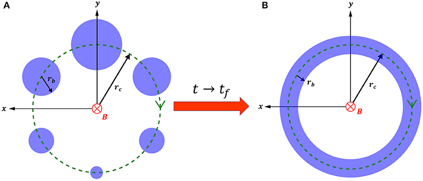
Figure 7. Schematic of the beam cross-section density profile evolution, view from behind the beam looking along the field line. The beam centroid motion and envelope expansion and contraction are decoupled, but in phase, resulting in a cross section profile similar to that in (A). As the beam approaches Earth, the spread in gyro-frequency evolves this profile into that of corkscrew, which is projected onto the atmosphere as a ring in (B).

Since there is a spread in beam energy the cyclotron frequencies of each particle will differ slightly due to the Lorentz factor γ in the denominator. The RMS spread in the cyclotron frequency ω_c is approximately related to the energy spread via,

$\begin{array}{ll}\Delta {\omega }_c\approx \frac{q^{2}B{E}_0}{{(\gamma mc)}^2}\Delta E& (11)\end{array}$

In section 4.3, we show that for near beam reference conditions, and injection from 10R_E, the particles will spread many periods in gyro-phase during their time of flight and that the beam density profile will evolve into that of a corkscrew as their gyro-phase and position along the beam are spread. At impact with the atmosphere, this corkscrew will be projected into a ring, as shown in Figure 7B.

In the following sections, the relative magnitudes of the centroid cyclotron radius r_c and beam envelope radius r_b are computed via a more complete analysis. This analysis includes the effects of finite mini-pulse size, finite pulse length, emittance, energy spread, beam self-forces and magnetic field geometry. Without loss of generality, we can continue to decouple the evolution of the beam centroid motion from that of the beam envelope (Qin et al., 2010, 2011; Chung and Qin, 2018). We thus proceed by considering the evolution of the beam centroid and the gyro-phase spread due to energy spread. We then study the evolution of the beam envelope and show that the final envelope size is generally smaller than the beam cyclotron radius. Next, we consider the optimum injection angle for a beam and derive restrictions on the pointing accuracy of the satellite, as well as the loss fraction of particles for beams with large emittance. Finally, we incorporate the motion of the satellite into our calculations and compare these results to ballistic simulations.

4.1. Evolution of Beam Mini-Pulse Centroid

Evolution of the beam centroid is modeled by the dynamics of a single electron injected into an ideal dipole magnetosphere. It is assumed that the electron has properties near to those of the beam reference conditions. Since the particle is relativistic, higher order terms of the asymptotic expansion must be considered when computing the magnetic moment (Porazik et al., 2014). For an axisymmetric field and a particle injected from the geomagnetic mid-plane, a second order expression for the magnetic moment at injection is given by (Gardner, 1966),

$\begin{array}{ll}\mu \approx {\mu }^{(0)}+{\mu }^{(1)}+{\mu }^{(2)}& (\mathrm{12a})\end{array}$

$\begin{array}{ll}{\mu }^{(0)}=\frac{m{v}_{\perp }^2}{2B}& (\mathrm{12b})\end{array}$

$\begin{array}{ll}{\mu }^{(1)}=-\frac{m^2{B}^{\prime }}{2q{B}^3}\left(v_0^2+v_{\parallel }^2\right)v_{\lambda }& (\mathrm{12c})\end{array}$

$\begin{array}{l}{\mu }^{(2)}=\frac{m^3}{2q^2}\{\frac{B^{\prime }{}^2}{B^5}\left[\frac{1}{2}\right(3v_{\lambda }^2+v_{\parallel }^2\left)\right(v_0^2+v_{\parallel }^2)+\frac{3}{8}{v}_{\perp }^4]\\ -\frac{B^{″}}{2B^4}[v_{\lambda }^2{v}_{\parallel }^2+(v_{\lambda }^2+\frac{1}{4}{v}_{\perp }^2\left)\right(v_0^2+v_{\parallel }^2\left)\right]\\ +\frac{B^{\prime }}{2r{B}^4}[v_{\lambda }^2{v}^2-v_{\perp }^2{v}_{\parallel }^2-\frac{5}{4}{v}_{\perp }^2(v_0^2+v_{\parallel }^2)+2v_{\lambda }^2{v}_{\parallel }^2]\}& (\mathrm{12d})\end{array}$

Where v_⊥ = v₀sinδ, v_λ = v_⊥ sin λ, v_∥ = v₀ cos δ and B′ = dB/dR, and angles δ and λ are illustrated in Figure 2. In a dipole field, and when δ ≪ 1, such that v_λ ≤ v_⊥ ≪ v_∥ ≈ v₀, Equation (12) can be approximated as,

$\begin{array}{ll}\mu \approx \frac{m_0\gamma v_{\perp }^2{R}_0^3}{2D}\left(1-2ϵ\frac{v_0}{v_{\perp }}sin\lambda +{ϵ}^2\frac{v_0^2}{v_{\perp }^2}\right)& (13)\end{array}$

Where ϵ is defined in Equation (6). Note that μ ≠ 0 when the particle is injected directly along the field line. With non-zero magnetic moment, the particle will experience magnetic mirroring forces, and therefore a transition from parallel to perpendicular kinetic energy as it moves into an increasing magnetic field strength closer to the Earth. Consider again the example simulation of section 3.1, for a particle injected directly along the field line (δ = 0°) from $-10R_E\widehat{\text{X}}$ and with reference beam properties, at impact 5.7% of the initially parallel kinetic energy is converted into perpendicular kinetic energy, resulting in a cyclotron radius of r_c = 21.8 m.

Although not discussed in detail here, it should be noted that for a particle injected from this location with sufficiently high energy E₀ ⪸ 4 MeV, the particle loss cone may no longer include injection directly along the field line (Porazik et al., 2014).

At impact with the Earth, the magnetic field is strong enough and the perpendicular velocity large enough, that the most significant contribution to the magnetic moment is given by the zeroth order component. Relating the initial magnetic moment, to the final moment at the Earth, ${\mu }_E^{(0)}=\mu$ gives a general relationship for the final cyclotron radius at impact for any particle injected from the geomagnetic equatorial plane onto a dipole field line,

$\begin{array}{ll}{r}_c=\sqrt{\frac{m_0^2{\gamma }^2{\beta }^2{c}^2{R}_E^3}{q^{2}D{B}_E}({sin}^2\delta -2ϵsin\delta sin\lambda +{ϵ}^2)}& (14)\end{array}$

where B_E = B(R_E, θ_E) is the magnetic field strength at the field line intersection point with the Earth.

For δ = 0°, injection from $-10R_E\widehat{\text{X}}$ and reference beam properties, Equation (14) predicts a final cyclotron radius of 21.7 m in near identical agreement to simulations. Figure 8 shows how the final cyclotron radius of this simulation is predicted to vary with injection radius, injection energy and injection angles δ (with fixed λ = −90°), and λ (with fixed δ = 0.5°). These results are verified via ballistic simulations.

FIGURE 8

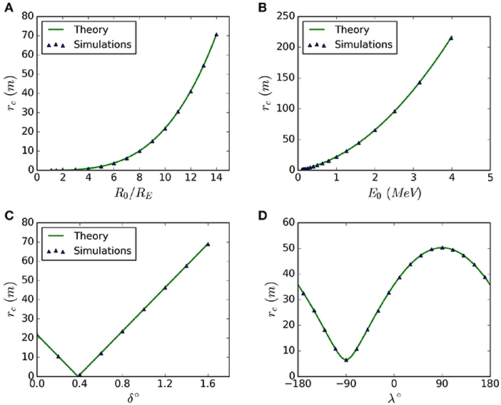
Figure 8. Variation of beam cyclotron radius r_c at impact with the Earth for the reference case (δ = 0°, injection from $-10R_E\widehat{\text{X}}$ and reference beam properties of Table 1) with changes in (A) initial injection radius R₀, (B) initial injection energy E₀, (C) with polar injection angle δ for fixed λ = −90°, (D) with azimuthal injection angle λ for fixed δ = 0.5°.

4.2. Optimum Injection Angle and Pointing Accuracy

Figures 8C,D suggest that there is an optimum injection angle which will minimize the magnetic moment, and therefore final beam centroid cyclotron radius. Figure 8D and Porazik et al. (2014) indicate that the optimum azimuthal injection angle is λ = −π/2. The optimum polar injection angle can be obtained by setting Equation (14) equal to zero, which for small angles gives solution δ ≈ ϵ. Therefore (λ, δ) = (−π/2, ϵ) describe a pair of injection angles which yield zero cyclotron radius at impact with the upper atmosphere.

The limits of the loss cone in a dipole field with λ = −π/2 can be described by Porazik et al. (2014),

$\begin{array}{l}{\text{sin}}^2\delta -\frac{ϵ}{4}\left(5\text{ sin }\delta +\text{ sin }3\delta \right)+\frac{{ϵ}^2}{384}(275+68\text{ cos }2\delta +41\text{ cos }4\delta \\ +4\left(43+\text{ cos }2\delta \right){\text{ sin}}^2\delta )=\frac{{\left(R_E/R_0\right)}^3}{\sqrt{4-3\left(R_E/R_0\right)}}& (15)\end{array}$

Using the small angle approximation, and making the substitution δ → δ_i − ϵ we obtain,

$\begin{array}{ll}{\delta }_i^2\approx \frac{{(R_E/R_0)}^3}{\sqrt{4-3(R_E/R_0)}}& (16)\end{array}$

Where δ_i is the injection angle with respect to the frame shifted by angles (−π/2, ϵ) from the local magnetic field vector. In this frame we recover the traditional circular loss cone, with angular radius defined by δ_i from Equation (16). We can consider δ_i as a minimum bound for the pointing accuracy of the satellite mounted electron accelerator. For standard beam conditions ϵ = 0.38° and ${\delta }_i\approx 1.31^{°}$.

The limits on injection angle may also set restrictions for the radial beam emittance ε_r, which determines the initial radial velocity spread at beam injection. For a sufficiently large ε_r, a significant portion of the injected particles may be injected outside of the loss cone, reducing the signal observed at the top of the atmosphere. For the standard beam conditions, however, we have an RMS spread in injection angles described by $\Delta \delta \approx {\epsilon }_r/r_{b,i}=0.03^{°}$, therefore if fired along the optimum injection angle beam particles will remain well inside the loss cone.

4.3. Spreading of Particle Gyro-Phase Due to Energy Spread

As the particles stream along field lines their gyro-orbits will decorrelate due to a spread in their Lorentz factors γ, and therefore gyro-frequencies. The RMS shift in gyro-phase ψ of a particle with respect to initial energy E₀ can be computed from,

$\begin{array}{ll}\frac{d\psi }{dS}=\frac{\Delta {\omega }_c}{\beta c}=\frac{q^2{E}_0\Delta E}{\beta c^3{\gamma }^2{m}_0^2}B(S)& (17)\end{array}$

Where S is the arc-length of the beam measured from injection and Δω_c is given by Equation (11).

Equation (17) is integrated from injection until impact with the Earth via the ODE integration package LSODE (Hindmarsh, 1980), implemented in Python with SciPy (Oliphant, 2007). The field strength B(S) = B(r(S), θ(S)) is adjusted at each integration point via Equation (2b). For reference beam conditions, Figure 9 shows how the RMS gyro-phase spread changes with time of flight. The rate of phase shift increases closer to the Earth as the particle transits a steeper magnetic field gradient, resulting in a total phase spread of ≈50 gyro-periods. Therefore, the initial centroid motion of the beam mini-pulse will transition into a rotating corkscrew, which projects into a ring at impact with the Earth (see Figure 7).

FIGURE 9

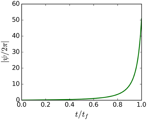
Figure 9. RMS shift in particle gyro orbits against time of flight.

4.4. Evolution of Beam Mini-Pulse Envelope

The beam envelope evolves due to beam initial conditions, self-generated electromagnetic forces, and the applied magnetic field strength. At maximum expansion, the beam mini-pulse length remains ~10³ times longer than the radius, therefore a mini-pulse is modeled as an infinitely long beam. The mini-pulse envelope, r_b evolves according to the one-dimensional beam envelope equation (Reiser, 2008),

$\begin{array}{ll}\frac{d^2{r}_b}{d{S}^2}=-k_0^2{r}_b+\frac{K}{r_b}+\frac{{\epsilon }_r^2}{r_b^3}& (18)\end{array}$

Where $k_0=\frac{qB(S)}{2m_{0}c\gamma \beta }$ is due to focusing from the applied magnetic field and $K=\frac{q{I}_0}{2\pi {\epsilon }_0{m}_0{c}^3{\beta }^3{\gamma }^3}$ is the perveance, which captures the influence of beam self-charge and self-magnetic field, and ε_r is the radial emittance.

Equation (18) is integrated via the same techniques described in section 4.3. Since the ballistic propagation code does not incorporate the effects of space charge, Equation (18) is also solved for the case without perveance (K = 0) to allow for comparison with ballistic simulations.

The solution to the ODE predicts an oscillating beam envelope, however due to gyro-phase mixing the particles will likely fill out a profile at the extrema of these oscillations. The solution to the beam envelope equations with no perveance, and the extrema profiles for the case with and without perveance are shown in Figure 10. Initially the beam radius blows out to a size on the order of hundreds of meters, and then as it propagates toward the Earth, the increasing magnetic field strength focuses the beam. For the reference conditions, the final beam radius at impact with the Earth is 2.6 m with perveance and 2.2 m without perveance.

FIGURE 10

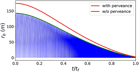
Figure 10. Solution to the envelope equations without beam perveance (blue lines). Extrema solutions with (red) and without perveance (green) for the reference beam conditions.

Equation (18) is solved parametrically to determine the influence on final envelope radius r_{b, f} for changes in initial energy E₀, injection radius R₀, radial emittance ε_r, initial beam radius r_{b, i} and beam current I₀. The results of these parameter scans for cases with and without perveance are shown in Figure 11 along with the corresponding final cyclotron radius r_c for these conditions.

FIGURE 11

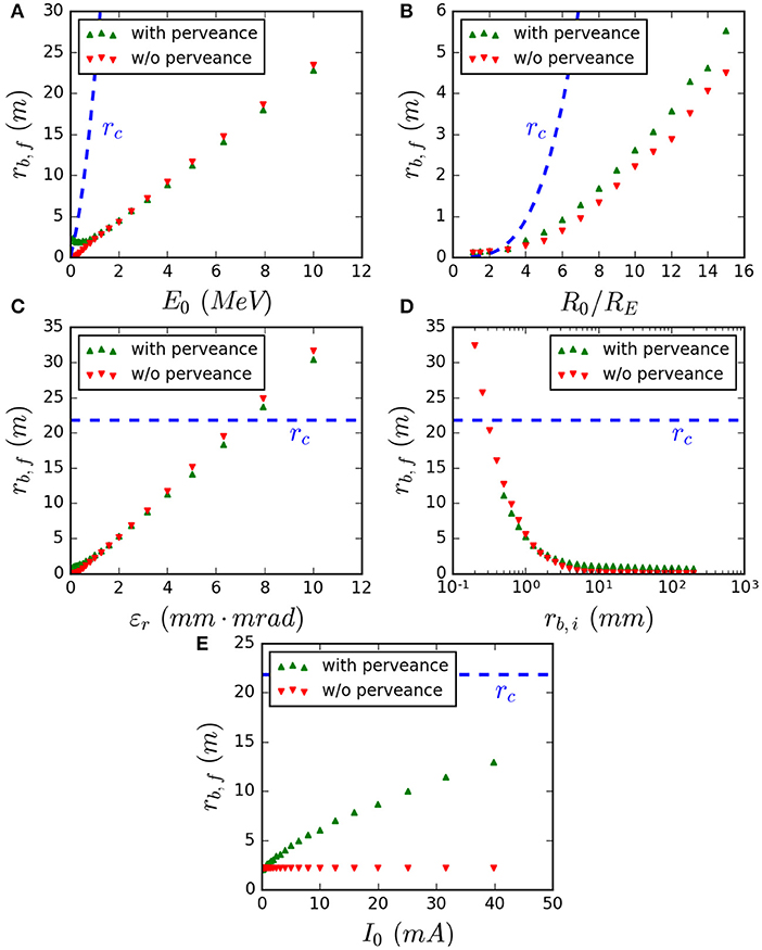
Figure 11. Final RMS beam envelope radius at impact with the Earth with parameter scans in (A) beam energy E₀, (B) injection radii R₀, (C) radial emittance ε_r, (D) initial beam radius r_{b, i}, (E) injection current I₀. Blue dashed lines show the equivalent cyclotron radius for each condition as per Equation (14).

For the reference beam current of 1 mA, the final beam envelope radius is only weakly influenced by beam perveance. This is due to the small magnitude of the average current as well as the self-generated magnetic field which acts to cancel out a large fraction of the beam self-charge for γ ≈ 3. This demonstrates that despite self-forces being neglected, the use of ballistic simulations is suitable for modeling beams with similar properties to those here.

Other observable trends include that increasing the initial beam energy E₀ results in a larger final radii, since the increased electron momentum increases the particle cyclotron radius for the same applied magnetic field. Increasing the beam injection radius R₀ similarly results in an increased final beam radius, due to the weaker magnetic field and therefore larger initial cyclotron radius at injection. Unsurprisingly, increasing beam radial emittance ε_r increases final beam radius since the particles are initialized with a larger RMS perpendicular velocity. Increasing the initial beam radius r_{b, i} results in a smaller final beam radius since the initial current density (and therefore self-electric fields) are reduced. Finally, increasing beam current I₀ results in an increased final radius due to the increased current density at beam initialization. Therefore, the larger the beam current, the less suitable ballistic simulations become for modeling the beam.

It is clear that for conditions near the reference beam properties, the cyclotron radius of the beam centroid dominates the profile of the final particle density distribution since r_{b, f}/r_c ≪ 1. The cyclotron radius r_c is therefore the most important quantity when considering final beam spot size. Figure 11 shows that for increasing beam energy E₀ and injection radius R₀, this ratio will become even smaller. Only for large increases to ε_r, I₀ or decreases to r_{b, i} will this ratio be larger than unity, and then the evolution of the beam envelop may become a more important consideration.

4.5. Effects of Satellite Motion on Beam Pulse Impact Distribution

A single electron beam pulse (see Figure 3) consists of 100 mini-pulses and total pulse time of T_p = 0.5 s. At these time scales it becomes important to consider the motion of the electron gun platform. If this platform were to remain stationary during firing, then the impact density distribution would appear similar to that of a single mini-pulse; however, since the accelerator is attached to a moving satellite, the beam impact location will be smeared out, as each mini-pulse is injected onto a slightly different field line.

Assuming that the satellite is in a circular equatorial orbit, a simple approximation for the satellite angular velocity Ω₀ can be obtained using Newton's second law and equating the gravitational force of the Earth and the centripetal force exerted by the orbiting satellite,

$\begin{array}{ll}{\Omega }_0=\frac{V_0}{R_0}=\sqrt{\frac{G{M}_E}{R_0^3}},& (19)\end{array}$

where G is Newton's gravitational constant and M_E is the mass of the Earth. An equatorial orbit will likely be prograde therefore when calculating the beam impact spread on the surface of the Earth we can subtract the angular velocity of the Earth itself; Ω_E = 2π/T_E, where T_E = 86, 400 s is the period of the Earth's rotation. Therefore the azimuthal shift of the pulse impact location is simply Δϕ = (Ω₀−Ω_E)T_p. Since the dipole field is cylindrically symmetric, the beam spread must be calculated using the cylindrical radius R_Esinθ_E at the impact location of the dipole field line with the Earth. Therefore, the total shift in impact location Δd is given by,

$\begin{array}{ll}\Delta d=R_E\Delta \varphi sin{\theta }_E=T_p{R}_E\left(\frac{\sqrt{G{M}_E{R}_E}}{R_0^2}-\frac{2\pi }{T_E}\sqrt{\frac{R_E}{R_0}}\right)& (20)\end{array}$

Figure 12 shows the pulse impact location displacement against pulse time for various initial injection radii R₀, where Figure 12A shows the case without the Earth's rotation and Figure 12C includes the Earth's rotation. Figures 12B,D show heat maps of the same situation for injection radii under consideration. For the beam reference conditions and injection from 10R_E, the spread of the center of the beam is 79 m.

FIGURE 12

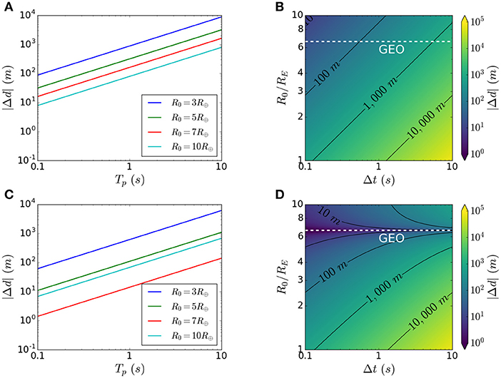
Figure 12. Displacement of the center of the beam spot |Δd| due to motion of a satellite-borne particle accelerator (A,B) satellite motion only, (C,D) satellite motion and Earth rotation. The white dashed line indicates the radius corresponding to Geostationary Orbit (GEO).

4.6. Comparison With Ballistic Simulations

To explore the validity of the above results we simulate a single mini-pulse of electrons injected from 10R_E along a dipole field line. An animation of 200 particles sampled from this simulation can be found here https://youtu.be/ZupUFiF2_yE, and Figure 13A shows the normalized density distribution of particles impacting the upper atmosphere (in the $\widehat{\theta }\times \widehat{\varphi }$ plane). As expected, the impact distribution is ring-shaped rather than circular. The dashed white line shows the predicted final cyclotron radius r_c = 21.8 m from Equation (14). Despite decorrelation of particle gyro-orbit phase, the brighter region at the bottom of the ring demonstrates that a large number of the particles remain closely correlated. In reality, the beam perveance will modify the oscillation frequency of the beam envelope, and therefore if beam self-forces were included we would expect a more uniform distribution of density around the ring.

FIGURE 13

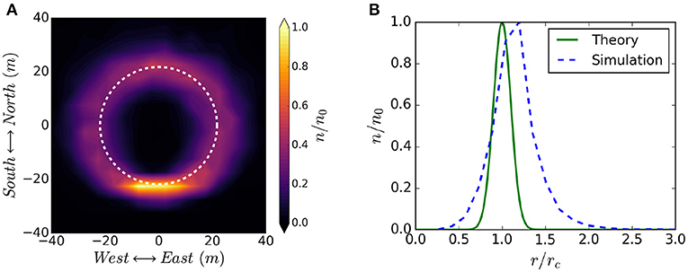
Figure 13. (A) Normalized electron density distribution at impact with the Earth, the theoretically predicted cyclotron radius from Equation (14) is overlayed as a dashed white line. (B) Normalized radial electron density distribution compared with theoretical predictions for beam cyclotron radius (distribution mean) and final beam envelope RMS radius (distribution spread). An animation of beam particle evolution from injection until impact with the atmosphere for these results can be viewed here: https://youtu.be/ZupUFiF2_yE.

Figure 13B shows the radial electron density distribution (measured with respect to the origin in Figure 13A) and the predicted density distribution given by $n/n_0=exp({(r-r_c)}^2/2r_{b,f}^2)$. The mean location of these two profiles show agreement within 15% between the final cyclotron radius of the simulation and the prediction of Equation (14). There is less clear agreement between the simulated and predicted RMS beam envelope radii, with the simulation showing an envelope radius approximately double that of the 2.2 m predicted by solving Equation (18). A possible explanation for this discrepancy is that the energy spread ΔE results in additional beam broadening in the East to West direction due to the energy dependence of the ∇B and curvature drifts. Particles with higher energy will drift further to the East than those with lower energy, resulting in a smearing of the density profile. This may also explain the small discrepancy between the predicted and observed average cyclotron radii.

For completeness we have also produced an animation demonstrating reflection of the beam due to magnetic mirroring. This simulation is for identical conditions, except with injection angles δ = 2°, λ = −90° and can be found here https://youtu.be/Y-amwRDZruo.

Next, 100 mini-pulses, which comprise a single electron pulse, are injected with beam reference properties along a dipole field line from 10R_E. The final normalized impact density distribution is shown in Figure 14. The white dashed line shows the theoretically predicted cyclotron radius combined with the drift predicted due to satellite motion from Equation (20) (without Earth rotation). The center of the spot appears filled out when compared to that of the mini-pulse in Figure 13, and is caused by smearing of the impact ring due to satellite motion. The effect of the true satellite motion and relative rotation of the Earth can be incorporated for specific orbital parameters if required. Details of beam mini-pulse overlapping can be found in the Appendix to this publication.

FIGURE 14

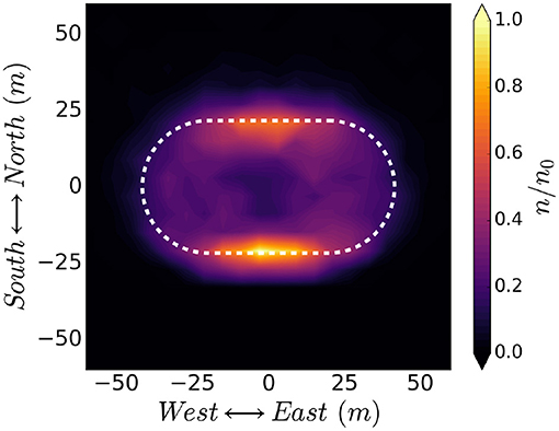
Figure 14. Normalized particle density distribution of a beam pulse at impact with the Earth's atmosphere in the case of a moving satellite, the estimated cyclotron radius and spread due to satellite motion is shown as a dashed white line.

At impact with the atmosphere, relativistic electrons produce very-low frequency (VLF) waves due to secondary ionization, optical emissions due to excitation of neutrals and high energy photons due to bremsstrahlung (Marshall et al., 2014). If their signature is strong enough, both VLF waves and optical spectra can be detected by ground stations, and high energy photons may be observed by high altitude or orbital observatories.

Beam properties at the top of the atmosphere can be used as initial conditions for Monte-Carlo collision models, such as those developed in Marshall et al. (2014), to determine the emission profile of the beam interacting with the atmosphere. Optical emission occurs mostly within the D region of the atmosphere once the beam has spread out to hundreds of meters in radius. The optical photon flux is therefore relatively insensitive to beam radius at the top of the atmosphere, provided r_{b, f} ≲ 100 m, which is satisfied for the reference beam conditions. Specific ground station sensors can then be considered to determine a signal-to-noise ratio, and therefore whether the beam will be detectable.

Marshall et al. (2014) shows that for similar beam energies and fluxes referred to in this paper, the resulting emission spectra will produce significant and detectable signatures. Private communications between users of these tools confirm that this is the case, and further details can be found in Sanchez et al. (in preparation).

5. Conclusion

This paper explores the dynamics of an electron beam propagating from injection into the magnetosphere until impact with the Earth. Injected from the geomagnetic equatorial plane along a dipole field line, particles were found to shift from their original field line due to single-particle-motion drifts. The total integrated drift motion is on the order of kilometers, and therefore when compared to the radius of the Earth the particle impact location is nearly identical to that of the field line intersection point.

Particles were injected from an identical location at 5 Earth radii during different phases of a simulated magnetospheric storm. The phase of the storm was found to strongly influence the impact location of the particles, shifting them hundreds to thousands of kilometers. This simulated diagnostic campaign demonstrates that even for injection radii near to geostationary orbit, magnetospheric weather can have a large observable influence on the impact location of a beam propagating from a satellite down into the atmosphere. It also demonstrates that a wide ground station coverage area will be required to detect these signatures.

Evolution of the beam cross-section was studied by considering the separate dynamics of the beam centroid motion and evolution of the beam envelope. For beam properties near those considered in this work, the final beam centroid cyclotron radius was found to be the most important parameter when estimating the beam spot size at the top of the atmosphere. For the provided beam reference conditions, a single beam mini-pulse impacts with a density profile in the shape of a ring, with major radius ~22 m, and ring thickness ~2 m. When considering a single pulse (multiple mini-pulses) the beam spot size is additionally spread 10 s to 100 s of meters due to motion of the orbiting electron accelerator. With sufficient pointing accuracy and with reference beam emittance, it is possible to inject beam particles into the loss cone. It is shown that the beam spot size will remain sufficiently narrow to allow detection from ground stations on the surface of the earth. Future work will explore how beam-plasma instabilities may modify the final beam spot size.

Demonstrating theoretically that the beam will be detectable by ground stations, and that magnetospheric events will significantly influence the beam impact location provides validation for two of the key requirements of this proposed diagnostic.

Data Availability Statement

The datasets generated for this study are available on request to the corresponding author.

Author Contributions

AP contributed significantly to original research, and prepared the manuscript. PP contributed significantly to original research in this article. MG-M, KA, and DS contributed to original research for this article. IK, JJ, and ES are principal investigators for this research, they contributed and guided this research.

Funding

This research was funded by NSF's INSPIRE initiative through grant 1344303.

Conflict of Interest

The authors declare that the research was conducted in the absence of any commercial or financial relationships that could be construed as a potential conflict of interest.

The handling editor declared a past co-authorship with one of the authors ES.

Acknowledgments

The authors would like to thank their fellow members of the team, with specific thanks to Prof. Robert Marshall and Dr. Eric Dors for their contributions to this work.

This work was carried out using the SWMF/BATSRUS tools developed at The University of Michigan Center for Space Environment Modeling (CSEM) and made available through the NASA Community Coordinated Modeling Center (CCMC).

A great deal of this work would not have been possible without the support of numerous undergraduate students through the Department of Energy's Science Undergraduate Laboratory Internships program, and high school students supported by the Princeton Plasma Physics Laboratory Science Education Program.

Supplementary Material

The Supplementary Material for this article can be found online at: https://www.frontiersin.org/articles/10.3389/fspas.2019.00069/full#supplementary-material

References

Banks, P., Fraser-Smith, A., Gilchrist, B., Harker, K., Storey, L., and Williamson, P. (1987). New Concepts in Ionospheric Modification. Technical report, Stanford Univ CA Space Telecommunications and Radioscience Lab (STAR).

Google Scholar

Boris, J. P. (1970). “Relativistic plasma simulation-optimization of a hybrid code,” in Proceedings of the Fourth Conference Num. Sim. Plasmas, Naval Research Laboratory (Washington, DC), 3–67.

Google Scholar

Chung, M., and Qin, H. (2018). Generalized parametrization methods for centroid and envelope dynamics of charged particle beams in coupled lattices. Phys. Plasmas 25:011605. doi: 10.1063/1.5018426

CrossRef Full Text | Google Scholar

Galvez, M., and Borovsky, J. E. (1988). The electrostatic two-stream instability driven by slab-shaped and cylindrical beams injected into plasmas. Phys. Fluids 31, 857–862. doi: 10.1063/1.866767

CrossRef Full Text | Google Scholar

Gardner, C. (1966). Magnetic moment to second order for axisymmetric static field. Phys. Fluids 9, 1997–2000. doi: 10.1063/1.1761557

CrossRef Full Text | Google Scholar

Gendrin, R. (1974). The french-soviet araksexperiment. Space Sci. Rev. 15, 905–931. doi: 10.1007/BF00241068

CrossRef Full Text | Google Scholar

Gilchrist, B. E., Khazanov, G., Krause, L., and Neubert, T. (2001). Study of Relativistic Electron Beam Propagation in the Atmosphere-Ionosphere-Magnetosphere. Technical report, Michigan University, Ann Arbor, MI.

Google Scholar

Hendrickson, R., McEntire, R., and Winckler, J. (1971). Electron echo experiment: a new magnetospheric probe. Nature 230:564. doi: 10.1038/230564a0

CrossRef Full Text | Google Scholar

Hess, W., Trichel, M., Davis, T., Beggs, W. C., Kraft, G. E., Stassinopoulos, E., et al. (1971). Artificial aurora experiment: experiment and principal results. J. Geophys. Res. 76, 6067–6081. doi: 10.1029/JA076i025p06067

CrossRef Full Text | Google Scholar

Hindmarsh, A. C. (1980). Lsode and lsodi, two new initial value ordinary differential equation solvers. ACM Signum Newslett. 15, 10–11. doi: 10.1145/1218052.1218054

CrossRef Full Text | Google Scholar

Jacobsen, K. S., and Andalsvik, Y. L. (2016). Overview of the 2015 st. patricks day storm and its consequences for rtk and ppp positioning in norway. J. Space Weather Space Climate 6:A9. doi: 10.1051/swsc/2016004

CrossRef Full Text | Google Scholar

Lewellen, J., Buechler, C., Dale, G., Dolgashev, V., Holloway, M., Jongewaard, E., et al. (2018). “Linac design elements for spaceborne accelerators,” in 9th International Particle Accelerator Conference (IPAC'18), Vancouver, BC, Canada, April 29-May 4, 2018 (Geneva: JACOW Publishing), 4291–4293.

Google Scholar

Marshall, R., Nicolls, M., Sanchez, E., Lehtinen, N., and Neilson, J. (2014). Diagnostics of an artificial relativistic electron beam interacting with the atmosphere. J. Geophys. Res. Space Phys. 119, 8560–8577. doi: 10.1002/2014JA020427

CrossRef Full Text | Google Scholar

Mishin, A. V. (2005). “Advances in x-band and s-band linear accelerators for security, ndt, and other applications,” in Proceedings of the Particle Accelerator Conference, 2005. PAC 2005 (IEEE), 240–244.

Google Scholar

National Research Council (2013). Solar and Space Physics: A Science for a Technological Society. Washington, DC: The National Academies Press.

Google Scholar

Neubert, T., and Gilchrist, B. (2004). Relativistic electron beam injection from spacecraft: performance and applications. Adv. Space Res. 34, 2409–2412. doi: 10.1016/j.asr.2003.08.081

CrossRef Full Text | Google Scholar

Neubert, T., and Gilchrist, B. E. (2002). Particle simulations of relativistic electron beam injection from spacecraft. J. Geophys. Res. Phys. 107:1167. doi: 10.1029/2001JA900102

CrossRef Full Text | Google Scholar

Nguyen, D., Buechler, C., Dale, G., Dolgashev, V., Fleming, R., Holloway, M., et al. (2018). “The path to compact, efficient solid-state transistor-driven accelerators,” in 9th International Particle Accelerator Conference (IPAC'18), Vancouver, BC, Canada, April 29-May 4, 2018 (Geneva: JACOW Publishing), 520–523.

Google Scholar

Oliphant, T. E. (2007). Python for scientific computing. Comput. Sci. Eng. 9, 10–20. doi: 10.1109/MCSE.2007.58

CrossRef Full Text | Google Scholar

Porazik, P., Johnson, J. R., Kaganovich, I., and Sanchez, E. (2014). Modification of the loss cone for energetic particles. Geophys. Res. Lett. 41, 8107–8113. doi: 10.1002/2014GL061869

CrossRef Full Text | Google Scholar

Powell, K. G., Roe, P. L., Linde, T. J., Gombosi, T. I., and De Zeeuw, D. L. (1999). A solution-adaptive upwind scheme for ideal magnetohydrodynamics. J. Comput. Phys. 154, 284–309. doi: 10.1006/jcph.1999.6299

CrossRef Full Text | Google Scholar

Qin, H., Davidson, R. C., and Logan, B. G. (2010). Centroid and envelope dynamics of high-intensity charged-particle beams in an external focusing lattice and oscillating wobbler. Phys. Rev. Lett. 104:254801. doi: 10.2172/981703

PubMed Abstract | CrossRef Full Text | Google Scholar

Qin, H., Davidson, R. C., and Logan, B. G. (2011). Centroid and envelope dynamics of charged particle beams in an oscillating wobbler and external focusing lattice for heavy ion fusion applications. Laser Part. Beams 29, 365–372. doi: 10.1017/S0263034611000401

CrossRef Full Text | Google Scholar

Reiser, M. (2008). Theory and Design of Charged Particle Beams. New York, NY: John Wiley & Sons.

Google Scholar

Stone, E. C., Frandsen, A., Mewaldt, R., Christian, E., Margolies, D., Ormes, J., et al. (1998). The advanced composition explorer. Space Sci. Rev. 86, 1–22. doi: 10.1023/A:1005082526237

CrossRef Full Text | Google Scholar

Thébault, E., Finlay, C. C., Beggan, C. D., Alken, P., Aubert, J., Barrois, O., et al. (2015). International geomagnetic reference field: the 12th generation. Earth Plan. Space 67:79.

Google Scholar

Tóth, G., Sokolov, I. V., Gombosi, T. I., Chesney, D. R., Clauer, C. R., De Zeeuw, D. L., et al. (2005). Space Weather Modeling Framework: a new tool for the space science community. J. Geophys. Res. Space Phys. 110:A12226. doi: 10.1029/2005JA011126

CrossRef Full Text | Google Scholar

Tóth, G., van der Holst, B., Sokolov, I. V., Zeeuw, D. L. D., Gombosi, T. I., Fang, F., et al. (2012). Adaptive numerical algorithms in space weather modeling. J. Comput. Phys. 231, 870–903. doi: 10.1016/j.jcp.2011.02.006

CrossRef Full Text | Google Scholar

Willard, J. M., Johnson, J. R., Snelling, J. M., Powis, A. T., Kaganovich, I. D., et al. (2019). Effect of field-line curvature on the ionospheric accessibility of relativistic electron beam experiments. Front. Astron. Space Sci. 6:56. doi: 10.3389/fspas.2019.00056

CrossRef Full Text | Google Scholar

Winckler, J., Malcolm, P., Arnoldy, R., Burke, W., Erickson, K., Ernstmeyer, J., et al. (1989). Echo 7: an electron beam experiment in the magnetosphere. Eos Trans. Am. Geophys. Union 70, 657–668. doi: 10.1029/89EO00194

CrossRef Full Text | Google Scholar

Winckler, J. R. (1980). The application of artificial electron beams to magnetospheric research. Rev. Geophys. 18, 659–682. doi: 10.1029/RG018i003p00659

CrossRef Full Text | Google Scholar

Winckler, J. R. (1982). “The use of artificial electron beams as probes of the distant magnetosphere,” in Artificial Particle Beams in Space Plasma Studies (Boston, MA: Springer), 3–33.

Google Scholar