A Markov Chain Approximation for American Option Pricing in Tempered Stable-GARCH Models

1. Introduction

It is commonly known that the Black-Scholes model does not describe the real behavior of derivatives very well. The model is not consistent with the observed behavior found in asset returns, such as volatility clustering, skewness and fat tails. Many studies have been conducted to modify Black-Scholes model to incorporate these three empirical features of the asset returns. The α-stable distribution proposed by Mandelbrot [1] is an alternative to the normal distribution for modeling asset returns because it allows for skewness and fat tails. While the α-stable distribution has certain desirable properties, it is not suitable in modeling option prices, because it does not have the second moment or even the first moment. In order to obtain a well-defined model for pricing options, the mean, variance, and exponential moments of the return distribution have to be finite. Therefore, there are many modified distributions proposed for financial modeling based on the α-stable distribution. For example, the classical tempered stable (CTS) distribution [2, 3], normal inverse Gaussian (NIG) distribution [4] and its generalization called normal tempered stable (NTS) distribution [5], the modified tempered stable (MTS) distribution [6] and an extension of the CTS distribution named the KR distribution [7]. These distributions, called the tempered stable distributions, not only can incorporate the fat tails and skewness of asset returns, but also have finite moments for all orders. Furthermore, they are all infinitely divisible, i.e., the random variable can be decomposed to a sequence of i.i.d random numbers from the same family. So each of them uniquely corresponds to a Lévy process. Therefore, by replacing the Brownian motion by these Lévy processes, one can extend Black Scholes model to the so called exponential Lévy models. However, these Lévy exponential models are based on the assumptions that the returns are identically and independently distributed (i.i.d). Therefore, they are not able to explain the volatility clustering phenomena.

GARCH model have been developed to model the asset returns under the assumption of a non- Markovian property, more precisely, the assumption of volatility clustering. In Duan [8, 9], Kallsen[10], Heston [11], and Christoffersen [12] theories have been developed for pricing derivatives contracts using GARCH models. Most of researches assume that the innovations of GARCH are normally distributed. Although one can show that the normal GARCH model has heavier tails than Gaussian white noise, i.e., the kurtosis is greater than 3, it is still not able to fully capture the extreme values and skewness of the return process. To overcome the drawback of normal innovation process, Menn and Rachev [13, 14] introduced an enhanced GARCH model with innovations which follow the smoothly truncated stable distribution. Stentoft [15] proposed a GARCH model with NIG distribution for American option pricing. Kim et al. [7] applied the three tempered stable distributions (CTS, MTS, and KR distributions) to model the residual distribution in the GARCH process, and presented the CTS-GARCH model, MTS-GARCH model, and KR-GARCH model. Kim et al. [16] presented the RDTS-GARCH option pricing model. These models can incorporate the three empirical features of the asset returns pretty well. In this paper, we will consider the two most widely used tempered stable distributions to model the residual distribution: classical tempered stable (CTS) and normal tempered stable (NTS).

However, it is difficult to price American options under the GARCH models with tempered stable distributions. It is widely recognized that the existing methods for pricing American options under GARCH are bivariate tree method and least square simulation method presented by Longstaff and Schwartz [17]. Ritchken and Trevor [18], Duan and Simonato [19] have introduced a modified lattice approach and a Markov chain method, respectively. These methods are applied to price American options under the normal-GARCH model. Rachev et al. [20] applied the least square approach to price American options under different TS-GARCH models. However, the least square method might fail to give accurate results when the option is out of the price [21]. Furthermore, increasing the order of the approximating polynomials may not give a good fit to the price when the returns have heavier tails, i.e., more extreme values.

In this paper, we consider the Markov chain approach presented by Duan and Simonato [19] and apply it to the CTS-GARCH and NTS-GARCH models. The idea of the approach is to discretized the stock price and the volatility, and use a Markov chain to approximate the original process. The fixed partition of the state space simplifies the task of option pricing to a sequence of standard matrix operations.

There are two major difficulties in applying this approach to TS-GARCH models. First, the distribution of the residuals changes over time under the original risk neutral argument of Rachev et al. [20]. Thus, we have to recompute the transition matrix each time which makes the Markov chain approach time-consuming. So we apply the minimal entropy method to determine the risk neutral measure. This method provides a large degree of freedom to construct the model in the risk neutral world. By applying this approach we are allowed to use the same transition matrix when computing the option prices. The second difficulty is how to determine the partition conditions of TS GARCH effectively. The skewness and heavy tails of the tempered stable distributions implies that we need a different way to discretize stock price and volatility in order to make the approximating Markov chain convergent.

The numerical examples shows that the option values computed by the Markov chain method converge to the theoretical value. The computation time of the approach is not as expensive as one might expect since the transition probability matrix is highly sparse. It works well for the TS-GARCH option pricing framework. However, the convergence speed of Markov chain method depends on GARCH parameters. For stocks with relatively higher volatilities, the convergence rate becomes slow even for the normal GARCH model, since we have to increase the range of the stock price and volatilities. It is not strange that the convergence speed under the TS-GARCH model would be slower than the normal GARCH. Nevertheless, the TS-GARCH model captures the stylized facts of the market and therefore provides a better fit to the stock price, see Stentoft [15], Kim et al. [7] and Rachev et al. [20]. In the empirical analysis we illustrate how to apply our approach to compute the American option prices in the real world. Calibrated risk neutral parameters and minimal entropy parameters are computed and compared.

The paper is organized as follows: Section 2 contains the introduction to the GARCH model with the tempered stable distributions. Section 3 presents the Markov chain method under the CTS-GARCH, and NTS-GARCH models. The convergence of the Markov chain method is presented in Section 4. In Section 5, we conduct some numerical experiments and empirical analysis to illustrate our approach. The last section contains the concluding remarks.

2. GARCH Model with Tempered Stable Distributed Innovations

In this section we briefly review the GARCH model with tempered stable innovations introduced by Rachev et al. [20]. Furthermore, we apply the minimal entropy approach to determine the equivalent martingale measure.

2.1. Tempered Stable Distributions

First we introduce two most widely-used tempered stable distributions: the CTS distribution and the NTS distribution.

The CTS distribution with parameter α, C, λ₊, λ₋, m is defined by its characteristic function:

$\begin{array}{l}{\varphi }_{CTS}(u;\alpha ,C,{\lambda }_{+},{\lambda }_{-},m)\\ =\exp (ium-iuC\Gamma (1-\alpha )({\lambda }_{+}^{\alpha -1}-{\lambda }_{-}^{\alpha -1})+\\ C\Gamma (-\alpha )({({\lambda }_{+}-iu)}^{\alpha }-{\lambda }_{+}^{\alpha }+{({\lambda }_{-}+iu)}^{\alpha }-{\lambda }_{-}^{\alpha })),\end{array}$

where C, λ₊, λ₋ > 0, α ∈ (0, 2) \ {1} and m ∈ ℝ. We denote X ~ CTS(α, C, λ₊, λ₋, m) if the random variable X follows CTS distribution. The parameters m and C are the location and scale parameters respectively. α is the key parameter related to the heavy tail. And λ₊ and λ₋ control the rate of decay on the positive and negative tails respectively. The distribution is symmetric if λ₊ = λ₋. A Lévy process induced from the CTS distribution is called the classical tempered stable process with parameters (α, C, λ₊, λ₋, m).

The mean and the variance of the CTS distribution are given by

$\begin{array}{lll}\hfill E\left[X\right]& =m;& \end{array}$

$\begin{array}{lll}\hfill Var(X)& =C\Gamma (2-\alpha )({\lambda }_{+}^{\alpha -2}-{\lambda }_{-}^{\alpha -2}).& \end{array}$

Therefore, if we set m = 0 and

$C=(\Gamma (2-\alpha )({\lambda }_{+}^{\alpha -2}-{\lambda }_{-}^{\alpha -2})){}^{-1},$

then X has zero mean and unit variance. In this case, we say that X follows the standard CTS distribution with parameters (α, λ₊, λ₋) and denoted by X ~ stdCTS(α, λ₊, λ₋).

Let α ∈ (0, 2), θ, γ > 0 and β, m ∈ ℝ. X is said to follow the normal tempered stable (NTS) distribution, if the characteristic function of X is given by:

$\begin{array}{l}{\varphi }_{NTS}(u;\alpha ,\theta ,\gamma ,\beta ,m)\\ =\exp \left(iu(m-\beta )-\frac{2{\theta }^{1-\frac{\alpha }{2}}}{\alpha }\left({\left(\theta -i\beta u+\frac{{\gamma }^2{u}^2}{2}\right)}^{\frac{\alpha }{2}}-{\theta }^{\frac{\alpha }{2}}\right)\right).\end{array}$

We denote an NTS distributed random variable X by X ~ NTS(α, θ, γ, β, m). α and θ control the rate of tail decay; γ and β control the variance; and β determines the skewness. If β > 0, the distribution is skewed to the left. The mean and variance of NTS are given by

$\begin{array}{lll}\hfill E\left[X\right]& =m;& \end{array}$

$Var(X)={\gamma }^2+{\beta }^2\left(\frac{2-\alpha }{2\theta }\right).$

If $|\beta |<\sqrt{\frac{2\theta }{2-\alpha }}$, then we are able to set m = 0 and $\gamma =\sqrt{1-{\beta }^2(\frac{2-\alpha }{2\theta })}$ so that X has zero mean and unit variance. In this case, we say that X follows the standard NTS distribution and denoted by X ~ stdNTS(α, θ, β).

The tempered stable distributions, including CTS and NTS, have heavier tails than Gaussian distribution. On the other hand, their tails are thinner than the α-stable distribution whose tail has a power decay. One can show that the moments of CTS and NTS are all finite. For details we refer to Cont and Tankov [22] and Rachev et al. [20].

2.2. GARCH Option Pricing Model

2.2.1. Under the Market Measure ℙ

In this section we introduce the GARCH model with heavy tailed distributions under the market measure. We do not consider dividends here for simplicity. Let (Ω, {${F}$_t}_{t = 0, 1, …, T}, ℙ) denote the standard probability space, where ${F}$_t is the sigma algebra represents the information up to time t. We assume that the dynamics of the stock price is given by

$\begin{array}{ll}\hfill X_t:=log\left(\frac{S_t}{S_{t-1}}\right)={\mu }_t+{\sigma }_t{\epsilon }_t,t=1,2,\dots ,T,& \end{array}$

where S_t is the stock price and X_t is the log return at time t. Both μ_t and σ_t are predictable which represent conditional mean and conditional variance on t respectively. The well-known GARCH(1,1) process is given by

$\begin{array}{l}{\sigma }_t^2={\alpha }_0+{\alpha }_1{(X_{t-1}-{\mu }_{t-1})}^2+{\beta }_1{\sigma }_{t-1}^2,t=1,2,\dots ,T,\\ {\epsilon }_0=0,(1)\end{array}$

where α₀, α₁, and β₁ are positive parameters satisfies α₁ + β₁ < 1 since we want the series to be stationary.

There are different ways to model μ_t under market measure ℙ. For example, if {ε_t}_{t = 1, 2, …, T} are i.i.d normally distributed, we can set the conditional mean to be ${\mu }_t=r+\lambda {\sigma }_t-{\sigma }_t^2∕2$ for t = 1, 2, …, T, where r is the risk free interest rate and λ is the market price of risk. Then we are able to construct a risk neutral dynamics in a way similar to Black Scholes model, see Duan [8]. If {ε_t}_{t = 1, 2, …, T} follows infinitely divisible distribution like CTS or NTS, we can extend Duan's model by setting μ_t = r + λ_tσ_t − g(σ_t) where g(x): = logE[exp(xε_t)]. For tempered stable distributions the moment generating function E[exp(xε_t)] may not be well-defined on the real line. In that case, we require ${\sigma }_t^2$ to be smaller than a positive number ρ otherwise g(σ_t) will turn to infinity. So we would rewrite the Equation (1) as:

$\begin{array}{l}\hfill {\sigma }_t^2=min({\alpha }_0+{\alpha }_1{\sigma }_{t-1}^2{\epsilon }_{t-1}^2+{\beta }_1{\sigma }_{t-1}^2,\rho )t=1,2,\dots ,T,\end{array}$

In practice it is very unlikely that ${\sigma }_t^2$ will reach the upper bound ρ. So the properties of GARCH process such as volatility clustering still apply to our modified model.

2.2.2. Under the Risk Neutral Measure ℚ

Now we want to find an equivalent risk neutral measure ℚ so that the dynamics of stock prices S_t, t = 1, 2, …, T is a martingale, i.e.,

$\begin{array}{l}\hfill S_{t-1}=E^{\mathbb{Q}}\left[e^{-r}{S}_t|{{F}}_{t-1}\right]=S_{t-1}{E}^{\mathbb{Q}}\left[e^{X_t-r}|{{F}}_{t-1}\right]t=2,\dots ,T.\end{array}$

Rachev et al. [20] define the risk neutral measure ℚ to be a product of a sequence of independent measures ℚ₁, …, ℚ_T, such that ξ_t: = ε_t + k_t is a standard tempered stable distribution under ℚ_t, where

$k_t={\lambda }_t+\frac{1}{{\sigma }_t}(\tilde{g}({\sigma }_t)-g({\sigma }_t)).$

where $\tilde{g}$ is the log moment generating function of ξ_t. Therefore, we can obtain the risk neutral dynamic of S_t:

$log\left(\frac{S_t}{S_{t-1}}\right)=r-\tilde{g}({\sigma }_t)+{\sigma }_t{\xi }_t,t=1,2,\dots ,T,$

so that

$\begin{array}{l}\hfill E^{\mathbb{Q}}\left[e^{X_t-r}|{{F}}_{t-1}\right]=e^{-\tilde{g}({\sigma }_t)+{\sigma }_t{\xi }_t}=1.\end{array}$

Under this setting, however, the distribution of the innovations ξ_t varies over time. This makes it very difficult to implement the Markov chain method which we will see later, since we have to recompute the probability transition matrix at each time. Furthermore, it is hard to identify the dynamics of λ_t under ℙ. We can simply assume it to be a constant, but this assumption would put strong restrictions on the dynamics of the conditional mean under ℙ, that is, we would have only one free parameter in the estimation.

2.2.3. Minimal Entropy Martingale Measure

Luckily, the TS-GARCH model which is a discrete time process with stochastic volatility implies that the market is incomplete, that is, the equivalent martingale measure (EMM) is not unique. In fact, there are several methods to find the “best” EMM of tempered stable distributions. One classical method in selecting an EMM is the Esscher transform presented by Gerber and Shiu [23, 24]. Fujiwara and Miyahara [25] presented the method to find “minimal entropy martingale measure.” Cont and Tankov [22] proffered the “the least-squares calibration with a prior” to find an EMM of the market measure that minimizes the least square error of the model option prices relative to the market option price.

In this paper, we apply the minimal entropy approach which is more flexible than the previous methods. We simply assumes that μ_t is modeled by the well-known ARMA(1,1) process:

$\begin{array}{l}\hfill {\mu }_t=c+\varphi X_{t-1}+\psi {\sigma }_{t-1}{ϵ}_{t-1},t=1,2,\dots ,T.\end{array}$

Under the risk neutral measure ℚ, we assume that our model is given by

$\begin{array}{l}\hfill {\tilde{X}}_t={\tilde{\mu }}_t+{\tilde{\sigma }}_t{\xi }_t,t=1,2,\dots ,T,\end{array}$

where ${\tilde{\mu }}_t$ is such that the process is a discrete martingale:

$\begin{array}{l}\hfill {\tilde{\mu }}_t=r_t-\tilde{g}({\tilde{\sigma }}_t),t=1,2,\dots ,T.\end{array}$

${\tilde{\sigma }}_t$ is still a GARCH(1,1) process:

$\begin{array}{l}\hfill {\tilde{\sigma }}_t^2={\tilde{\alpha }}_0+{\tilde{\alpha }}_1{({\tilde{X}}_{t-1}-{\tilde{\mu }}_{t-1}-\lambda )}^2+{\tilde{\beta }}_1{\tilde{\sigma }}_{t-1}^2,t=1,2,\dots ,T,\end{array}$

where, λ is the market price of risk or the skewness parameter of GARCH, and ξ_t, t = 1, …, T are i.i.d random variables whose distribution is in the same parametric family of ε_t. We denote the density function by f(·|η) where η is the vector of parameters. For example, η = (α, λ₊, λ₋) for standard CTS and η = (α, θ, β) for standard NTS.

Let p and q be the joint density of the two processes, then the Kullback-Leibler divergence or relative entropy between q and p is given by

$\begin{array}{l}{D}_{KL}(\mathbb{Q}|\mathbb{P})=E^{\mathbb{Q}}\left[\log \frac{q({\tilde{X}}_0,{\tilde{X}}_1,\dots ,{\tilde{X}}_T)}{p({\tilde{X}}_0,{\tilde{X}}_1,\dots ,{\tilde{X}}_T)}\right]\\ =E^{\mathbb{Q}}\left[{\displaystyle \sum _{t=1}^T\log }\frac{q({\tilde{X}}_t|{\tilde{X}}_{t-1})}{p({\tilde{X}}_t|{\tilde{X}}_{t-1})}\right]\\ ={\displaystyle \sum _{t=1}^T{E}^{\mathbb{Q}}}\left[\log \frac{f(({\tilde{X}}_t-{\tilde{\mu }}_t)/{\tilde{\sigma }}_t|\tilde{\eta })}{f(({\tilde{X}}_t-{\mu }_t)/{\sigma }_t|\eta )}\right].\end{array}$

The density function f of the tempered stable distribution can be calculated via fast Fourier transform (FFT). The expectation in the equation can be computed numerically.

Finally, we calibrate the risk neutral parameters by minimizing the Kullback-Leibler divergence:

$\begin{array}{l}\hfill (\lambda ,{\tilde{\alpha }}_0,{\tilde{\alpha }}_1,{\tilde{\beta }}_1,\tilde{\eta })=\arg \min D_{KL}(\mathbb{Q}|\mathbb{P}).\end{array}$

3. Markov Chain Method Under the TS-GARCH Models

In this section we introduce the Markov chain method proposed by Duan and Simonato [19], and implement this approach to our TS-GARCH models. And finally we will prove the convergence of Markov chain method under TS-GARCH framework.

3.1. Markov Chain Method

We start with the risk neutral GARCH model introduced in the last section:

$\begin{array}{l}\hfill X_t=r_t-g({\sigma }_t)+{\sigma }_t{\epsilon }_t,\end{array}$

$\begin{array}{l}\hfill {\sigma }_t^2={\alpha }_0+{\alpha }_1{(X_{t-1}-r_t+g({\sigma }_t)-\lambda )}^2+{\beta }_1{\sigma }_{t-1}^2,t=1,2,\dots ,T.\end{array}$

Note that the expression is actually a bivariate Markovian system {(S_t, σ_{t + 1}), t = 1, 2, …, T}. We denote the value of the American option at time t by V(S_t, σ_{t + 1}, t). Let f : ℝ⁺ → ℝ be the payoff function, for call option we have $f(S_T)={(S_T-K)}^{+}$ and for put option $f(S_T)={(K-S_T)}^{+}$. Since the bivariate process {(S_t, σ_{t + 1}), t = 1, 2, …, T} is Markovian, then the value of the American option is given by invoking the following dynamic programming:

$\begin{array}{l}\begin{array}{l}V(S_T,{\sigma }_{T+1},T)=f(S_T);\\ V(S_t,{\sigma }_{t+1},t)=\max (f(S_t),e^{-r}{E}^{\mathbb{Q}}[V(S_{t+1},{\sigma }_{t+2},t+1)|\\ S_t,{\sigma }_{t+1}]).t=1,2,\dots ,T.\end{array}\left(2\right)\end{array}$

The Markov property of the bivariate process allows us to approximate the asset price and conditional volatility (S_t, σ_{t + 1}) by a Markov chain.

First let us assume that under the risk neutral measure ℚ the stock price and volatility follows a discrete Markov chain. The stock price S_t takes m different values: s(1) < s(2) < ⋯ < s(m); and the volatility σ_{t + 1} takes n different values: $\sigma (1)<\sigma (2)<\cdots <\sigma (n)$. So we have overall mn status. Let Π be the mn × mn transition probability matrix for the Markov chain:

$\begin{array}{cc}\Pi =\left(\begin{array}{lllllllll}\pi (1,1;1,1)\hfill & \pi (1,1;2,1)\hfill & \cdots \hfill & \pi (1,1;m,1)\hfill & \pi (1,1;1,2)\hfill & \cdots \hfill & \pi (1,1;m,2)\hfill & \cdots \hfill & \pi (1,1;m,n)\hfill \\ \pi (2,1;1,1)\hfill & \pi (2,1;2,1)\hfill & \cdots \hfill & \pi (2,1;m,1)\hfill & \pi (2,1;1,2)\hfill & \cdots \hfill & \pi (2,1;m,2)\hfill & \cdots \hfill & \pi (2,1;m,n)\hfill \\ ⋮\hfill & ⋮\hfill & \ddots \hfill & ⋮\hfill & ⋮\hfill & \ddots \hfill & ⋮\hfill & \ddots \hfill & ⋮\hfill \\ \pi (m,1;1,1)\hfill & \pi (m,1;2,1)\hfill & \cdots \hfill & \pi (m,1;m,1)\hfill & \pi (m,1;1,2)\hfill & \cdots \hfill & \pi (m,1;m,2)\hfill & \cdots \hfill & \pi (m,1;m,n)\hfill \\ \pi (1,2;1,1)\hfill & \pi (1,2;2,1)\hfill & \cdots \hfill & \pi (1,2;m,1)\hfill & \pi (1,2;1,2)\hfill & \cdots \hfill & \pi (1,2;m,2)\hfill & \cdots \hfill & \pi (1,2;m,n)\hfill \\ ⋮\hfill & ⋮\hfill & \ddots \hfill & ⋮\hfill & ⋮\hfill & \ddots \hfill & ⋮\hfill & \ddots \hfill & ⋮\hfill \\ \pi (m,n;1,1)\hfill & \pi (m,n;2,1)\hfill & \cdots \hfill & \pi (m,n;m,1)\hfill & \pi (m,n;1,2)\hfill & \cdots \hfill & \pi (m,n;m,2)\hfill & \cdots \hfill & \pi (m,n;m,n)\hfill \end{array}\right)& \left(3\right)\hfill \end{array}$

where

$\pi (i,j;k,l)=\mathbb{Q}(S_t=s(i),{\sigma }_{t+1}=\sigma (j)|S_{t-1}=s(k),{\sigma }_t=\sigma (l)).$

Although the transition matrix is usually very large, we are able to do matrix operation efficiently since it is a highly sparse. There are two facts to ensure the sparsity of the matrix. First, π(i, j; k, l) would be close to zero when the absolute difference between s(i) and s(k) is too large. Secondly, as we will discuss later, there are at most m non-zero probability for every row of Π even though there are mn entries in each row since σ_t+1 would be completely determined by S_t if (S_{t − 1}, σ_t) is given. The sparsity of the transition matrix is a very important property when implementing this method, because it can save storage and computing time. Note that the transition matrix for TS-GARCH is relatively less sparse then normal GARCH due to the heavy tails. But it is still good enough for efficient computing.

However, the distribution of (S_t, σ_{t + 1}) under TS-GARCH model is continuous. To construct a Markov chain for approximating the TS-GARCH process, let {(c(i − 1), c(i)]}_{i = 1, …, m}, {(d(j − 1), d(j)]}_{j = 1, …, n} be two sequences of small disjoint intervals such that s(i) ∈ (c(i − 1), c(i)] and σ(j) ∈ (d(j − 1), d(j)], the transition matrix of the approximating Markov chain is given by:

$\begin{array}{l}\pi (i,j;k,l)=\mathbb{Q}(S_t\in (c(i-1),c(i)],{\sigma }_{t+1}\in (d(j-1),d(j)]|\\ S_{t-1}=s(k),{\sigma }_t=\sigma (l)),k=1,\dots ,m,l=1,\dots ,n.\end{array}$

So the conditional expectation in Equation (2) can be approximated as follows:

$\begin{array}{l}{E}^{\mathbb{Q}}[V(S_t,{\sigma }_{t+1},t)|S_{t-1}=s(k),{\sigma }_t=\sigma (l)]\\ \approx {\displaystyle \sum _{i,j}V}(s(i),\sigma (j),t)\pi (i,j;k,l).\end{array}$

Because σ_{t + 1} is uniquely determined by S_{t − 1}, S_t, σ_t, then j ↦ π(i, j; k, l) is either zero or equal to P(S_t ∈ (c(i − 1), c(i)]|S_{t − 1} = s(k), σ_t = σ(l)). In the latter case, simple calculations show that

$\pi (i,j;k,l)=\mathbb{Q}(\tilde{c}(i-1)<{\xi }_t\le \tilde{c}(i))=F(\tilde{c}(i))-F(\tilde{c}(i-1)),$

where

$\tilde{c}(i)=\frac{1}{\sigma (l)}\left(\log \frac{c(i)}{s(k)}-r+g(\sigma (l))\right),$

F denotes the cumulative distribution function, and g denotes the log moment generating function of the innovation ε_t under ℚ. Different with the normal distribution, F does not have a closed form of solution for tempered stable distributions. Similar as the density function which can be computed numerically by FFT, Kim et al. [26] show that we can use one step FFT to obtain F:

$F(x)=\frac{e^{x\theta }}{\pi }\text{Re}\left({{\displaystyle \int }}_0^{\infty }{e}^{-ixu}\frac{\Phi (u+i\theta )}{\theta -ui}du\right),$

where Φ(·) is the characteristic function of ε_t and θ is a positive number such that |Φ(z)| < ∞ for all z with Im(z) = θ. To compute F, let K and N be large positive integers with N > K and x_k = (k − N)∕K, k = 0, 1, 2, …, 2N, then we have

$F(x_k)\approx \frac{K}{N}{\displaystyle \sum _{j=0}^{N-1}}{\omega }^{jk}{f}_j,k=0,1,\dots ,N-1.$

where ω = e ^{− 2 πj∕N} and $f_j={(-1)}^j\Phi (2\pi jK∕N+i\theta )∕(\theta -i(2\pi jK∕N))$. Then apply FFT to compute this equation and we can obtain the cumulative function of the tempered stable distributions.

Note that we assume that the approximation Markov chain process is time-homogenous since we want the states of stock price and conditional variance take values to be in the same set for every time t. Finally the option value can be approximated as follows:

$\begin{array}{l}\widehat{V}(s(k),\sigma (l),T)=f(s(i));\\ \widehat{V}(s(k),\sigma (l),t)=\max (f(s(k)),e^{-r}{\displaystyle \sum _{i,j}V}(s(i),\sigma (j),t+1)\\ \pi (i,j;k,l)).\end{array}$

3.2. Implementing the Markov Chain Approach to TS-GARCH

The basic idea of implementing the Markov chain method to the TS-GARCH model follows Duan and Simonato [19]. First note that the stock price has a trend in the GARCH process under the locally risk neutral measure ℚ, that is, $E^{\mathbb{Q}}\left[log(S_t∕S_{t-1})|{{F}}_{t-1}\right]\ne 0$. This contradicts to our assumption that the Markov chain is homogeneous. Therefore, we need to adjust the stock price such that the Markov process based on the adjusted asset price is closer to homogeneous. For example we can set:

$p_t=log{S}_t-{\nu }_t,$

where

${\nu }_t=E^{\mathbb{Q}}\left[log{S}_t\right].$

Thus, the mean of p_t will not change with time. Unlike the normal-GARCH in which $E^{\mathbb{Q}}\left[log{S}_t\right]$ is a linear function of t if the GARCH process is stationary, the mean of log-price is not linear in TS-GARCH since the log moment generating function g(σ_t) can not be assumed to be stationary like ${\sigma }_t^2$. Furthermore, computing $E^{\mathbb{Q}}\left[g({\sigma }_t)\right]$ numerically is time consuming. So instead we set

${\nu }_t=rt-g({\sigma }_0)t.$

Note that all we want is that E[p_t] dose not vary much through time t = 1, 2, …, T; and that ${\sigma }_t^2$ will be in a neighborhood of σ₀ in a long term. Since the adjustment factor is deterministic, a compounding factor can be easily incorporated later to recover the pre-adjusted stock price. Then we can set the discrete values for the stock price and its conditional variance. To do this, we define an interval that covers a chosen set of discrete stock prices and variances. For the logarithm of the adjusted stock price, consider an interval around p₀: [p₀ − I_p, p₀ + I_p], Duan and Simonato [19] use the variance of $\frac{1}{t}\sum _{k=1}^t{\sigma }_k{\epsilon }_k$ to determine I_p. Since the variance cannot fully describe the diversification of non-symmetric heavy tail distributions, here we use the quantile instead to determine the range of p. Let F be the cumulative distribution function of $\sum _{t=1}^T{\epsilon }_t$, whose distribution belongs to the same family of ε_t due to the infinite divisibility. Then we set $p(1)=p_0+I_p^{-}$ and $p(m)=p_0+I_p^{+}$, where

$\begin{array}{l}\hfill I_p^{-}={\sigma }_0{F}^{-1}({\delta }_p(m)),\end{array}$

$\begin{array}{l}\hfill I_p^{+}={\sigma }_0{F}^{-1}(1-{\delta }_p(m)),\end{array}$

F ^{− 1} is the inverse function of F which is well defined since F is continuous for CTS and NTS. δ_p(m) is a sequence of decreasing numbers which satisfies the following conditions:

Partition condition. (i) δ_p(m) → 0 as m → ∞; and (ii) $|I_p^{+}-I_p^{-}|∕m\to 0$ as m → ∞. (iii) 0 < δ_p(m) ≤ 1.

For example, if the distribution of ξ_t is α-stable for some α ∈ (0, 2), then it is natural to set ${\delta }_p(m)=m^{ϵ-\alpha }$, where 0 < ϵ < α. This is because

$m^{ϵ}=\frac{{\delta }_p(m)}{m^{-\alpha }}=\frac{F(I_p^{-}/{\sigma }_0)}{m^{-\alpha }}\propto C{\left(\frac{\left|I_p^{-}\right|/{\sigma }_0}{m}\right)}^{-\alpha }\to \infty ,m\to \infty$

where C is some positive constant. Here we use the property that the tail of α-stable distribution has a power decay, see Cont and Tankov [22], for details. This implies that $\left|I_p^{-}\right|∕m\to 0$ as m → ∞. We have similar results for $I_p^{+}$. Thus, ${\delta }_p(m)=m^{ϵ-\alpha }$ must satisfy the second condition. Furthermore, any function of m which decays to zero slower than m^{ϵ − α} also satisfiess the partition condition (i) and (ii). For other tempered stable distributions like CTS or NTS, we can still set m^{ϵ − α} as an “upper bound” of decay speed of δ_p(m) since their tails are thinner than the α-stable distribution, that is, the inverse cumulative distribution function F ^{− 1}(x) diverges slower than power law as x → 0 or 1.

Similar to p_t, we can also set q_t to be the logarithm of ${\sigma }_t^2$. Luckily we have the upper bound ρ and lower bound α₀ for ${\sigma }_t^2$, so similar as Duan and Simonato [19] we define the upper and lower bound of q:

$\begin{array}{l}\hfill q(1)=log(\alpha )+log({\tilde{\sigma }}^2∕\alpha ){\delta }_q(n),\end{array}$

$\begin{array}{l}\hfill q(n)=log(\rho )+log({\tilde{\sigma }}^2∕\rho ){\delta }_q(n),\end{array}$

where δ_q(n) is some function which satisfies (i) δ_q(n) → 0 and (ii) δ_q(1) = 1, and ${\tilde{\sigma }}^2$ is the weighted average of the initial value ${\sigma }_0^2$ and the stationary value ${\sigma }_{stat}^2$, given by ${\sigma }_{stat}^2={\alpha }_0∕(1-{\alpha }_1(1+k^2)-{\beta }_1)$:

${\tilde{\sigma }}^2=\frac{\tau -min(T,\tau )}{\tau }{\sigma }_0^2+\frac{min(T,\tau )}{\tau }{\sigma }_{stat}^2,$

where τ is a preset value. Note that when n → ∞, q(1) and q(n) converge to log(α) and log(ρ) respectively. When n = 1, which implies the constant volatility, then $q=log({\tilde{\sigma }}^2)$ would be an ideal choice.

Then we simply take the equal-distant partition of the intervals of adjusted price and volatility and obtain a sequence of discrete values p(1) < ⋯ < p(m) and q(1) < ⋯ < q(n). Now consider the m cells for m status of the adjusted price: C(k) = (c(k), c(k + 1)] where c(1) = −∞, c(m) = + ∞, and c(k) = (p(k) + p(k + 1))∕2. Similarly, we have the partition D(k) = (d(k), d(k + 1)] for q, where d(1) = log(α₀), d(n) = log(ρ), and d(k) = (q(k) + q(k + 1))∕2. Let

$\begin{array}{l}\hfill h(x,y,z):=e^{-z}(x-y+{\nu }_t-{\nu }_{t-1}-r+g(e^z))\\ =e^{-z}(x-y+g(e^z)-g({\sigma }_0));\end{array}$

and

$H(x,y,z):=log(min({\alpha }_0+{\alpha }_1{e}^z{(h(x,y,z)-\lambda )}^2+{\beta }_1{e}^z,\rho )).$

Then the transition probability is given by:

$\begin{array}{c}\begin{array}{l}{\pi }_t(i,j,k,l)\\ =\{\begin{array}{l}\mathbb{Q}(p_t\in C(i)|p_{t-1}=p(k),q_t=q(l))\hfill \\ \text{if}H(p(i),p(k),q(l))\in D(j)\hfill \\ \text{0}\text{otherwise}\hfill \end{array}.\end{array}\left(4\right)\\ \\ \end{array}$

If we set

${\tilde{c}}_t(i;k,l)=h(c(i),p(k),q(l)),$

then the probability in Equation (4) can be represented as:

$\begin{array}{l}\mathbb{Q}(p_t\in C(i)|p_{t-1}=p(k),q_t=q(l))\\ =F({\tilde{c}}_t(i+1;k,l))-F({\tilde{c}}_t(i;k,l)),\end{array}$

where F is the cumulative distribution function of innovation ε_t under ℚ.

Note that the above approach might not be the best way to discretize the price and volatility. As long as the ranges of discretized price and volatility increase and the sizes of grids decrease as m and n turns to infinity, we are able to show that the bivariate Markov chain can converge to the objective GARCH process. In the mean time we want to compute the transition matrix only once in order to make the algorithm efficient. So any partitions which meets these criteria may potentially improve the approximation of the Markov chain.

The algorithm is summarized as follows:

1. Compute the discretized adjusted prices and volatilities: p(1), …, p(m) and q(1), …, q(n).

2. Compute the mn × mn transition matrix Π given by Equations (3) and (4).

3. Compute the terminal value:

$\begin{array}{l}\hfill {\widehat{V}}_T=e_n\otimes \left(\begin{array}{c}f(e^{p(1)+{\nu }_T})\\ ⋮\\ f(e^{p(m)+{\nu }_T})\\ \end{array}\right),\end{array}$

where $e_n\in {ℝ}^n$ is a vector with all ones and ⊗ is the Kronecker product.

4. Given ${\widehat{V}}_t$, compute

$\begin{array}{l}\hfill {\widehat{V}}_{t-1}=max\left(\Pi {\widehat{V}}_t,e_n\otimes \left(\begin{array}{c}f(e^{p(1)+{\nu }_{t-1}})\\ ⋮\\ f(e^{p(m)+{\nu }_{t-1}})\\ \end{array}\right)\right),\end{array}$

where max denotes the element-wise maximum for two vectors.

5. If p(k) ≤ log S₀ ≤ p(k + 1), then the option price would be the linear interpolation:

$\begin{array}{l}\hfill V_0=\frac{{\widehat{V}}_0(k+1)-{\widehat{V}}_0(k)}{p(k+1)-p(k)}(log{S}_0-p(k))+{\widehat{V}}_0(k).\end{array}$

3.3. Convergence of the Markov Chain Approach

Duan and Simonato [19] proves the convergence of the Markov chain method under the normal GARCH model. For TS-GARCH model, the proof is similar. There are two major differences between the two models. First, the ${\sigma }_t^2∕2$ term in the normal GARCH is replaced by a more general form g(σ_t). Second, the distribution of ε_t is skewed and heavy tailed in TS-GARCH. Luckily, these differences does not change the idea of the proof.

In this section we denote the adjusted prices and volatilities of the original GARCH process and the approximating Markov chain by (p_t, q_{t + 1}) and $(p_t^{(m,n)},q_{t+1}^{(m,n)}),t=1,\dots ,T$, respectively. The distribution function of the Markov chain at time t conditional on the information up to t − 1 is given by $F_{t|t-1}^{(m,n)}:ℝ\times \left[log({\alpha }_0),log(\rho )\right]\to \left[0,1\right]$; and the distribution of the object adjusted stock price and volatility is F_{t|t − 1}:ℝ × [log(α₀), log(ρ)] → [0, 1].

Proposition 1. Given the partition condition, $F_{t|t-1}^{(m,n)}$ converges to F_{t|t − 1} as m and n go to infinity.

Proof. First note that the marginal distribution of p_t:

$\begin{array}{l}\hfill \mathbb{Q}(p_t\le x|p_{t-1}=y,q_t=z)=F(h(x,y,z)),\end{array}$

where F is the cumulative distribution function of CTS or NTS, is uniformly continuous with respect to x, y ∈ ℝ and z ∈ [log(α₀), log(ρ)]. This is because that the distribution function F is uniformly continuous on ℝ, and that $h(x,y,z)=e^{-z}(x-y+g(e^z)-g({\sigma }_0))$ is linear with respect to x and y, and g(e^z) is continuous on the closed set [log(α₀), log(ρ)]. Note that the moment generate functions of CTS and NTS are not defined on ρ, but they have a finite continuous extension on ρ.

Let i*, k*, l* be the integers such that p(i*) ≤ x < p(i* + 1), p(l*) ≤ y < p(l* + 1) and q(k*) ≤ z < q(k* + 1), then the distribution of $p_t^{(m,n)}$:

$\begin{array}{l}\mathbb{Q}(p_t^{(m,n)}\le x|p_{t-1}^{(m,n)}=p(k^{\ast }),\\ q_t^{(m,n)}=q(l^{\ast }))={\displaystyle \sum _{i=1}^m{\displaystyle \sum _{j=1}^n\pi }}(i,j,k^{\ast },l^{\ast })I_{\{p(i)\le x\}}\\ ={\displaystyle \sum _{i=1}^m{\displaystyle \sum _{j=1}^n\mathbb{Q}}}(p_t\in C(i)|p_{t-1}=p(k^{\ast }),q_t=q(l^{\ast }))\\ I_{\{H(p(i),p(k^{\ast }),q(l^{\ast }))\in D(j)\}}{I}_{\{p(i)\le x\}}\\ ={\displaystyle \sum _{i=1}^m\mathbb{Q}}(p_t\in C(i)|p_{t-1}=p(k^{\ast }),q_t=q(l^{\ast }))I_{\{p(i)\le x\}}\\ =\mathbb{Q}(p_t\le c(i^{\ast }+1)|p_{t-1}=p(k^{\ast }),q_t=q(l^{\ast }))\to \\ \mathbb{Q}(p_t\le x|p_{t-1}=y,q_t=z),\end{array}$

as m, n → ∞. The convergence is uniform, i.e., the rate of convergence dose not depends on the choices of x, y, and z because the uniform continuity.

Now consider the joint distribution of (p_t, q_{t + 1}) conditional on p_{t − 1} = y and q_t = z:

$\begin{array}{l}{F}_{t|t-1}(x_1,x_2|y,z):=\mathbb{Q}(p_t\le x_1,q_{t+1}\le x_2|p_{t-1}=y,q_t=z)\\ =\mathbb{Q}(p_t\le x_1,H(p_t,p_{t-1},q_t)\le x_2|p_{t-1}=y,\\ q_t=z).\end{array}$

where α₀ ≤ x₂ ≤ ρ. On the other side the joint distribution of the Markov chain conditional on $p_{t-1}^{(m,n)}=p(k^{*})$ and $q_t^{(m,n)}=q(l^{*})$ is given by

$\begin{array}{l}{F}_{t|t-1}^{(m,n)}(x_1,x_2|p(k^{\ast }),q(l^{\ast })):=\mathbb{Q}(p_t^{(m,n)}\le x_1,q_{t+1}^{(m,n)}\le x_2|p_{t-1}^{(m,n)}\\ =p(k^{\ast }),q_t^{(m,n)}=q(l^{\ast }))\\ ={\displaystyle \sum _{i=1}^m{\displaystyle \sum _{j=1}^n{\pi }_t}}(i,j,k^{\ast },l^{\ast })I_{\{q(j)\le x_2\}}\end{array}$

Let i*, j* be the integers such that $p(i^{*})\le x_1\le p(i^{*}+1)$ and $q(j^{*})\le x_2\le q(j^{*}+1)$, then

$\begin{array}{l}{F}_{t|t-1}^{(m,n)}(x_1,x_2|p(k^{\ast }),q(l^{\ast }))={\displaystyle {\sum }_{i=1}^{i^{\ast }}{\displaystyle {\sum }_{j=1}^{j^{\ast }}{\pi }_t(i,j,k^{\ast },l^{\ast })}}\\ ={\displaystyle {\sum }_{i=1}^m{\displaystyle {\sum }_{j=1}^n{\pi }_t(i,j,k^{\ast },l^{\ast })}}{I}_{\{H(p(i),p(k^{\ast }),q(l^{\ast }))\le d(j^{\ast }+1)\}}\\ I_{\{p(i)\le c(i^{\ast }+1)\}}\\ =\mathbb{Q}(p_t^{(m,n)}\le c(i^{\ast }+1),H(p_t^{(m,n)},p(k^{\ast }),q(l^{\ast }))\\ \le d(j^{\ast }+1)|p_{t-1}^{(m,n)}=p(k^{\ast }),q_t^{(m,n)}=q(l^{\ast })).\end{array}$

Since the distribution of $p_t^{(m,n)}$ conditioning on t − 1 converges uniformly to p_t and function H is also uniformly continuous, it is not difficult to show that $F_{t|t-1}^{(m,n)}(x_1,x_2|p(k^{*}),q(l^{*}))\to F_{t|t-1}(x_1,x_2|y,z)$ uniformly as m, n → ∞.

From the proposition and the property of weak convergence we can conclude:

Corollary 1. For any bounded continuous function f : ℝ × [log(α₀), log(ρ)] → ℝ,

$\begin{array}{l}E\left[f(p_t^{(m,n)},q_{t+1}^{(m,n)})|p_{t-1}^{(m,n)}=p(k^{*}),q_t^{(m,n)}=q(l^{*})\right]\\ \to E\left[f(p_t,q_{t+1})|p_{t-1}=y,q_t=z\right]\end{array}$

as m, n → ∞, where k*, l* are the integers such that p(k*) ≤ y < p(k* + 1) and q(l*) ≤ z < q(l* + 1). The convergence is uniform.

Corollary 2. Let $f^{(m,n)}:ℝ\times \left[log({\alpha }_0),log(\rho )\right]\to ℝ$ be a sequence of bounded continuous function which converges to a bounded continuous function f : ℝ × [log(α₀), log(ρ)] → ℝ uniformly, then

$\begin{array}{l}E\left[f^{(m,n)}(p_t^{(m,n)},q_{t+1}^{(m,n)})|p_{t-1}^{(m,n)}=p(k^{*}),q_t^{(m,n)}=q(l^{*})\right]\\ \to E\left[f(p_t,q_{t+1})|p_{t-1}=y,q_t=z\right]\end{array}$

as m, n → ∞, where k*, l* are the integers such that p(k*) ≤ y < p(k* + 1) and q(l*) ≤ z < q(l* + 1). The convergence is uniform.

Proof. Since f^{(m, n)} converges to f uniformly, for any ϵ > 0 we have

$\begin{array}{l}\hfill |E\left[f^{(m,n)}(p_t^{(m,n)},q_{t+1}^{(m,n)})|p_{t-1}^{(m,n)}=p(k^{*}),q_t^{(m,n)}=q(l^{*})\right]\end{array}$

$\begin{array}{l}\hfill -E\left[f(p_t^{(m,n)},q_{t+1}^{(m,n)})|p_{t-1}^{(m,n)}=p(k^{*}),q_t^{(m,n)}=q(l^{*})\right]|\le \frac{ϵ}{2}\end{array}$

for all choice of p(k*) and q(l*) if m, n is large enough. On the other side corollary 1 ensures that

$\begin{array}{l}\hfill |E\left[f(p_t^{(m,n)},q_{t+1}^{(m,n)})|p_{t-1}^{(m,n)}=p(k^{*}),q_t^{(m,n)}=q(l^{*})\right]\end{array}$

$\begin{array}{l}\hfill -E\left[f(p_t,q_{t+1})|p_{t-1}=y,q_t=z\right]|\le \frac{ϵ}{2}\end{array}$

for all y and z. Combining the two inequalities we prove the the corollary.

Now consider the American type option with bounded continuous payoff f. The Markov chain method first compute the conditional expectation:

$\begin{array}{l}{G}_{T-1}^{(m,n)}(p(k),q(l)):\text{}=E[f(p_T^{(m,n)})|p_{T-1}^{(m,n)}=p(k),q_T^{(m,n)}=q(l)],\\ k=1,\dots ,m,l=1,\dots ,n\end{array}$

Note that this is a sequence of discrete values. But we are able to construct a continuous extension ${\tilde{G}}_{T-1}^{(m,n)}:ℝ\times \left[log({\alpha }_0),log(\rho )\right]\to ℝ$ such that ${\tilde{G}}_{T-1}^{(m,n)}(p(k),q(l))=G_{T-1}^{(m,n)}(p(k),q(l))$, k = 1, …, m, l = 1, …, n, for each m and n. Then we obtain a sequence of continuous bounded function ${\tilde{G}}_{T-1}^{(m,n)}$ which converges to the true expectation:

$G_{T-1}(y,z):=E\left[f(p_T)|p_{T-1}=y,q_T=z\right]$

uniformly. Here we assume that G_{T − 1} is continuous. This implies that the value of the American option given by Markov chain method:

$V_{T-1}^{(m,n)}(p(k),q(l))=\max \{G_{T-1}^{(m,n)}(p(k),q(l)),f(\exp ({\nu }_t+p(k)))\}$

has a continuous extension ${Ṽ}_{T-1}^{(m,n)}$ converges to the true value V_{T − 1} uniformly for continuous and bounded payoff function f. The corollary 2 allows us to continue doing this and have ${Ṽ}_0^{(m,n)}$ converges to V₀.

However, for call and put options whose payoffs are not bounded we may not have these results. But we are able to use options truncated payoff to approximate call and put, thanks for the dominated convergence theorem. Duan and Simonato [19] loosen the condition by showing if the payoff function is bounded by a integrable function then the European option price computed by Markov chain method converges to the true price. Here we consider the bounded payoff for simplicity. In fact, by discretizing the stock price into a finite set of numbers the Markov chain method assumes that the payoff function is bounded. And by increasing m and n this upper bound will become larger and therefore the value of bounded payoff option would be closer to the value of unbound one.

4. Numerical Examples and Empirical Results

In this section we apply the Markov chain method to compute European and American options under the CTS-GARCH and NTS-GARCH models, respectively. The convergence of the Markov chain method will be illustrated by numerical examples and empirical results.

4.1. Numerical Examples

In this subsection we test the Markov chain method numerically by applying it to pricing American option as well as European option. For simplicity, we set the initial conditional variance to be the stationary variance under the market measure ℙ; that is ${\sigma }_0^2={\alpha }_0{(1-{\alpha }_1-{\beta }_1)}^{-1}$. The initial stock price is set as S₀ = 50, and the annualized risk-free rate is r = 0.025.

The parameters of the GARCH process are set to be ${\alpha }_0=10^{-5},{\alpha }_1=0.10,{\beta }_1=0.80$. These are the same parameters that Duan and Simonato [19] used in the numerical tests. The facts that α₀ ≈ 0 and α₁ < β₁ correspond to most empirical tests in the literature. We set α = 1.70, λ₊ = 1.00, λ₋ = 0.35 to be the parameters of CTS innovation and α = 1.00, θ = 1.00, β = −0.20 to be the parameters of NTS innovation, so that both distributions are skewed to the left and have heavier tails than normal distribution. These parameters are also chosen based on the empirical observations in Rachev et al. [20].

Tables 1, 3 show the results of the Markov chain approach for American put options. The first column of each table represents the number of m, n. We set m > n in order to get a better approximation of the price process when the size of the Markov chain mn is given. As m, n increases, the Markov chain method would converge to the true result which is proved in Section 3. Columns 2–4, 5–7, 8–10 are the prices of the options with maturity 30, 60, and 90 days respectively. For each maturity we compute the options with strikes 0.9S₀, 1.0S₀, and 1.1S₀, the corresponding columns are marked by the second row. Tables 2, 4 compares the results of the Markov chain approach with the ones of the Monte Carlo with least square approximation. For Monte Carlo method we generate 100,000 scenarios, and the results are given by the last row in Tables 2, 4.

TABLE 1

Table 1. American put options in the CTS-GARCH framework.

TABLE 2

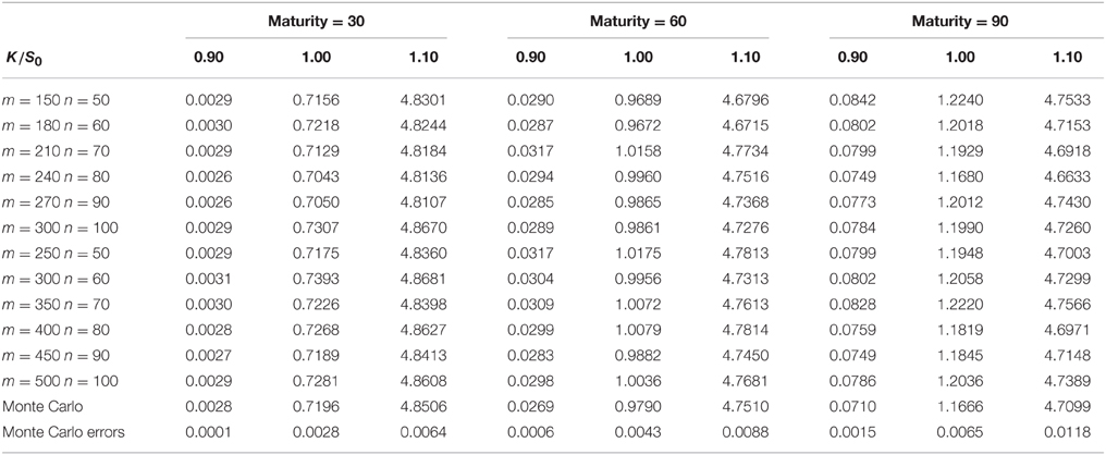
Table 2. European put options in the CTS-GARCH framework.

TABLE 3

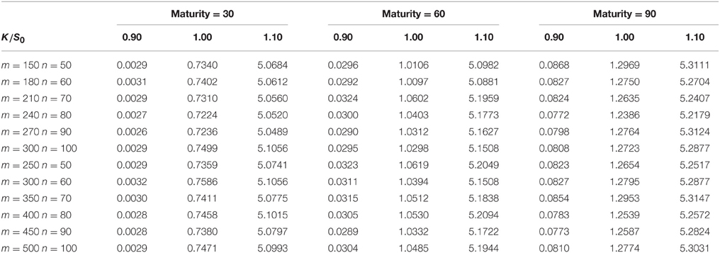
Table 3. American put options in the NTS-GARCH framework.

TABLE 4

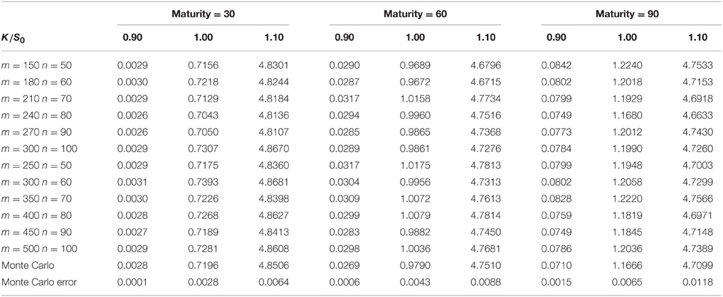
Table 4. European put options in the NTS-GARCH framework.

From these results one can observe that the results of Markov chain method with large m and n and the ones of Monte Carlo correspond roughly in two decimal place. Most of the prices in Tables 1, 3 is greater than the corresponding prices in Tables 2, 4, since the American option is always more expensive than the European option. The convergence of American options is not as fast as the one of European options. This because that small differences in accuracy might change the optimal execution time which would make the price different. We do not compare the American option price with the well known least squares method because the latter is not accurate when the option is out of money. Even for the options which are in the money, the polynomial approximation is only accurate in a small range of stock prices. We would expect more extreme values in GARCH model with heavy tailed distributions. This might make the least square approach more inaccurate.

The fluctuations in the prices are the results of discretizing the stock price and volatility. By comparing the results with the Duan's Normal GARCH model one can find that we need larger m and n to get an acceptable result. This is because we need more grids in a wider interval to approximate the cumulative distribution functions of heavy tailed distributions. In addition, the rate of convergence become slow when the maturity increases. As Duan and Simonato [19] suggested in his paper, the Markov chain method might not be good for options with long maturity.

4.2. Empirical Analysis

In this section, we illustrate the calibration of risk neutral parameters using Markov chain method. As an example, we consider the SPX put option on June 13, 2013 whose moneyness is between 0.9 and 1.1, and whose maturity is 30 days. There are 46 options meet these conditions, the strike price of which ranges from 1480 to 1740. The initial price of S&P 500 index is 1640.42.

The first step is to estimate the parameters under market measure ℙ. The maximum likelihood estimation (MLE) of ARMA(1,1)-GARCH(1,1) with Gaussian innovation is widely known. For non-Gaussian innovations, we can use the quasi maximum likelihood estimator (QMLE). That is, we first estimate the ARMA(1,1)-GARCH(1,1) parameters under Gaussian assumption. Then we will get a sequence of residuals which are assumed to be i.i.d. Finally we use other distributions like CTS or NTS to fit these i.i.d residuals. The convergence of QMLE is studied by Lee and Hansen [27] and Lumsdaine [28]. We select 2 years log daily returns of S&P 500 index as our sample. The data is downloaded from Yahoo finance. The estimated parameters are given by Tables 5–7.

TABLE 5

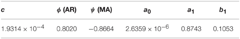
Table 5. ARMA(1,1)-GARCH(1,1) parameters.

TABLE 6

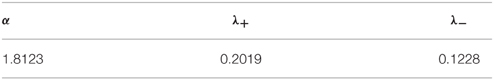
Table 6. Standard CTS parameters.

TABLE 7

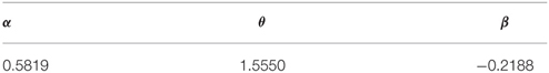
Table 7. Standard NTS parameters.

Then we can compute the risk neutral parameters in two ways. The first way is to minimize the relative entropy between ℙ and ℚ, as described in Section 2.3. The relative entropy is given by Equation (10), which is computed numerically. Here we assume that the GARCH parameters do not change under ℚ. This assumption is widely used in most GARCH option pricing papers, see Duan [8], Stentoft [29], Kim et al. [6] and Rachev et al. [20]. The results of the minimization are shown in Tables 8, 9.

TABLE 8

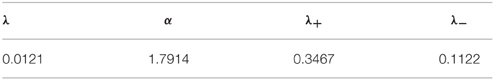
Table 8. Minimal entropy parameters (CTS).

TABLE 9

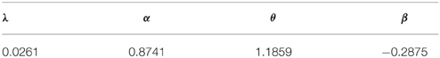
Table 9. Minimal entropy parameters (NTS).

Using these parameters we compute the option price via Markov chain method. We compute the average absolute error (AAE), average percentage error (APE), average relative percentage error (ARPE) and root mean square error (RMSE), which are give by Table 10.

TABLE 10

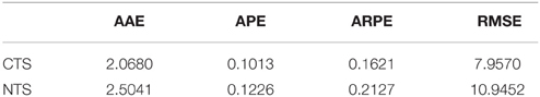
Table 10. Errors of minimal entropy measure.

The second way is to calibrate the risk neutral measure using realized option price, that is, to find the measure which minimizes the errors between model prices and market prices. In this paper we use RMSE to measure the error. The calibrated parameters and their errors are given by Tables 11–13. One can observe that the calibrated risk neutral parameters are different from the minimal entropy parameters.

TABLE 11

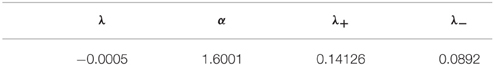
Table 11. Calibrated parameters (CTS).

TABLE 12

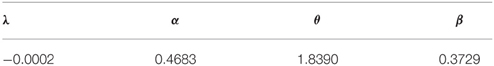
Table 12. Calibrated parameters (NTS).

TABLE 13

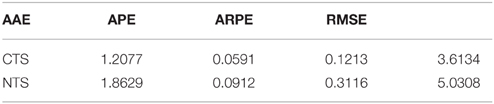
Table 13. Errors of minimal entropy measure.

We find that in both risk neutral measures CTS outperform NTS. However, it is not enough to conclude that CTS is better than NTS based on this specific example. In fact, NTS is usually good in the high dimensional case since it is a subordinated distribution and has a natural multivariate extension. It is also not enough to conclude that minimal-entropy measure is not the real risk neutral measure. The minimal entropy approach is based on the assumption that the risk neutral world is very close to the real one. The calibrated parameters might overfit the model if the option is not volatile. Here we use this method because it provides a convenient way to consider risk neutral model under Markov chain framework. Selecting the best measure in the incomplete market is out of the scope of this paper.

5. Conclusion

In this paper we employ the Markov chain approximation method to compute the value of American-style options under TS-GARCH model. We apply the minimal entropy approach to find the “best” equivalent martingale measure in an incomplete market. This risk neutral measure also allows us to compute the Markov chain method in efficiently. For heavy-tailed distributions, we use the quantile instead of the variance of the distribution to determine the range of the discrete Markov chain. We also consider the rate of tail decay to find the step size of the discretized stock prices. The convergence of the Markov chain approximation for TS-GARCH models can be proved due to the absolute continuity of TS-distribution functions. The Markov chain method is a good alternative for the least square approximation, since the latter one is less accurate when the option is out of the money and when extreme event happens. Furthermore, although the Markov chain approach for TS-GARCH is slower than the one for normal GARCH, TS-GARCH model performs much better than normal GARCH in option pricing since it has more degrees for freedom to capture the heavy-tails in financial markets.

Conflict of Interest Statement

The authors declare that the research was conducted in the absence of any commercial or financial relationships that could be construed as a potential conflict of interest.

References

1. Mandelbrot BB. New methods in statistical economics. J Pol Econ. (1963) 71:421–40. doi: 10.1086/258792

PubMed Abstract | CrossRef Full Text | Google Scholar

2. Koponen I. Analytic approach to the problem of convergence of truncated lévy flights towards the gaussian stochastic process. Phys Rev E. (1995) 52:1197–9. doi: 10.1103/PhysRevE.52.1197

PubMed Abstract | CrossRef Full Text | Google Scholar

3. Boyarchenko SI, Levendorskiĭ SZ. Option pricing for truncated lévy processes. Int J Theor Appl Finance. (2000) 3:549–52. doi: 10.1142/S0219024900000541

CrossRef Full Text

4. Carr P, Geman H, Madan D, Yor M. The fine structure of asset returns: an empirical investigation. J Bus. (2002) 75:305–32. doi: 10.1086/338705

CrossRef Full Text | Google Scholar

5. Barndorff-Nielsen OE, Levendorskii S. Feller processes of normal inverse gaussian type. Quant Finance. (2001) 1:318–31. doi: 10.1088/1469-7688/1/3/303

CrossRef Full Text | Google Scholar

6. Kim YS, Rachev ST, Chung DM, Bianchi ML. The modified tempered stable distribution, GARCH-models and option pricing. Probab Math Stat. (2009) 29:91–117.

Google Scholar

7. Kim YS, Rachev ST, Bianchi ML, Fabozzi FJ. Financial market models with lévy processes and time-varying volatility. J Bank Finance. (2008) 32:1363–78. doi: 10.1016/j.jbankfin.2007.11.004

CrossRef Full Text | Google Scholar

8. Duan JC. The GARCH option pricing model. Math Finance. (1995) 5:13–32. doi: 10.1111/j.1467-9965.1995.tb00099.x

PubMed Abstract | CrossRef Full Text | Google Scholar

9. Duan JC. Augmented GARCH (p,q) process and its diffusion limit. J Econ. (1997) 79:97–127. doi: 10.1016/S0304-4076(97)00009-2

CrossRef Full Text | Google Scholar

10. Kallsen J, Taqqu MS. Option Pricing in ARCH-type models. Math Finance. (1998) 8:13–26. doi: 10.1111/1467-9965.00042

CrossRef Full Text | Google Scholar

11. Heston L, Nandi S. A closed-form GARCH option valuation model. Rev Finacial Stud. (2000) 13:585–625. doi: 10.1093/rfs/13.3.585

CrossRef Full Text | Google Scholar

12. Christoffersen P, Jacobs K, Ornthanalai C. GARCH option valuation: theory and evidence. J Derivat. (2013) 21:8–41. doi: 10.2139/ssrn.2054859

CrossRef Full Text | Google Scholar

13. Menn C, Rachev ST. A GARCH option pricing model with α-stable innovations. Eur J Oper Res. (2005) 163:201–09. doi: 10.1016/j.ejor.2004.01.009

CrossRef Full Text | Google Scholar

14. Menn C, Rachev ST. Smoothly truncated stable distributions, GARCH-models, and option pricing. Math Methods Oper Res. (2009) 69:411–38. doi: 10.1007/s00186-008-0245-6

CrossRef Full Text | Google Scholar

15. Stentoft L. American option pricing using GARCH models and the normal inverse Gaussian distribution. J Financ. Econom. (2008) 6:540–82. doi: 10.1093/jjfinec/nbn013

CrossRef Full Text | Google Scholar

16. Kim YS, Rachev ST, Bianchi ML, Fabozzi FJ. Tempered stable and tempered infinitely divisible GARCH models. J Bank Finance (2010) 34:2096–109. doi: 10.1016/j.jbankfin.2010.01.015

CrossRef Full Text | Google Scholar

17. Longstaff FA, Schwartz ES. Valuing American options by simulation: a simple least-squares approach. Rev Financ Stud. (2001) 14:113–48. doi: 10.1093/rfs/14.1.113

CrossRef Full Text | Google Scholar

18. Ritchken P, Trevor R. Pricing options under generalized GARCH and stochastic volatility processes. J Finance. (1999) 54:377–402. doi: 10.1111/0022-1082.00109

CrossRef Full Text | Google Scholar

19. Duan JC, Simonato JG. American option pricing under GARCH by a Markov chain approximation. J Econ Dyn Control. (2001) 25:1689–718. doi: 10.1016/S0165-1889(00)00003-8

CrossRef Full Text | Google Scholar

20. Rachev ST, Kim YS, Bianchi ML, Fabozzi FJ. Financial Model with Levy Processes and Volatility Clustering. Hoboken, NJ: John Wiley & Sons (2011).

Google Scholar

21. Bouchard B, Warin, X. Monte-Carlo valuation of American options: facts and new algorithms to improve existing methods. In: Carmona RA, Del Moral P, Hu P, Oudjane N, editors. Numerical Methods in Finance. Berlin; Heidelberg: Springer (2012). p. 215-255.

22. Cont R, Tankov P. Financial Modelling with Jump Processes. London: Chapman & Hall / CRC (2004).

23. Gerber FA, Shiu ESW. Option pricing by Esscher transforms. Trans Soc Actuar. (1994) 46:99–191.

24. Gerber FA, Shiu ESW. Actuarial bridges to dynamic hedging and option pricing. Insur Math Econ. (1996) 18:183–531. doi: 10.1016/0167-6687(96)85007-4

CrossRef Full Text | Google Scholar

25. Fujiwara T, Miyahara Y. The minimal entropy martingale measures for geometric lévy processes. Finance Stoch. (2003) 7:509–31. doi: 10.1007/s007800200097

CrossRef Full Text | Google Scholar

26. Kim YS, Rachev S, Bianchi ML, Fabozzi FJ. Computing VaR and AVaR in infinitely divisible distributions. Probab Math Stat. (2009) 30:223–45. doi: 10.2139/ssrn.1400965

CrossRef Full Text | Google Scholar

27. Lee SW, Hansen BE. Asymptotic theory for the GARCH (1, 1) quasi-maximum likelihood estimator. Econom. Theory (1994) 10:29–52. doi: 10.1017/S0266466600008215

CrossRef Full Text | Google Scholar

28. Lumsdaine RL. Consistency and asymptotic normality of the quasi-maximum likelihood estimator in IGARCH (1, 1) and covariance stationary GARCH (1, 1) models. Econometrica (1996) 64:575–596. doi: 10.2307/2171862

CrossRef Full Text | Google Scholar

29. Stentoft L. Pricing American options when the underlying asset follows GARCH processes. J Empir Finance (2005) 12:576–611. doi: 10.1016/j.jempfin.2004.08.001

CrossRef Full Text | Google Scholar