Regularization by the Linear Functional Strategy with Multiple Kernels

1. Introduction

In this paper we are concerned with the so-called “supervised learning” or “learning from examples” problem, which refer to the task of predicting an output, say v ∈ V ⊂ ℝ, of a system under study from a previously unseen input u ∈ U ⊂ ℝ^d on the basis of the set of training examples, that is a set of input-output pairs z_i = (u_i, v_i), i = 1, 2, …, m, observed in the same system.

A kernel based algorithm consists in learning a function x : U → ℝ in some Reproducing Kernel Hilbert Space (RKHS) X = X_K generated by a suitable Mercer (continuous, symmetric and positive semidefinite) kernel K : U × U → ℝ that assigns to each input u ∈ U an output x(u). The prediction error is measured by the value of a chosen loss function l(v, x(u)), say square-loss l(v, x(u)) = (v − x(u))².

In the context of kernel based supervised learning a regularization is a compromise between the attempt to fit given data $z={\left\{z_i=(u_i,v_i)\right\}}_{i=1}^m\subset U\times V$ and the desire to reduce the complexity of a data fitter x ∈ X_K. For example, a Tikhonov-type kernel based learning algorithm in its rather general form defines a predictor x(u) = x_z(u) = x(K; u) ∈ X_K as the minimizer of the sum:

$\begin{array}{ll}{T}_{\alpha ,z}(x;K)=\frac{1}{m}{\displaystyle \sum _{i=1}^m}l(v_i,x(u_i))+\alpha \left|\right|x|{|}_{X_K}^2,& (1)\end{array}$

where the complexity is measured by the norm ||·||_XK in RKHS generated by a kernel K, and the above-mentioned compromise is governed by the value of the regularization parameter α.

As it has been mentioned in Michelli and Pontil [1], a challenging and central problem of kernel based learning is the choice of the kernel K itself. Recent applications (see [2, 3]) have shown that using multiple kernels instead of a single one can enhance the interpretability of the predictor x(u) = x(K; u) and improve performances. In such cases, a convenient approach is to consider that the kernel K is actually a combination of predefined basis kernels:

$\begin{array}{rc}K={\displaystyle \sum _{j=1}^p}{d}_j{K}_j,& (2)\end{array}$

where each basis kernel K_j may either use the full set of variables (u¹, u², …, u^d) describing the input u = (u¹, u², …, u^d) ∈ ℝ^d or subsets of variables stemming from different data sources. Defining both the minimizer x(K; u) of T_{α, z}(x; K) and the weights Equation (2), d_j, j = 1, 2, …, p, in a single optimization problem is known as the Multiple Kernel Learning (MKL).

A generalized representer theorem by Schölkopf et al. [4] tells us that a large class of optimization problems Equation (1) with RKHS have solutions expressed as kernel expansions in terms of the training data z. More precisely, for each K = K_j, j = 1, 2, …, p, the minimizer x(K_j; u) belongs to the finite-dimensional linear subspace spanned by the functions K_j(u, u_i), i = 1, 2, …, m. Therefore, MKL-predictor x_z(u) can be written as:

$\begin{array}{ll}{x}_z(u)={\displaystyle \sum _{i=1}^m}{\displaystyle \sum _{j=1}^p}{b}_{i,j}{K}_j(u_i,u).& (3)\end{array}$

There is a significant amount of work in the MKL-literature. For example, the survey [5] reviews a total of 96 references. A comparison of existing MKL-algorithms performed in that survey shows that through there may not be large differences in terms of accuracy, there is difference between MKL-algorithms in complexity as given by the training time, for example.

Similar accuracies of different MKL-algorithms can be, at least partially, explained by the fact that all minimizers x_j(K_j; ·) of Equation (1) for K = K_j, j = 1, 2, …, p belong to the direct sum X_K+ of RKHS X_Kj, j = 1, 2, …, p, and a classical result [6] says that X_K+ is a RKHS generated by the kernel K₊ = K₁ + K₂ + … +K_p.

The differences in training time originate from different optimization algorithms used for learning the weights d_j, j = 1, 2, …, p. The so-called one-step methods calculate both the combination weights d_j, j = 1, 2, …, p and the parameters of the minimizer x(K; u) in a single run. However, these methods use optimization approaches, such as semi-definite programming (SDP) [7], second order conic programming (SOCP) [8], or quadratically constrained quadratic programming (QCQP) [9], which have high computational complexity especially for large number of samples.

Two-step, or wrapper methods address the MKL-problem by iteratively solving a single learning problem, such as Equation (1), for a fixed combination of basis kernels, and then update the kernel weights. Such methods run usually much faster than the one-step methods and therefore there is a rich variety of them. Just to mention some of them we refer to Semi-Infinite Linear Program (SILP) approach [10], SimpleMKL method [11] performing a reduced gradient descent on the kernel weights, LevelMKL algorithm [12], HessianMKL [13], replacing the gradient descent in SimpleMKL by the Newton update, and some others [1, 14].

The time complexity of these two-step methods depends on the number of iterations of an algorithm until the stopping criterion is fulfilled. In this context our idea is to use the so-called Linear Functional Strategy (LFS) [15], originally proposed for single-kernel ranking learning, allowing to find the coefficients of the linear combination in one step by using the given training set. In this paper we extend this idea to the MKL setting, namely we analyze the linear functional strategy for combining the x_j(K_j; u) ∈ X_Kj into a new predictor.

The paper is organized as follows: in the next section we present the main theoretical results. Then, we compare the proposed method with two other MKL-learning approaches, namely SimpleMKL and SpicyMKL [16]. Finally, we discuss some open questions and further research directions.

2. Main Results

If we accept the basic statistical learning assumptions, namely that the inputs u and the outputs v are assumed to be related by a conditional probability distribution ρ(v|u) of v given u, and the input u is also assumed to be random and governed by an unknown marginal probability ρ_U on U so that there is an unknown probability distribution ρ(u, v) = ρ_U(u)ρ(v|u) on the sample space U × V from which the data forming the training set are drawn independently, then the “ideal predictor” x^† is assumed to belong to the space X = L₂(U, ρ_U) of square integrable functions with respect to ρ_U and can be defined as the element minimizing the expected prediction risk:

$E(f)={\displaystyle {\int }_{U\times V}{\left(x(u)-v\right)}^{2}d\rho (u,v).}$

Moreover, in such set-up x^† can be written explicitly in the form:

$x^{†}(u)={\displaystyle {\int }_{V}vd\rho (v|u),u\in U.}$

As one can see from the above formula, x^† cannot be used in practice, since the conditional probability ρ(v|u) is not assumed to be known.

Our idea is to construct a MKL-predictor Equation (3) in the form:

$\begin{array}{ll}{x}_z(u)={\displaystyle \sum _{j=1}^p}{c}_j{x}_j(K_j;u),& (4)\end{array}$

where c_j are the unknown coefficients. It is clear that the best choice of the coefficient vector $c=\overline{c}$ should minimize the distance:

$\begin{array}{ll}{\Vert x^{†}-{\displaystyle \sum _{j=1}^p{c}_j}{x}_j(K_j;u)\Vert }_X^2,& (5)\end{array}$

and it is easy to see that such $\overline{c}$ solves the following linear system of equations:

$\begin{array}{ll}G\overline{c}=g& (6)\end{array}$

with the Gram matrix $G={({\langle x_l(K_l;·),x_j(K_j;·)\rangle }_{L_2(U,{\rho }_U)})}_{l,j=1}^p$ and the right-hand-side vector $g={({\langle x^{†},x_l(K_l;·)\rangle }_{L_2(U,{\rho }_U)})}_{l=1}^p$. Clearly, the right-hand side g is inaccessible due to the involvement of the unknown predictor x^†. Furthermore, the components of the matrix G are not accessible, since the measure ρ_U is also unknown.

To simplify further discussion, we assume that $x^{†}\in X_{K_{+}}$, which is not a big restriction if at least one of K_j is the so-called universal kernel [17], and consider the inclusion operator I₊ of X_K+ into L₂(U, ρ_U) and the sampling operator $S_z:X_{K_{+}}\to {ℝ}^m$ defined by $S_{z}x=(x(u_1),x(u_2),\dots ,x(u_m))\in {ℝ}^m$. Then under rather general assumptions (see 18) with high probability 1 − η we have:

$\begin{array}{l}{\Vert I_{+}^{*}{I}_{+}-S_z^{*}{S}_z\Vert }_{X_{K_{+}}\to X_{K_{+}}}\le c_1{m}^{-1/2}\log \frac{1}{\eta },{\Vert S_z^{*}{S}_z{x}^{†}-S_z^{*}v\Vert }_{X_{K_{+}}}\\ \le c_2{m}^{-1/2}\log \frac{1}{\eta },& (7)\end{array}$

where $S_z^{*}:{ℝ}^m\to X_{K_{+}}$, $I_{+}^{*}:L_2(U,{\rho }_U)\to X_{K_{+}}$ are adjoints of S_z and I₊; v = (v₁, v₂, …, v_m) is the vector of the outputs used for training; c₁, c₂ are certain multipliers which do not depend on m, η.

With the use of Equation (7) we can approximate the components of the vector g and the Gram matrix G as:

$\begin{array}{l}{\langle x^{†},x_l(K_l;·)\rangle }_{L_2(U,{\rho }_U)}={\langle I_{+}{x}^{†},I_{+}{x}_l(K_l;·)\rangle }_{L_2(U,{\rho }_U)}={\langle I_{+}^{*}{I}_{+}{x}^{†},x_l(K_l;·)\rangle }_{X_{K_{+}}}\\ ={\langle S_z^{*}{S}_z{x}^{†},x_l(K_l;·)\rangle }_{X_{K_{+}}}+O(m^{-1/2}\log \frac{1}{\eta })={\langle S_z^{*}v,x_l(K_l;·)\rangle }_{X_{K_{+}}}\\ +O(m^{-1/2}\log \frac{1}{\eta })={\langle v,S_z{x}_l(K_l;·)\rangle }_{{ℝ}^m}+O(m^{-1/2}\log \frac{1}{\eta })\\ =m^{-1}{\displaystyle \sum _{i=1}^m{v}_i}{x}_l(K_l;u_i)+O(m^{-1/2}\log \frac{1}{\eta }),& (8)\end{array}$

$\begin{array}{ll}{\langle x_l(K_l;·),x_j(K_j;·)\rangle }_{L_2(U,{\rho }_U)}=m^{-1}{\displaystyle \sum _{i=1}^m{x}_l}(K_l;u_i)x_j(K_j;u_i)+O(m^{-1/2}\log \frac{1}{\eta }).& (9)\end{array}$

In view of these relations, we state the main result of this section through the following theorem:

Theorem 1. Let $V\subset \left[-b,b\right],x^{†}\in X_{K_{+}}$ and K_j(u, u) ≤ c, u ∈ U, j = 1, 2, …, p. Consider

$\begin{array}{l}\tilde{G}=\frac{1}{m}{\left({\displaystyle \sum _{i=1}^m{x}_l}(K_l;u_i)x_j(K_j;u_i)\right)}_{j,l=1}^p,\\ \tilde{g}=\frac{1}{m}{\left({\displaystyle \sum _{i=1}^m{v}_i}{x}_j(K_j;u_i)\right)}_{j=1}^p,\end{array}$

and assume that $\tilde{G}$ is invertible. Then for MKL-approximant:

$\begin{array}{ll}{x}_z(u)={\displaystyle \sum _{j=1}^p{\tilde{c}}_j}{x}_j(K_j;u),\tilde{c}={({\tilde{c}}_j)}_{j=1}^p={\tilde{G}}^{-1}\tilde{g}.& (10)\end{array}$

with confidence 1 − η it holds:

$\begin{array}{l}{\Vert x^{†}-x_z\Vert }_{L_2(U,{\rho }_U)}=\underset{c_j}{\min }{\Vert x^{†}-{\displaystyle \sum _{j=1}^p{c}_j}{x}_j(K_j;u)\Vert }_{L_2(U,{\rho }_U)}\\ +O(m^{-1/2}\log (1/\eta )),\end{array}$

where a coefficient implicit in O-symbol does not depend on m.

Proof. Formulas (8, 9) tells us that with confidence 1 − η it holds:

$\begin{array}{l}{\Vert G-\tilde{G}\Vert }_{{ℝ}^p\to {ℝ}^p}=O(m^{-1/2}\log \frac{1}{\eta }),{\Vert g-\tilde{g}\Vert }_{{ℝ}^p}\\ =O(m^{-1/2}\log \frac{1}{\eta }).& (11)\end{array}$

If ${\tilde{G}}^{-1}$ exists then in view of (11) it is natural to assume that for sufficiently large m with confidence 1 − η we have:

$\begin{array}{ll}{\Vert G-\tilde{G}\Vert }_{{ℝ}^p\to {ℝ}^p}<\frac{1}{{\Vert {\tilde{G}}^{-1}\Vert }_{{ℝ}^p\to {ℝ}^p}}.& (12)\end{array}$

This assumption allows the application of the well-known Banach theorem on inverse operators (see 19, V. 4.5), which tells that:

$\begin{array}{ll}{\Vert G^{-1}\Vert }_{{ℝ}^p\to {ℝ}^p}\le \frac{{\Vert {\tilde{G}}^{-1}\Vert }_{{ℝ}^p\to {ℝ}^p}}{1-{\Vert {\tilde{G}}^{-1}\Vert }_{{ℝ}^p\to {ℝ}^p}{\Vert G-\tilde{G}\Vert }_{{ℝ}^p\to {ℝ}^p}}=O(1).& (13)\end{array}$

Consider the vectors $\overline{c}=G^{-1}g,\tilde{c}={\tilde{G}}^{-1}\tilde{g}$. Then from (11) to (13) it follows that:

$\begin{array}{ll}{\Vert \overline{c}-\tilde{c}\Vert }_{{ℝ}^p}=O(m^{-1/2}\log \frac{1}{\eta }),& (14)\end{array}$

and

$\begin{array}{l}{\Vert x^{†}-x_z\Vert }_{L_2(U,{\rho }_U)}\le \underset{c_j}{\min }{\Vert x^{†}-{\displaystyle \sum _{j=1}^p{c}_j}{x}_j(K_j;u)\Vert }_{L_2(U,{\rho }_U)}\\ +p{\Vert \overline{c}-\tilde{c}\Vert }_{{ℝ}^p}\underset{j}{\max }{\Vert x_j(K_j;u)\Vert }_{L_2(U,{\rho }_U)}& (15)\end{array}$

Moreover, since x_j(K_j; ·) is the minimizer of Equation (1) for K = K_j and l(v, x(u)) = (v − x(u))², from Proposition 4.1 [20] it follows that ||x_j(K_j; ·)||_{L2(U, ρU)} are uniformly bounded such that for α from the range of interest, i.e., for α ≥ m⁻¹, we have $\left|\right|x_j(K_j;·)|{|}_{L_2(U,{\rho }_U)}\le d|\left|x^{†}\right|{|}_{L_2(U,{\rho }_U)}$, where $d=O\left(log\frac{1}{\eta }\right)$ and does not depend on m, j.

Then the statement of the theorem follows from (14) to (15). □

Remark 1. In Theorem 1 the Gram matrix $\tilde{G}$ is supposed to be well-conditioned. In principle, one may control this by excluding those members of the family {x_j(K_j; u), j = 1, 2, …, p} that are close to be linear dependent of others. A preconditioning method for such a control has been discussed, for example, in Chen et al. [21] (see Remark 3.1 there).

Theorem 1 tells us that the effectively constructed linear combination of the candidates x_j(K_j; ·), j = 1, 2, …, p, is almost as accurate as the best linear aggregator of them.

A simple algorithmic sketch of such almost the best aggregator is provided below:

ALGORITHM

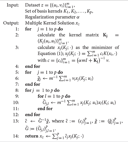
Algorithm of the Linear Functional Strategy for MKL

In the next Section we present some numerical experiments illustrating the performance of the proposed algorithm. We will denote the MKL-predictor Equations (4), (10) constructed via linear functional strategy (LFS) in the above mentioned way by MKL-LFS.

3. Numerical Illustrations

It is interesting to compare MKL-LFS with the other two MKL-algorithms, named SimpleMKL and SpicyMKL, that have been proposed respectively in Rakotomamonjy et al. [11] and Suzuki and Tomioka [16]. We choose the first one, SimpleMKL, for comparison, because the experimental results reported in Rakotomamonjy et al. [11] show that this algorithm converges rapidly and that its efficiency compares favorably to other MKL algorithms. It is also important that a SimpleMKL toolbox based on Matlab code is available at http://www.mloss.org and, therefore, we are able to put MKL-LFS and SimpleMKL side by side. Moreover, the second competitor, SpicyMKL, uses SimpleMKL on the set-up stage.

The second algorithm, SpicyMKL, has been chosen because it is reported to be the fastest one among all other algorithms, and in particular, much faster than SimpleMKL.

To perform the comparison of SimpleMKL and SpicyMKL with MKL-LFS, we use the same experimental set-up as in Rakotomamonjy et al. [11]. More precisely, the performance evaluation is made on five data sets from the UC Irvine Machine Learning Repository: Liver, Wpbc, Ionosphere, Pima, Sonar. For each data set, the compared algorithms were run 20 times with train and test sets selected differently for each run by SimpleMKL toolbox (70% of the data set for training and 30% for testing the performance).

The SpicyMKL algorithm has been tuned in order to run its fastest version, namely with the logistic regression loss and elastic net regularization. The tuning parameters were taken the same as suggested in Suzuki and Tomioka [16].

The candidate kernels K_j, j = 1, 2, …, p are the Gaussian kernels with 10 different bandwidths, on all variables u = (u¹, u², …, u^d) and in each single variable u^j, j = 1, 2, …, d; these kernels are accompanied by the polynomial kernels of degree 1–3, again on all and on each single variable. So, the number p of kernel candidates depends on the dimension d of the input variable u = (u¹, u², …, u^d). For each of the considered data sets the value p is indicated in Table 1.

TABLE 1

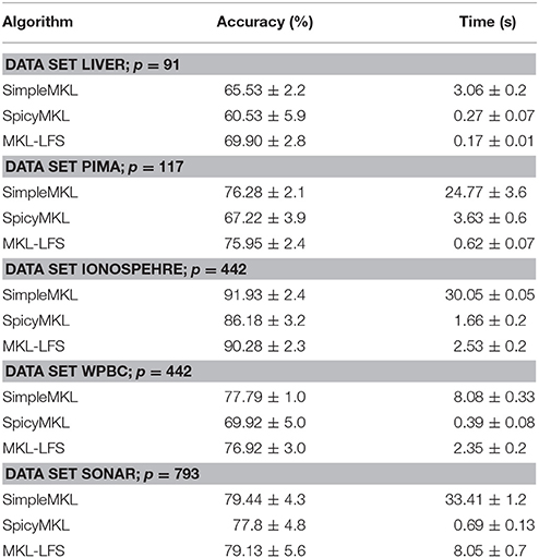
Table 1. Average performance measures for SimpleMKL, SpicyMKL, and MKL-LFS.

The table also reports the average values of the training time and the accuracy over 20 runs of the compared algorithms.

Since the above mentioned five data sets are associated with the classification learning task (i.e., v_i = ±1), the algorithms accuracy is measured by the percentage of the correctly classified examples (i.e., when sign(x(u)) = sign(v)) from the part of the data set that has not been used for training.

Table 1 shows that SimpleMKL and MKL-LFS are nearly identical in the performance accuracy, while SpicyMKL is less effective against this criterion. If we look at the computation time reported in Table 1, clearly, on all data sets MKL-LFS is much fasted than SimpleMKL. On the other hand, SpicyMKL is faster than two other algorithms on the sets, where the number of kernels is large, but the size of the training set is moderate. The same feature was observed in Suzuki and Tomioka [16]: the algorithm SpicaMKL is efficient when the number of unknown variables is much larger than the number of samples. It should be noted that the MKL-LFS does not suffer from this restriction.

4. Discussion

For the purpose of comparing we follow [11] and put SimpleMKL and MKL-LFS side by side for a fixed value of the so-called hyperparameter C = 100, that corresponds to α = 1/2C = 0.005 in Equation (1). Moreover, for SpicyMKL two regularization parameters need to be selected (in our tests they are fixed as proposed in [16]). At the same time, we expect that the accuracy of MKL-LFS may be improved by combining in Equation (4) the minimizers x_j(K_j; ·) of Equation (1) corresponding to different α = α(K_j), which are properly chosen for each K = K_j, j = 1, 2, …, p. We will derive such an algorithm in the near future end expect that the speed gain observed in Table 1 for MKL-LFS allows us to implement such a posteriori choice of α effectively in time.

Moreover, our method, in principle, is not restricted to Tikhonov-type regularizations only, which is known to be affected by saturation [22]. One may potentially use any of the regularization methods, such as Landweber iteration, for example, for computing the predictors x_j(K_j, ·). In view of this, we plan to develop in the near future the MKL algorithm based on the so-called general regularization framework for learning [20].

Author Contributions

All authors listed, have made substantial, direct and intellectual contribution to the work, and approved it for publication.

Funding

The authors gratefully acknowledge the support of the Austrian Science Fund (FWF), project I1669, and of the consortium AMMODIT funded within EU H2020-MSCA-RICE.

Conflict of Interest Statement

The authors declare that the research was conducted in the absence of any commercial or financial relationships that could be construed as a potential conflict of interest.

References

1. Michelli CA, Pontil M. Learning the kernel function via regularization. J Mach Learn Res. (2005) 6:1099–1125.

PubMed Abstract

2. Lanckriet GRG, De Bie T, Cristianini N, Jordan MI, Noble WS. A statistical framework for genomic data fusion. Bioinformatics (2004) 20:2626–35. doi: 10.1093/bioinformatics/bth294

PubMed Abstract | CrossRef Full Text | Google Scholar

3. Wu Q, Ying Y, Zhou DX. Multi-kernel regularized classifiers. J Complex. (2007) 23:108–34. doi: 10.1016/j.jco.2006.06.007

CrossRef Full Text | Google Scholar

4. Schölkopf B, Herbrich R, Smola AJ. A Generalized Representer Theorem. Comput Learn Theory Lect Notes Comput Sci. (2001) 2111:416–26. doi: 10.1007/3-540-44581-1_27

PubMed Abstract | CrossRef Full Text | Google Scholar

5. Gönen M, Alpaydin E. Multiple kernel learning algorithms. J Mach Learn Res. (2011) 12:2211–68.

PubMed Abstract | Google Scholar

6. Aronszajn N. Theory of reproducing kernels. Trans Am Math Soc. (1950) 68:337–404. doi: 10.1090/S0002-9947-1950-0051437-7

PubMed Abstract | CrossRef Full Text | Google Scholar

7. Lanckriet GRG, Cristianini N, Bartlett P, Ghaoui LE, Jordan MI. Learning the kernel matrix with semidefinite programming. J Mach Learn Res. (2004) 5:27–72.

PubMed Abstract | Google Scholar

8. Bach FR, Lanckriet GRG, Jordan MI. Multiple kernel learning, conic duality, and the SMO algorithm. In: Proceedings of the Twenty-first International Conference on Machine Learning. ICML '04. New York, NY: ACM (2004). p. 6. Available online at: http://doi.acm.org/10.1145/1015330.1015424

9. Conforti D, Guido R. Kernel based support vector machine via semidefinite programming: application to medical diagnosis. Comput Oper Res. (2010) 37:1389–94. doi: 10.1016/j.cor.2009.02.018

CrossRef Full Text | Google Scholar

10. Sonnenburg S, Rätsch G, Schäfer C, Schölkopf B. Large scale multiple kernel learning. J Mach Learn Res. (2006) 7:1531–65.

PubMed Abstract | Google Scholar

11. Rakotomamonjy A, Bach FR, Canu S, Grandvalet Y. SimpleMKL. J Mach Learn Res. (2008) 9:2491–521.

PubMed Abstract | Google Scholar

12. Xu Z, Jin R, King I, Lyu MR. An extended level method for efficient multiple kernel learning. In: Proceedings of the 21st International Conference on Neural Information Processing Systems. NIPS'08. Curran Associates Inc. (2008). p. 1825–32. Available online at: http://dl.acm.org/citation.cfm?id=2981780.2982009

13. Chapelle O, Rakotomamonjy A. Second order optimization of kernel parameters. In: Kernel Learning Workshop: Automatic Selection of Optimal Kernels. (2008). Available online at: http://www.cs.nyu.edu/learning_kernels/abstracts/nips_wshp.pdf

14. Naumova V, Pereverzyev SV, Sivananthan S. Extrapolation in variable RKHSs with application to blood glucose reading. Inverse Prob. (2011) 27:13. doi: 10.1088/0266-5611/27/7/075010

CrossRef Full Text | Google Scholar

15. Kriukova G, Panasiuk O, Pereverzyev SV, Tkachenko P. A linear functional strategy for regularized ranking. Neural Netw. (2016) 73:26–35. doi: 10.1016/j.neunet.2015.08.012

PubMed Abstract | CrossRef Full Text | Google Scholar

16. Suzuki T, Tomioka R. SpicyMKL: a fast algorithm for Multiple Kernel Learning with thousands of kernels. Mach Learn. (2011) 85:77–108. doi: 10.1007/s10994-011-5252-9

CrossRef Full Text | Google Scholar

17. Micchelli CA, Xu Y, Zhang H. Universal kernels. J Mach Learn Res. (2006) 7:2651–67.

PubMed Abstract | Google Scholar

18. Vito ED, Rosasco L, Caponnetto A, Giovannini UD, Odone F, Vito D, et al. Learning from examples as an inverse problem. J Mach Learn Res. (2005) 6:883–904.

PubMed Abstract | Google Scholar

19. Kantorovich LV, Akilov GP. Functional Analysis. Oxford: Elsevier Science (2014).

Google Scholar

20. Lu S, Pereverzyev SV. Regularization Theory for Ill-Posed Problems–Selected Topics. Berlin; Boston: Walter de Gruyter GmbH (2013).

Google Scholar

21. Chen J, Pereverzyev SS, Xu Y. Aggregation of regularized solutions from multiple observation models. Inverse Prob. (2015) 31:075005. doi: 10.1088/0266-5611/31/7/075005

CrossRef Full Text | Google Scholar

22. Engl HW, Hanke M, Neubauer A. Regularization of Inverse Problems. Dordrecht: Mathematics and Its Applications, Kluwer Academic Publishers (1996).

Google Scholar