Abstract
Computational systems biology aims at integrating biology and computational methods to gain a better understating of biological phenomena. It often requires the assistance of global optimization to adequately tune its tools. This review presents three powerful methodologies for global optimization that fit the requirements of most of the computational systems biology applications, such as model tuning and biomarker identification. We include the multi-start approach for least squares methods, mostly applied for fitting experimental data. We illustrate Markov Chain Monte Carlo methods, which are stochastic techniques here applied for fitting experimental data when a model involves stochastic equations or simulations. Finally, we present Genetic Algorithms, heuristic nature-inspired methods that are applied in a broad range of optimization applications, including the ones in systems biology.
1. Introduction
The field of optimization has become crucial in our daily life, with servers and computers solving hundreds of problems every second. From the assets to include in a portfolio, to the shape of a particular object, to the distribution of packages sent among networks and uncountable other applications, optimization problems are addressed and solved constantly.
Among the many branches of optimization, global optimization focuses on the development of techniques and algorithms to discover the best solution, according to specific criteria, when several local solutions are possible [1]. It has been intensively improved during the last decades and applied in many fields, such as mathematics, computer science, biology and statistics. These improvements have had a tangible effect in terms of accuracy of the results and time of execution, allowing the use of global optimization to solve bigger and more complex problems. In the meanwhile, the application of computer science techniques to biology has led to the establishment of computational systems biology [2, 3]. This field aims at gaining knowledge from the vast amount of data produced by the omics technologies. In addition, it resorts to dynamical representations to gain mechanistic insights into biological phenomena. Computational systems biology often requires the assistance of optimization to adequately tune its tools. For example, optimization techniques are applied to estimate model parameters, here referred as model tuning, and also for data analysis. For instance, it is used to determine biomarkers, here referred as biomarker identification, as well as to determine the optimal number of clusters in which data should be divided [3]. Since multiple local solutions to these optimization problems often occur [4, 5], we provide a concise review of three methodologies for global optimization that are successfully applied in computational systems biology [6].
The herein proposed selection of algorithms embraces three of the main optimization strategies, namely, deterministic, stochastic and heuristic [1]. We have chosen simple specific implementations that, in our opinion, help in communicating the ideas behind the algorithms and elucidate the corresponding methodologies. We avoided technical details or strict mathematical rigor to facilitate the reading also for scientists whose background is more focused on biology than in computer science or mathematics. Nevertheless, we provided technical details in the list of references, where a skilled reader can find all the resources for an in-depth coverage of the matter.
1.1. Model tuning and biomarker identification as global optimization problems
Models are here intended for in-silico simulations of biological phenomena. They are usually systems of differential or stochastic equations that quantitatively describe chemical reactions or other complex interactions. A model returns a vector of current values for all the variables. These variables can be real (e.g., average chemical concentrations) or integer (e.g., number of molecules or individuals). For example, we may consider the Lotka-Volterra model (Equation 1), also known as the prey-predator model [3].
This set of ordinary differential equations describes the population dynamics of two species in which one of them, the predators z, consume the other one, the prey y. The Lotka-Volterra model depends on four parameters: the growth rate of the prey α, the death rate of predators b, the rate at which preys are eaten by predators a and the rate at which the predator population grows as a consequence of eating prey β.
It is not unusual that some of the model parameters are unknown, such as rate constants or scaling factors. In the absence of effective methods to determine parameter estimates, a model provided with a wrong set of parameters may produce a distorted representation of the observed phenomena. This may lead to the rejection of its mechanistic description. For example, Figure 1 shows two possible outcomes of the deterministic simulation of the Lotka-Volterra model, with different sets of parameter estimates.
Figure 1
Another common application of optimization in computational systems biology is biomarker identification, which is frequently related to the problem of classifying samples measured using the omics technologies (genomics, proteomics, lipidomics, metabolomics). These techniques produce a vast amount of data and researchers are challenged to infer knowledge from it [3]. In classification, certain characteristic sample properties, such as the expression level of some genes or proteins, are selected to separate the samples. Such selected properties, here generically called features, are then used to divide samples in categories. For example, respondent and non-respondent to a particular drug or healthy and unhealthy [7, 8]. Usually a sufficiently short list of features, called biomarker, is sought to discriminate the samples. If this list of features is not optimally chosen, it may drive to poor classification accuracy.
Optimization problems can be formulated as follows:
θ is a vector of dimension p ≥ 1 and it contains the parameter estimates that are sought. A solution of the optimization problem contains those parameter estimates that minimize the function c. We generically refer at them as parameters. The cost function c, also called objective function, translates the problem in mathematical equations and it undergoes the optimization process to estimate the optimal parameters. The objective function may also depend on other variables rather than θ, as initial values, forcing functions or other variables that are not optimized. For the sake of simplicity, such values are not explicitly included in Equation (2). The objective function may depend linearly on θ, like in the case of routing or scheduling problems [9], or non-linearly, such as in many applications of computational systems biology [5]. Once these parameters are estimated, their values are fixed in the model. In contrast, the independent variables, here called just variables, remain free to vary after the optimization process. For example, in the Lotka-Volterra model (Equation 1) α, a, β, b are parameters, whereas y and z are variables. In addition, the problem may be subject to constraints, which can be bounds for the values that each θj can assume (lb and ub in Equation 2) or functional relations among the parameters (g and h). For instance, the parameters may represent biological rates or physical quantities that cannot be negative or that are admissible only inside a specific interval. In other cases, the value of certain parameters may depend on other parameters, as in the case when their sum should be smaller or equal to a certain threshold [10]. We refer to the space where the parameters θ can vary, according to constraints, as the space of parameters. This set can include continuous or discrete parameters, or both, according to the problem and the constraints on θ. If we need to optimize certain rate constants of chemical reactions, the parameter estimates are continuous values, whereas the number of genes to take into account to determine a biomarker is an integer (positive) value. During the identification of biomarkers, we may also consider a significance threshold associated to a specific statistical test. Therefore, some parameters of the problem may be continuous (significance threshold) whereas, at the same time, others may be integers (the length of the list).
In certain cases, optimization problems may be solved directly by studying the objective function. For example, if the problem depends on a limited number of parameters and variables, or the objective function is linear or convex (Figure 2A) [9, 11]. However, as soon as the number of variable increases and the function loses linearity or convexity (Figure 2B), the running time to solve the problem becomes infeasible. Thus, the need for methods that permit the systematic research for optimal solutions arises. In this article, we will focus on the case where the objective function is non-linear and non-convex and multiple solutions are possible. We have referred to the plural “methods” since there is no one-for-all method. As the No Free Lunch Theorem (NFL) states: “for any algorithm, any elevated performance over one class of problems is offset by performance over another class” [13].
Figure 2
In the following, we discuss the multi-start non-linear least squares method (ms-nlLSQ) based on a Gauss-Newton approach [14], mostly applied for fitting experimental data. We illustrate the random walk Markov Chain Monte Carlo method (rw-MCMC) [15], a stochastic technique used when a model involves stochastic equations or simulations. Finally, we present the simple Genetic Algorithm (sGA) [16], a heuristic nature-inspired method that belongs to the class of Evolutionary Algorithms. sGA is applied in a broad range of optimization applications, including model tuning and biomarker identification.
Table 1 collects some important properties of the considered methods. Under specific hypotheses [14, 15], ms-nlLSQ and rw-MCMC are proved to converge to local or global minimum, respectively. Analogously, certain implementations of sGA converge to the global solution, but solely for problems involving only discrete parameters [17, 18]. ms-nlLSQ is suitable only for problems where both model parameters and the objective function are continuous. On the other hand, rw-MCMC supports continuous and non-continuous objective functions, as well as sGA that also supports discrete parameters. All the considered optimization techniques require objective function evaluations at each iteration step, from just one evaluation in the case of rw-MCMC, to several as in the case of ms-nlLSQ and sGA.
Table 1
| ms-nlLSQ | rw-MCMC | sGA | |
|---|---|---|---|
| Convergence | Proof to local* | Proof to global* | No proof** |
| Support for continuous parameters | √ | √ | √ |
| Support for continuous objective functions | √ | √ | √ |
| Support for non-continuous objective functions | – | √ | √ |
| Support for discrete parameters | – | – | √ |
Comparison of the described algorithms.
ms-nlLSQ, multi-start non-linear least squares; rw-MCMC, random walk Markov Chain Monte Carlo; sGA, simple Genetic Algorithm.
Convergence is assured under specific hypotheses.
Certain implementations of the algorithm converge to the global solution for problems involving only discrete parameters.
2. Least squares methods
Model tuning is the estimation of model parameters to reproduce experimental time series. This problem is often formulated in the form of least squares, as in models related to diabetes [10, 19, 20], biological pathways [21–24], and pharmacokinetics/pharmacodynamics [25, 26]. Least squares problems may arise in statistical regression as well [27–32].
We denote the output of the model at a certain time instant ti as . It may be the result, for instance, of integrating differential equations. When the experimental data at the same time point is known, we can compute the residual function r, which can be defined as a vector of components
We refer to a least squares problem [33] when the objective function is obtained as the squared sum of these residuals for all the time points:
In addition, c may include weights (wi) that multiply the ri and in this case we have a weighted least squares problem [34]. This is often the case when experimental standard deviations are known and their reciprocal can be used as weights. For example, biological measures are often collected in triplicate. In such a case, experimental points can be identified by the mean of these measurements and by a dispersion index, such as the standard deviation. This helps in quantifying the confidence in the measures and the objective function will weight more the residual of those experimental points that have less uncertainty. The distance of a model output from the experimental data may always be quantified as a least squares problem. However, least squares methods mostly address problems involving continuous parameters and objective functions [14]. In the following, we embrace these assumptions.
The least squares methods exploit the properties of the particular objective function to obtain ad-hoc implementations. For example, the structure of its derivatives permits to approximate the objective function without the computation of the second order derivatives [14]. Due to this and other attractive features, many applied unconstrained problems are formulated in terms of least squares. Besides their prominent role in unconstrained optimization, some implementations allow at solving constrained problems.
According to the way in which the objective function depends on the parameters, least squares problems are divided in linear and non-linear. Linear least squares problems admit unique solution and fast solving algorithms [14], whereas non-linear least squares problems admit in general more solutions and the methods return local solutions. In order to circumvent these limitations and provide a global solution, the procedure is repeated starting from different sets of parameter estimates, hereafter called starting points. The best solution among the results of the repeated procedure is then selected to ensure that the result is global. This procedure is known as multi-start approach. However, as the number of starting point increases, the overall procedure slows down. Thus, it is crucial to determine an adequate number of initial points N, such that the space of parameters is properly explored and the problem is still tractable. In addition, multiple runs of the procedure may lead to the same set of parameter estimates, weakening the efficiency of the method.
Algorithm 1 provides a multi-start implementation for solving unconstrained non-linear least squares problems by exploiting a simple Gauss-Newton approach [33]. The global search procedure begins defining N starting points for the method. These starting points can be selected randomly in the space of parameters (Algorithm 1, line 1), or using more elaborated procedures. For example, the Latin hypercube technique samples near-randomly the space of parameters trying to reduce the clustering of points that may happen in random selection. We refer to Morris and Mitchell [35], Pronzato and Müller [36], and Viana [37] for a complete description of Latin hypercube and other sampling techniques. Once the starting points are determined, for each of them the least squares procedure is computed (Algorithm 1, lines 2–13). Remarkably, each run of this approach is independent from the others, and the procedure naturally supports parallel implementation. This may allow a consistent speed-up.
Algorithm 1
|
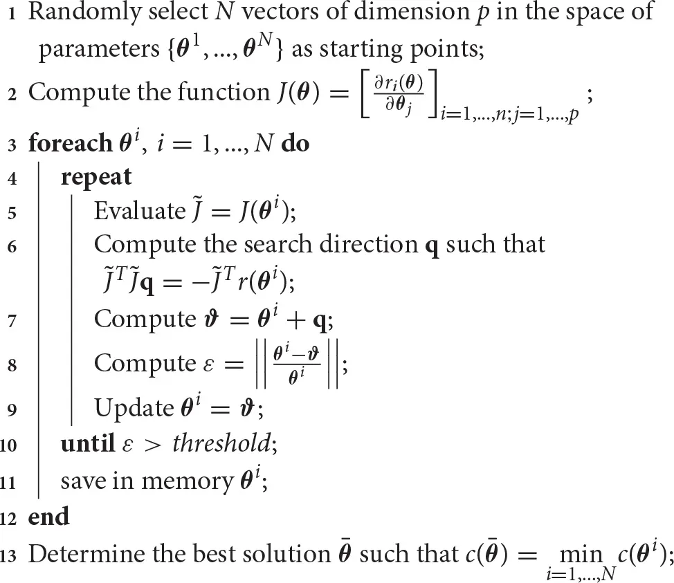 |
Multi-start non-linear least squares method based on the Gauss-Newton approach.
The here described Gauss-Newton approach for unconstrained non-linear least squares problems adopts a linearization of the objective function through a first order approximation (Algorithm 1, lines 2 and 5). At each iteration it proceeds identifying a new search direction by solving a linear least squares problem for the linearized objective function (Algorithm 1, line 6). This step requires a model simulation to compute the residuals r(θi) and an evaluation of J(θi). However, in modeling, the analytical expression of J is often unknown. In this case, the method has to approximated J(θi) at each step, requiring more model simulations [14]. Once the new search direction is determined, the parameters are updated along that direction (Algorithm 1, line 9) and these steps are repeated.
The optimization procedure runs until termination criteria are met. Among the many termination criteria [38], here we considered a common criterion that stops the procedure when the relative distance of the update is smaller than a certain threshold (Algorithm 1, line 10). Notably, the gradient of the objective function may provide termination criteria, which may be used to certify the local convergence to a stationary point. However, less computationally demanding procedures, as the one we considered, are usually preferred. When all the runs are terminated, the results are compared and the best one is selected, for instance considering the smallest value of c (Algorithm 1, line 13).
The Gauss-Newton method shows some drawbacks. In particular, this method does not support constraints on θ and requires some hypotheses to ensure the local convergence. As a consequence, more robust implementations have been proposed, including some that could manage linear or bound constraints [14, 33, 39]. Some improvements have been obtained by determining the step length for the update using line search [14] or by adopting more accurate second order approximations of the objective function, such as in the Levenberg-Marquardt algorithm [40, 41]. As a further extension, the trust region approach calculates the region of the space of parameters where the approximation is reliable [42, 43]. Nevertheless, all these implementations are more computationally demanding. For example, they require more objective function evaluations and therefore, more model simulations. In spite of these limitations, the Gauss-Newton method is very efficient when its convergence hypotheses are met [14]. Consequently, there is a trade-off between the expensive computations required at each iteration and the small number of iterations guaranteed by the fast convergence.
3. Markov chain Monte Carlo methods
Markov chain Monte Carlo methods (MCMC) are a family of general purpose techniques that have been applied for a variety of statistical inferences [44]. Among their many applications, they have been used for parameter estimation in the context of Bayesian inference [45] and for maximizing likelihood, especially when stochastic processes and simulations are involved. In modeling, likelihood refers to a probability density function that quantifies the agreement between the model results and the data. Under the assumption that each experimental measurement is independently effected by Gaussian noise, the likelihood and the objective function in Equation (5), are connected by the formula: where s1 and s2 are normalization factors.
Stochastic simulation is considered a valuable tool to take into account the noise that affects biological phenomena. A deterministic simulation returns the average behavior and, once the model parameters are fixed, its result is always the same. In contrast, the outcome of each stochastic simulation is different and precisely reproduces a possible trajectory of the system [3]. Stochastic algorithms simulate each event in an asynchronous and separate way. Therefore, this strategy allows an accurate investigation of the behavior of biological phenomena [3, 46]. However, it can be slower than deterministic algorithms when several events have been generated per unit of time. This is often the case in the simulation of chemical reaction networks. In such cases, the stochastic simulation of fast reactions may require more time than the deterministic approach [47, 48]. On the other hand, when the model includes particularly low abundances of certain species, e.g., few individuals, considering average behaviors may not accurately describe the phenomena, and hence deterministic simulation cannot be applied [3, 49]. Consequently, stochastic simulation has been often applied, among the others, in the simulation of chemical reaction networks [50–52], population dynamics [53, 54] and infectious diseases spreading [55–58].
The results of stochastic simulations may vary substantially, even if they are obtained using the same set of parameters. For example, the outcomes depicted in Figure 3 are obtained with the same parameter estimates of Figure 1A. The results in Figure 3A are comparable with the deterministic simulation in Figure 1A. In contrast, Figure 3B shows a dramatically different scenario, with the extinction of the prey and the consequent extinction of the predators. Even though both the outcomes are biologically plausible, deterministic simulations cannot predict the latter.
Figure 3
MCMC methods implement Markov chains, i.e., stochastic processes that determine the next step using only the information provided by the current step, and a modified Monte Carlo step to determine the acceptance or rejection of each set of parameters [15]. The convergence of these methods is guaranteed, under specific hypotheses that are often met in modeling problems, by the central limit theorem and its extensions [59]. Therefore, MCMC methods converge asymptotically to stationary distributions of the Markov chains. However, this result does not provide the order of convergence or termination criteria, and in general the convergence is slow since it is not guaranteed that the optimization process escapes quickly from local solutions. Consequently, the methods are stopped when the stationary distributions seem to be reached by using the so-called diagnostics [60] or after a fixed number of iterations. Thanks to the Markov chain properties, if the results are not satisfying, the methods can be restarted from the last set of parameters without loss of information. Another consequence of the asymptotic convergence is that the first part of the results should be discarded to avoid starting bias [61]. These first iterations are called burn-in or warm-up.
We present an implementation of the random walk MCMC method (rw-MCMC) in Algorithm 2. This implementation, as many others, relies on the results of Metropolis et al. [62] and Hastings [63]. Therefore, it is also called the random walk Metropolis-Hastings algorithm. This optimization strategy begins by defining a random set of parameters and evaluating its likelihood (Algorithm 2, lines 2–3). From this first set of parameters, the covariance matrix is computed (Algorithm 2, line 4) and it is used to generate the new candidates. The method can take advantage of some a priori knowledge for determining the first set of parameters or the covariance matrix. In fact, certain literature values or distributions for some of the parameters may be known, and these can be used to guide the procedure. Moreover, in some implementations, the covariance matrix may be updated step-wise, gathering information along the procedure [64].
Algorithm 2
|
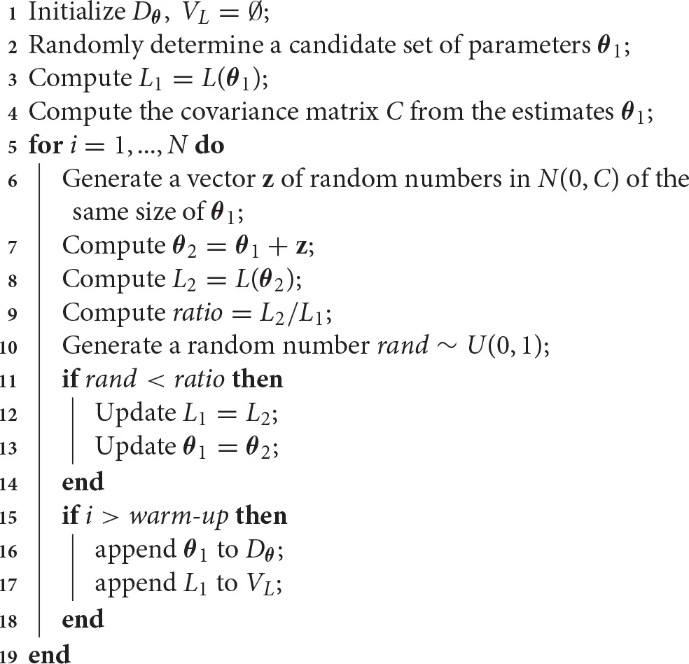 |
Random walk Markov chain Monte Carlo method for parameter estimation.
The algorithm continues generating a new set of parameters by perturbing the previous one through random normally distributed coefficients (Algorithm 2, line 7). This is why the procedure is called random walk MCMC method. In other cases, such as the independent Metropolis-Hastings algorithm, the new set of parameters is proposed independently from the previous [65]. We refer to Brooks et al. [15] for a detailed description of these and other methods. When the new set of parameters is generated, its likelihood is computed (Algorithm 2, line 8) and compared with the previous. If the new likelihood is bigger then the previous (L2/L1 > 1), the new set of parameters is always accepted, otherwise with probability L2/L1 (Algorithm 2, lines 10–13). In order to escape local minima, the latter rule allows the method to randomly accept values that are not better in terms of likelihood. In the long run, the method will return back to the previous value if it was the global solution, otherwise it continues the exploration of the space of parameters. This strategy is in contrast with least squares methods. In those methods, the direction that decreases the objective function is always chosen and, consequently, their results are in general local [66, 67]. Thus, the need to apply a multi-start approach to search for the global solution.
Finally, if the warm-up time is over, the parameters and the likelihood function are stored (Algorithm 2, lines 15–18). This set of parameters is needed to build the a posteriori distributions of parameter estimates, whereas the likelihood values permit to determine the best set in terms of likelihood, if needed. Once these probabilities are estimated, they may provide valuable information, such as the standard deviations or other uncertainty measures, as well as the correlations between the parameters. Moreover, collecting the output of the model along with the parameters provides information about the uncertainty of model results.
As mentioned, MCMC methods can be provided with a priori knowledge on the parameters, such as bounds, experimental standard deviations or distributions of the parameters. When these values are known, the methods can take advantage of them to determine the candidate sets of parameters. In many cases, this information is processed using Bayesian inference [55]. For particularly complex models, exploiting this information may significantly improve the speed of convergence of the algorithm. For the same end, adaptive implementations have been proposed [64]. These implementations generally use statistics from the results, for example the rate at which new candidates are accepted, to properly update the way in which new candidates are proposed [68]. In addition, ad hoc implementations for complex problems have been proposed. In these implementations, multiple independent runs of the algorithm are generated, each of them working on an independent subset of the model or starting from different initial points. The results of these runs are then combined at the end [69, 70]. Despite the use of MCMC methods in discrete problems has been for long time overlooked, some implementations have recently extended their realm to address the problem of inferring discrete and mixed-integer parameters [64, 71].
An optimization method based on Markov chains has drawbacks and advantages. On the one hand, it allows memory-efficient implementations and this is particularly convenient when very complex models are involved. In fact, the algorithm requires only the information about the previous iteration (Algorithm 2, lines 7 and 9), whereas the overall results can be stored at specific sampling rates. On the other hand, the method iterations cannot be computed in parallel, since they depend on the previous. MCMC methods for parameter estimation are usually efficient in the number of objective function evaluations, computing just one evaluation per iteration. However, the lack of termination criteria forces the use of several iterations to ensure the convergence. Nevertheless, they balance this computational cost by returning the a posteriori distributions of the parameter estimates, and therefore more information than other methods.
4. Genetic algorithms
Genetic algorithms (GAs), firstly introduced by Holland in 1975 [72] and then improved and varied during the following decades [73, 74, 75], are nature inspired heuristic stochastic algorithms. As in nature our genes are encoded in chromosomes as strings of nucleotides, these algorithms encode the space of parameters as strings. GAs use these strings to create populations of candidate solutions that evolve according to the principle of survival of the fittest. In analogy with biology, the objective function of GAs is called fitness function, and the principle of survival of the fittest selects those candidates that are better in terms of objective function. GAs mimic the processes of natural selection (Figure 4A), the genetic exchange between two individuals (Figure 4B), known as crossover or recombination, and the random mutation that take place during the process (Figure 4C). One of the key ideas underlying these stochastic algorithms is that the evolution preserves, even under stochastic choices, those strings (or part of them) that guide the process toward the best solution. This concept is formalized in the building block hypothesis and it is detailed in Goldberg [73].
Figure 4
GAs have empirically demonstrated their efficacy and reliability in a variety of fields and for various applications [74]. For example, they have been applied in synthetic and systems biology to determine biomarkers [7, 8], design gene regulatory networks [76], and to estimate parameters [77]. In addition, the convergence of certain GAs has been formally proved for problems involving only discrete parameters [17, 18], and some steps in providing bounds for the runtime have been done [78, 79]. However, GAs lack the formal proof of convergence for problems involving continuous parameters and theoretically proved termination criteria.
As a consequence, the convergence of the algorithms is evaluated a posteriori, for instance introducing a maximum number of allowed iterations or measuring the changes in the fitness of the population. Nevertheless, in the proximity of the solution, the rate at which the evolution takes place and the fitness increases may slow down. Thus, the maximum number of generations may be encountered before reaching the global solution. In some cases, to get around this limitation and since GAs are very effective in determining the region of the space of parameters where the global solution is located, they have been coupled with other methods. In this way, it is possible to precisely locate the global solution once a GA has selected the proper region of the space of parameters or it has provided promising candidate solutions [80].
In Algorithm 3 we present a basic implementation of a GA, called simple GA algorithm (sGA), as described in Goldberg [73]. This algorithm effectively implements the three fundamental steps of selection, recombination and mutation. The algorithm begins mapping the vectors of parameters into strings. In this way, the parameters and the strings are in one-to-one correspondence and the algorithm can work with the more convenient representation. A detailed description of these transformations is provided in Goldberg [73]. An initial population of candidate solutions is then generated. As for the starting points of the multi-start approach, these candidate solutions may be randomly chosen in the space of parameters, or more elaborated sampling techniques may be applied [35–37]. Once the initial population has been produced, the algorithm enters its main loop. Each iteration of the sGA, also referred as generation, produces a new population of strings. Among the many possible termination criteria [81], here we considered the maximum number of generations (Algorithm 3, line 3).
Algorithm 3
|
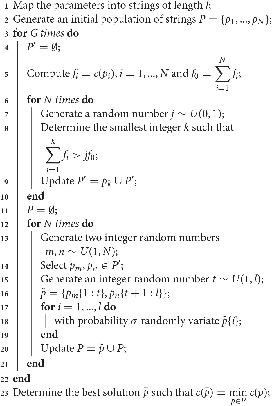 |
A simple Genetic Algorithm.
At each iteration, the selection occurs as a weighted random choice among the candidate solutions, where individuals with higher fitness are more likely to be selected (Algorithm 3, lines 7–8). At this stage, selected individuals are cloned in a new pool of candidates, called intermediate population (Algorithm 3, line 9). The size of the intermediate population, here assumed for simplicity to be equal to the population size N, may vary. The selection of the candidates may occur in many ways [82]. The here-implemented roulette selection [73] divides an interval proportionally to the fitness value of each candidate solution (Algorithm 3, line 5), and then the individuals are randomly selected in this interval (Algorithm 3, lines 7–9). Other popular strategies for the selection of candidate solutions are the genitor algorithm [83] and the tournament selection [84]. The first, generates each newborn as in the roulette selection. However, it does not use an intermediate population and the newborn replaces the worst string in terms of fitness in the original population. On the other hand, the tournament selection randomly picks two or more individuals and only the best in terms of fitness is cloned in the intermediate population.
Once the intermediate population has been determined, its individuals are mated and their genetic material is recombined to determine the next generation of solution candidates. For instance, in the here described single point crossover (Figure 4B), two parents are randomly selected (Algorithm 3, lines 13–14) and at a random position in the string, their genetic material is recombined (Algorithm 3, lines 15–16). As for the selection, the recombination of candidate solutions may be computed in several ways. Some implementations consider more than two parents at time or more points for the crossover, whereas others produce more than one child from the selected parents [16]. In contrast, some implementations determine part of the new population by cloning the best candidates in terms of fitness without recombination at all [85]. This is the case of the elitist selection, which is commonly adopted to enhance the performance of genetic algorithms. When this kind of selection is employed, the convergence to a global solution has been proved for problems involving discrete parameters [17, 18].
After the recombination, the mutation takes place (Figure 4C). With a certain probability σ, usually smaller than 0.01, each element of the string may be randomly replaced (Algorithm 3, line 18) [82] and this new string joins the new population (Algorithm 3, line 20). Once the termination conditions are met, the algorithm determines the best solution among the latest population and returns the corresponding vector of parameters (Algorithm 3, line 23). As for MCMC methods, if the results are not satisfying and the latest population has been saved, the algorithm may be restarted from there in the seek of a better solution.
GAs are powerful approaches to explore high-dimensional spaces of parameters. However, the choice of the population size is crucial: with small populations the algorithms are fast, but they may prematurely converge to local solutions. Larger populations permit the algorithms to better explore the spaces of parameters, but more fitness function evaluations are required. The bigger is the population size, the slower becomes the procedure. In the seek of a balance between the population size and the exploration effectiveness, different implementations of the GAs have been proposed to circumvent the slow down due to large populations. Several of them parallelize the algorithm, or part of it, to speedup the procedure. For example, the master slave parallelization performs the steps of fitness function evaluation, recombination and mutation in parallel, calculating these operations in different cpu cores for different parts of the population [86]. On the other hand, the island model considers many small sub-populations that evolve independently, i.e., islands, and only after a certain number of generations some of their individuals can migrate in other islands [87]. Analogously, the cellular genetic algorithm arranges the candidate strings in a grid of cells and they can mate only with their neighbors [82]. The island and cellular approaches refine many local solutions that are then compared through the migration, which guides the procedure toward the global solution. Moreover, they are suitable for parallel implementation as well, assigning each island or cell to a different cpu core.
GAs are a specific family of algorithms belonging to the class of Evolution Strategy (ES) [88]. This class of optimization techniques shares with the GAs the fundamental steps of selection, recombination, and mutation. In addition, ESs may include steps of self-adaptation, which tune parameters such as the mutation rate [89, 90]. Analogously, ESs may implement more sophisticated selection strategies that increase the selection pressure [88]. For example, the so called plus strategy that may lead to better performance [91]. Certain implementation of GAs take advantages of those improvements as well.
Despite the lack of termination criteria or proven convergence for the most general case, genetic algorithms are considered valuable tools to explore the space of parameters thanks to their flexibility [67]. The continuous exchange of genetic material among individuals permits the algorithm to move in the space of parameters evolving toward the best solution, even if there are many local solutions. Moreover, mutation adds variability to the population. This allows the exploration of new areas of the space of parameters that would otherwise remain unexplored [73]. Finally, GAs can be applied to a broad range of problems, from unconstrained to constrained optimization. They permit to solve problems involving both continuous and discrete variables, as well as problems with continuous or non-continuous objective functions.
5. Conclusions
We presented three powerful methods for global optimization suitable for computational systems biology applications. We highlighted pros and cons of the examined approaches and we provided references for their improvements that may better suit specific tasks.
We presented the multi-start approach for a non-linear least squares method [14] that is suitable for parameter estimation when deterministic simulations are involved, as well as for statistical regression. The least squares methods have many attractive properties like the assured local convergence under specific hypotheses or the valuable termination criteria that assess the convergence of the method. The multi-start approach repeats the least squares procedure from different starting points to explore the space of parameters in the seek of the global solution. However, these methods cannot be applied in case of non-continuous objective functions or discrete parameters. We also illustrated the random walk Markov chain Monte Carlo method [15] that may be applied for many statistical inferences, including parameter estimation, and it is suitable for the framework of Bayesian inference. This method may be applied in case of continuous and non-continuous objective functions, as well as when stochastic simulations are involved. Moreover, its asymptotic convergence to the global solution is assured under mild hypotheses. In spite of this, the asymptotic convergence does not provide any termination criteria, and hence, the convergence cannot be certified. Finally, we have illustrated a simple Genetic Algorithm [74], a heuristic nature-inspired method that can be applied to a broad range of problems. Simple Genetic Algorithm is suitable for problems involving continuous and non-continuous objective functions, as well as continuous and discrete parameters. However, there are no guarantees on its convergence for the most general case, so it requires cautious evaluations of the results.
We focused on the general ideas behind each method, without blurring the description with many details. For this reason, we included simple implementations that, in our opinion, could better guide in understanding the algorithms and the approaches. Therefore, our description does not present all the latest improvements and extensions of the considered optimization techniques. These improvements include more accurate versions of least squares procedures [14] and genetic algorithms [75], implementations of MCMC methods that support discrete variables [71] and hybrid methods that merge MCMC and genetic algorithms [92]. These and many other improvements have enlarged the domain of application of these methods and have ameliorated their accuracy and convergence, leading, however, to more complex procedures.
The presented approaches coexist with a vast literature of exact and heuristics methods. For example, there exist the simplex [9] and the gradient [14] methods, evolutionary strategies [88], the branch and bound [93], the particle swarm [94] or the simulated annealing [95], and countless other approaches. For the sake of simplicity and shortness, we have not covered the entire spectrum of existing deterministic and stochastic methods. We acknowledge that other reviews have already pointed out the importance of global optimization in computational systems biology [5, 67, 96–99]. However, for most of them, the authors efforts were focused on one particular methodology. On the contrary, this review aims at providing a guide to solve common problems in the field, without focusing on one specific approach.
Funding
This work was partially supported by the PAT project S503/2015/664730 Zoomer.
Conflict of interest statement
The authors declare that the research was conducted in the absence of any commercial or financial relationships that could be construed as a potential conflict of interest.
Statements
Author contributions
FR reviewed the introduced optimization algorithms while CP and LM provided conceptual advice. FR and LM contributed to the writing of the manuscript.
Conflict of interest
The authors declare that the research was conducted in the absence of any commercial or financial relationships that could be construed as a potential conflict of interest.
References
1.
WeiseT. Global Optimization Algorithms – Theory and Application. Germany (2009). Available online at: www.it-weise.de
2.
PriamiC. Algorithmic systems biology. Commun ACM (2009) 52:80. 10.1145/1506409.1506427
3.
PriamiCMorineMJ. Analysis of Biological Systems. London: Imperial College Press (2015).
4.
GoryaninI. Computational optimization and biological evolution. Biochem Soc Trans. (2010) 38:1206–9. 10.1042/BST0381206
5.
BangaJR. Optimization in computational systems biology. BMC Syst Biol. (2008) 2:47. 10.1186/1752-0509-2-47
6.
RomeijnHESchoenF. Handbook of Global Optimization, vol. 62. Boston, MA: Springer US (2002).
7.
LacroixSLauriaMScott-BoyerMPMarchettiLPriamiCCaberlottoL. Systems biology approaches to study the effects of caloric restriction and polyphenols on aging processes. Genes Nutr. (2015) 10:58. 10.1007/s12263-015-0508-9
8.
CaberlottoLMarchettiLLauriaMScottiMParoloS. Integration of transcriptomic and genomic data suggests candidate mechanisms for APOE4-mediated pathogenic action in Alzheimer's disease. Sci Rep. (2016) 6:32583. 10.1038/srep32583
9.
PapadimitriouCSteiglitzK. Combinatorial Optimization: Algorithms and Complexity, Unabridged Edn. Mineola, NY: Dover Publications (1998).
10.
MarchettiLRealiFDaurizMBranganiCBoselliLCeradiniGet al. A novel insulin/glucose model after a mixed-meal test in patients with type 1 diabetes on insulin pump therapy. Sci Rep. (2016) 6:36029. 10.1038/srep36029
11.
BoydSVandenbergheL. Convex Optimization. New York, NY: Cambridge University Press (2004).
12.
JamilMYangXS. A literature survey of benchmark functions for global optimization problems citation details: Momin Jamil and Xin-She Yang, a literature survey of benchmark functions for global optimization problems. Int J Math Model Numer Optim. (2013) 4:150–94. 10.1504/IJMMNO.2013.055204
13.
WolpertDHMacreadyWG. No free lunch theorems for optimization. IEEE Trans Evol Comput. (1997) 1:67–82. 10.1109/4235.585893
14.
NocedalJWrightS. Numerical Optimization. Springer Series in Operations Research and Financial Engineering. New York, NY: Springer (2006).
15.
BrooksSGelmanAJonesGMengXL (eds.). Handbook of Markov Chain Monte Carlo, Chapman & Hall/CRC Handbooks of Modern Statistical Methods, vol. 20116022. Boca Raton, FL: Chapman and Hall/CRC (2011).
16.
DavisL. Handbook of Genetic Algorithms. New York, NY: Van Nostrand Reinhold (1991).
17.
RudolphG. Convergence analysis of canonical genetic algorithms. IEEE Trans Neural Netw. (1994) 5:96–101. 10.1109/72.265964
18.
BhandariDMurtyCAPalSK. Genetic algorithm with elitist model and its convergence. Int J Patt Recogn Artif Intell. (1996) 10:731–47. 10.1142/S0218001496000438
19.
RizMPedersenMG. Mathematical modeling of interacting glucose-sensing mechanisms and electrical activity underlying Glucagon-like peptide 1 secretion. PLoS Comput. Biol. (2015) 11:e1004600. 10.1371/journal.pcbi.1004600
20.
MancaVMarchettiLPagliariniR. MP modelling of glucose-insulin interactions in the intravenous glucose tolerance test. Int J Nat Comput Res. (2011) 2:13–24. 10.4018/jncr.2011070102
21.
RealiFMorineMJKahramanoğullarıORaichurSSchneiderHCCrowtherDet al. Mechanistic interplay between ceramide and insulin resistance. Sci Rep. (2017) 7:41231. 10.1038/srep41231
22.
CapuaniFConteAArgenzioEMarchettiLPriamiCPoloSet al. Quantitative analysis reveals how EGFR activation and downregulation are coupled in normal but not in cancer cells. Nat Commun. (2015) 6:7999. 10.1038/ncomms8999
23.
Bollig-FischerAMarchettiLMitreaCWuJKrugerAMancaVet al. Modeling time-dependent transcription effects of HER2 oncogene and discovery of a role for E2F2 in breast cancer cell-matrix adhesion. Bioinformatics (2014) 30:3036–43. 10.1093/bioinformatics/btu400
24.
GuptaSMauryaMRMerrillAHGlassCKSubramaniamS. Integration of lipidomics and transcriptomics data towards a systems biology model of sphingolipid metabolism. BMC Syst Biol. (2011) 5:26. 10.1186/1752-0509-5-26
25.
HermanGABergmanAStevensCKoteyPYiBZhaoPet al. Effect of single oral doses of sitagliptin, a dipeptidyl peptidase-4 inhibitor, on incretin and plasma glucose levels after an oral glucose tolerance test in patients with type 2 diabetes. J. Clin. Endocrinol. Metab. (2006) 91:4612–9. 10.1210/jc.2006-1009
26.
GeLYeSYShanSTZhuZWanHFanS. The model of PK/PD for Danhong injection analyzed by least square method. In: 2015 7th International Conference on Information Technology in Medicine and Education (ITME) (Huangshan: IEEE) (2015). pp. 292–96.
27.
AltmanNKrzywinskiM. Points of significance: simple linear regression. Nat Methods (2015) 12:999–1000. 10.1038/nmeth.3627
28.
MancaVMarchettiL. Log-Gain stoichiometric stepwise regression for MP systems. Int J Found Comput Sci. (2011) 22:97–106. 10.1142/S0129054111007861
29.
MancaVMarchettiL. Solving dynamical inverse problems by means of Metabolic P systems. Biosystems (2012) 109:78–86. 10.1016/j.biosystems.2011.12.006
30.
MancaVMarchettiL. An algebraic formulation of inverse problems in MP dynamics. Int J Comput Math. (2013) 90:845–56. 10.1080/00207160.2012.735362
31.
MarchettiLMancaV. Recurrent solutions to dynamics inverse problems: a validation of MP regression. J Appl Comput Math. (2014) 3:1–8. 10.4172/2168-9679.1000176
32.
MarchettiLMancaV. MpTheory java library: a multi-platform Java library for systems biology based on the Metabolic P theory. Bioinformatics (2015) 31:1328–30. 10.1093/bioinformatics/btu814
33.
BjörckÅ. Numerical Methods for Least Squares Problems. Philadelphia, PA: Society for Industrial and Applied Mathematics (1996).
34.
DennisJESchnabelRB. Numerical Methods for Unconstrained Optimization and Nonlinear Equations, vol. 16. Philadelphia, PA: Society for Industrial and Applied Mathematics (1996).
35.
MorrisMDMitchellTJ. Exploratory designs for computational experiments. J Stat Plan Infer. (1995) 43:381–402. 10.1016/0378-3758(94)00035-T
36.
PronzatoLMüllerWG. Design of computer experiments: space filling and beyond. Stat Comput. (2012) 22:681–701. 10.1007/s11222-011-9242-3
37.
VianaFAC. Things you wanted to know about the latin hypercube design and were afraid to ask. In: 10th World Congress on Structural and Multidisciplinary Optimization. Orlando, FL (2013). pp. 1–9.
38.
KelleyCT. Iterative Methods for Optimization. Philadelphia, PA: Society for Industrial and Applied Mathematics (1999).
39.
GillPEMurrayW. Algorithms for the solution of the nonlinear least-squares problem. SIAM J Numer Anal. (1978) 15:977–92. 10.1137/0715063
40.
LevenbergK. A method for the solution of certain non-linear problems in least squares. Q J Appl Math. (1944) 2:164–8. 10.1090/qam/10666
41.
MarquardtDW. An algorithm for least-squares estimation of nonlinear parameters. J Soc Indust Appl Math. (1963) 11:431–41. 10.1137/0111030
42.
ByrdRHSchnabelRBShultzGA. A trust region algorithm for nonlinearly constrained optimization. SIAM J Numer Anal. (1987) 24:1152–70. 10.1137/0724076
43.
YuanYX. A review of trust region algorithms for optimization. Iciam (2000) 99:271–82.
44.
GeyerC. Practical Markov chain Monte Carlo. Stat Sci. (1992) 7:473–83. 10.1214/ss/1177011137
45.
GamermanDLopesHF. Markov Chain Monte Carlo: Stochastic Simulation for Bayesian Inference, 2nd Edn. Boca Raton, FL: Chapman & Hall/CRC Texts in Statistical Science. Taylor & Francis (2006).
46.
KahramanoğullarıOLynchJF. Stochastic flux analysis of chemical reaction networks. BMC Syst Biol. (2013) 7:133. 10.1186/1752-0509-7-133
47.
ThanhVHPriamiCZuninoR. Efficient rejection-based simulation of biochemical reactions with stochastic noise and delays. J Chem Phys. (2014) 141:134116. 10.1063/1.4896985
48.
MarchettiLPriamiCThanhVH. HRSSA – Efficient hybrid stochastic simulation for spatially homogeneous biochemical reaction networks. J Comput Phys. (2016) 317:301–7. 10.1016/j.jcp.2016.04.056
49.
PahleJ. Biochemical simulations: stochastic, approximate stochastic and hybrid approaches. Brief Bioinformatics (2008) 10:53–64. 10.1093/bib/bbn050
50.
GolightlyAWilkinsonDJ. Bayesian parameter inference for stochastic biochemical network models using particle Markov chain Monte Carlo. Interf Focus (2011) 1:807–20. 10.1098/rsfs.2011.0047
51.
WilkinsonDJ. Stochastic Modelling for Systems Biology. Boca Raton, FL: CRC Press/Taylor & Francis (2012).
52.
KahramanoğullarıOFantacciniGLeccaPMorpurgoDPriamiC. Algorithmic modeling quantifies the complementary contribution of metabolic inhibitions to gemcitabine efficacy. PLoS ONE (2012) 7:e50176. 10.1371/journal.pone.0050176
53.
NewmanKBucklandSTMorganBKingRBorchersDLColeDet al. Modelling Population Dynamics. Model Formulation, Fitting and Assessment Using State-Space Methods. Methods in Statistical Ecology. New York, NY: Springer New York (2014).
54.
MariniGPolettiPGiacobiniMPuglieseAMerlerSRosàR. The role of climatic and density dependent factors in shaping mosquito population dynamics: the case of culex pipiens in northwestern Italy. PLoS ONE (2016) 11:e0154018. 10.1371/journal.pone.0154018
55.
CauchemezSCarratFViboudCValleronAJBoëllePY. A Bayesian MCMC approach to study transmission of influenza: application to household longitudinal data. Stat Med. (2004) 23:3469–87. 10.1002/sim.1912
56.
DiekmannOHeesterbeekHBrittonT. Mathematical Tools for Understanding Infectious Disease Dynamics. Princeton, NJ: Princeton University Press (2013).
57.
MarzianoVPolettiPGuzzettaGAjelliMManfrediPMerlerS. The impact of demographic changes on the epidemiology of herpes zoster: Spain as a case study. Proc Biol Sci. (2015) 282:20142509. 10.1098/rspb.2014.2509
58.
MerlerSAjelliMFumanelliLGomesMFCPionttiAPRossiLet al. Spatiotemporal spread of the 2014 outbreak of Ebola virus disease in Liberia and the effectiveness of non-pharmaceutical interventions: a computational modelling analysis. Lancet Infect Dis. (2015) 15:204–11. 10.1016/S1473-3099(14)71074-6
59.
GeyerCJ. Markov chain Monte Carlo maximum likelihood. In: Computing Science and Statistics: Proceedings of the 23rd Symposium on the Interface, Seattle, WA (1991). pp. 156–63.
60.
CowlesMKCarlinBP. Markov chain Monte Carlo convergence diagnostics: a comparative review. J Am Stat Assoc. (1996) 91:883–904. 10.1080/01621459.1996.10476956
61.
AndrieuCDeFreitas NDoucetAJordanMI. An introduction to MCMC for machine learning. Mach Learn. (2003) 50:5–43. 10.1023/A:1020281327116
62.
MetropolisNRosenbluthAWRosenbluthMNTellerAHTellerE. Equation of state calculations by fast computing machines. J Chem Phys. (1953) 21:1087. 10.1063/1.1699114
63.
HastingsWK. Monte Carlo sampling methods using Markov chains and their applications. Biometrika (1970) 57:97–109. 10.1093/biomet/57.1.97
64.
AndrieuCThomsJ. A tutorial on adaptive MCMC. Stat Comput. (2008) 18:343–73. 10.1007/s11222-008-9110-y
65.
CorcoranJTweedieR. Perfect sampling from independent Metropolis-Hastings chains. J Stat Plan Infer. (2002) 104:297–314. 10.1016/S0378-3758(01)00243-9
66.
MendesPKellDB. Non-linear optimization of biochemical pathways: applications to metabolic engineering and parameter estimation. Bioinformatics (1998) 14:869–83. 10.1093/bioinformatics/14.10.869
67.
MolesCGMendesPBangaJR. Parameter estimation in biochemical pathways: a comparison of global optimization methods. Genome Res. (2003) 13:2467–74. 10.1101/gr.1262503
68.
AtchadeYFRosenthalJS. On adaptive Markov chain Monte Carlo algorithms. Bernoulli (2005) 11:815–28. 10.3150/bj/1130077595
69.
NeiswangerWWangCXingE. Asymptotically exact, embarrassingly parallel MCMC. CoRR abs/1510.0 (2015).
70.
AndrieuCDoucetAHolensteinR. Particle Markov chain Monte Carlo methods. J R Stat Soc Ser B Stat Methodol. (2010) 72:269–342. 10.1111/j.1467-9868.2009.00736.x
71.
VrugtJATerBraak CJF. DREAM(D): an adaptive Markov Chain Monte Carlo simulation algorithm to solve discrete, noncontinuous, and combinatorial posterior parameter estimation problems. Hydrol Earth Syst Sci. (2011) 15:3701–13. 10.5194/hess-15-3701-2011
72.
HollandJH. Adaptation in Natural and Artificial Systems: An Introductory Analysis with Applications to Biology, Control and Artificial Intelligence. Cambridge, MA: MIT Press (1992).
73.
GoldbergDE. Genetic Algorithms in Search, Optimization, and Machine Learning. Boston, MA: Addison-Wesley Longman Publishing Co. Inc. (1989).
74.
MitchellM. An Introduction to Genetic Algorithms. Cambridge, MA: MIT Press (1998).
75.
SivanandamSNDeepaSN. Introduction to Genetic Algorithms, 1st Edn. Berlin; Heidelberg: Springer Publishing Company, Incorporated (2007).
76.
ChuD. Evolving genetic regulatory networks for systems biology. In: 2007 IEEE Congress on Evolutionary Computation (Singapore: IEEE) (2007). pp. 875–82.
77.
CartaAChavesMGouzéJL. A simple model to control growth rate of synthetic E. coli during the exponential phase: model analysis and parameter estimation. In: GilbertDHeinerM editors. Computational Methods in Systems Biology. Lecture Notes in Computer Science.Berlin; Heidelberg: Springer (2012).
78.
OlivetoPSWittC. On the analysis of the simple genetic algorithm. In: Proceedings of the Fourteenth International Conference on Genetic and Evolutionary Computation Conference - GECCO '12. New York, NY: ACM Press (2012). p. 1341.
79.
OlivetoPSWittC. Improved time complexity analysis of the simple genetic algorithm. Theor Comput Sci. (2015) 605:21–41. 10.1016/j.tcs.2015.01.002
80.
GoldbergDEVoessnerS. Optimizing global-local search hybrids. In: Proceedings of the Genetic and Evolutionary Computation Conference, vol. 1Orlando, FL (1999). pp. 220–8.
81.
SafeMCarballidoJPonzoniIBrignoleN. On stopping criteria for genetic algorithms. In: Advances in Artificial Intelligence – SBIA 2004. Berlin; Heidelberg: Springer (2004). pp. 405–13.
82.
WhitleyD. A genetic algorithm tutorial. Stat Comput. (1994) 4:65–85. 10.1007/BF00175354
83.
WhitleyLD. The GENITOR Algorithm and selection pressure: why rank-based allocation of reproductive trials is best. In: ICGA, vol. 89. Fairfax, VA (1989). pp. 116–23.
84.
MillerBLGoldbergDE. Genetic algorithms, tournament selection, and the effects of noise. Comp Syst. (1995) 9:193–212.
85.
BalujaSCaruanaR. Removing the genetics from the standard genetic algorithm. In: ICML (1995). pp. 1–11.
86.
Cantú-PazE. A survey of parallel genetic algorithms. Calcul Paralleles Reseaux Syst Repart. (1998) 10:141–71.
87.
WhitleyDRanaSHeckendornRB. The island model genetic algorithm: on separability, population size and convergence. J Comput Inform Technol. (1999) 7:33–47.
88.
BeyerHGSchwefelHP. Evolution strategies – A comprehensive introduction. Nat Comput. (2002) 1:3–52. 10.1023/A:1015059928466
89.
OstermeierAGawelczykAHansenN. Step-size adaptation based on non-local use of selection information. In: DavidorYSchwefelHPMännerR. editors. Parallel Problem Solving from Nature — PPSN III. PPSN 1994. Lecture Notes in Computer Science, Berlin; Heidelberg: Springer (1994).
90.
HansenN. The CMA evolution strategy: a tutorial. arXiv:1604.00772 (2016).
91.
JagerskupperJStorchT. When the plus strategy outperforms the comma-when not. In: 2007 IEEE Symposium on Foundations of Computational Intelligence (Tahoe City, CA: IEEE) (2007). pp. 25–32.
92.
BraakCJFT. A Markov chain Monte Carlo version of the genetic algorithm differential evolution: easy Bayesian computing for real parameter spaces. Stat Comput. (2006) 16:239–49. 10.1007/s11222-006-8769-1
93.
DerhyMF (ed.). Integer programming: the branch and bound method. In: Linear Programming, Sensitivity Analysis & Related Topics, Upper Saddle River, NJ: Prentice Hall (2010).
94.
KennedyJEberhartR. Particle swarm optimization. In: Proceedings of ICNN'95 - International Conference on Neural Networks, vol. 4. (Honolulu, HI: IEEE) (1995). pp. 1942–8.
95.
KirpatrickSGelattCDVecchiMP. Optimization by simulated annealing. Science (1983) 220:671–80. 10.1126/science.220.4598.671
96.
WilkinsonDJ. Bayesian methods in bioinformatics and computational systems biology. Brief Bioinformatics (2007) 8:109–16. 10.1093/bib/bbm007
97.
LillacciGKhammashM. Parameter estimation and model selection in computational biology. PLoS Comput Biol. (2010) 6:e1000696. 10.1371/journal.pcbi.1000696
98.
WangYZhangXSChenL. Optimization meets systems biology. BMC Syst Biol. (2010) 4:S1. 10.1186/1752-0509-4-S2-S1
99.
Balsa-CantoEBangaJREgeaJAFernandez-VillaverdeADeHijas-Liste GM. Global optimization in systems biology: stochastic methods and their applications. Adv Exp Med Biol. (2012) 736:409–24. 10.1007/978-1-4419-7210-1_24
Summary
Keywords
optimization, least squares algorithms, Markov chain Monte Carlo, genetic algorithms, computational systems biology, parameter estimation, global optimization, mathematical modeling
Citation
Reali F, Priami C and Marchetti L (2017) Optimization Algorithms for Computational Systems Biology. Front. Appl. Math. Stat. 3:6. doi: 10.3389/fams.2017.00006
Received
30 November 2016
Accepted
24 March 2017
Published
11 April 2017
Volume
3 - 2017
Edited by
Vittorio Romano, University of Catania, Italy
Reviewed by
Carola Doerr, CNRS and Pierre et Marie Curie University, France; Vincenzo Bonnici, University of Verona, Italy
Updates
Copyright
© 2017 Reali, Priami and Marchetti.
This is an open-access article distributed under the terms of the Creative Commons Attribution License (CC BY). The use, distribution or reproduction in other forums is permitted, provided the original author(s) or licensor are credited and that the original publication in this journal is cited, in accordance with accepted academic practice. No use, distribution or reproduction is permitted which does not comply with these terms.
*Correspondence: Luca Marchetti marchetti@cosbi.eu
This article was submitted to Optimization, a section of the journal Frontiers in Applied Mathematics and Statistics
Disclaimer
All claims expressed in this article are solely those of the authors and do not necessarily represent those of their affiliated organizations, or those of the publisher, the editors and the reviewers. Any product that may be evaluated in this article or claim that may be made by its manufacturer is not guaranteed or endorsed by the publisher.