Finite Sample Corrections for Parameters Estimation and Significance Testing

1. Introduction

The current era of Big Data has ushered in a new way to look at Science—and that is letting the data speak for itself. Because of this, we are now much more concerned about empirical distributions than we have in the past, and to check what the empirical distributions could be in statistically rigorous ways. In the past, many tests on empirical data were performed against the univariate normal distribution [1]. Some of these tests focus on the goodness-of-fit of higher order moments [2–4], while others compare the test statistics against an Empirical Distribution Function (EDF) [5–8]. In 2011, Nornadiah and Yap performed a systematic comparison of Anderson-Darling (AD), Lilliefors, Kolmogorov-Smirnov (KS), and Shapiro-Wilk (SW), using numerical simulations and concluded that the SW test is the best, followed closely by the AD test for a given significance [9].

Among these tests, the KS and Lilliefors tests can also be applied to non-normal distributions. In fact, many real-world data do not follow normal distributions. For instance, many social systems are known to have power-law distributions [10]. These include the financial returns [11–14], word count [15, 16], city size [17, 18], home price [19–21], wealth and income [22, 23] distributions. One simple but naive way to detect a power law is to plot the data in log-log scale, fit it to a straight line and determine the goodness of fit. However, this simple method has three major flaws: (i) many distributions (e.g., exponential, gamma, log-normal) can also look straight in log-log plot, especially if the range of data is small; (ii) the goodness of fit only quantifies how well the fit is visually but does not tell us how plausible the fit is; and (iii) if our data looks straight in both log-log and semi-log plots, the goodness of fit values obtained from the two cannot be directly compared since they were obtained from plots of different scales. Clauset, Shalizi, and Newman (CSN) address precisely these three points in their 2009 paper [24], and the test they proposed is now considered by many the gold standard in curve fitting. We shall describe the main idea of the CSN technique in greater mathematical detail in section 2.

Since the CSN test can be applied across distributions, we also use it to fit data that appear exponentially distributed. On many occasions, we discovered that the exponential fits look good visually, but have significance values (p-value) much lower than fits of other data to power laws, even though the latter look visibly poorer. In fact, in the CSN paper where empirical data is tested against a power law (PL), log-normal, exponential (EXP), stretched exponential, and a power law with cut-off, the exponential distribution consistently performs poorer than the other distributions. This was also the case when Brzezinski tested the upper-tail wealth data for China, Russia, US, and the World using the CSN method [25]. In these papers, the data might truly be non-exponentially distributed, so it is not surprising the exponential fits fail. However, the low p-values for the visually convincing exponential fits to our data suggest that something fundamental was missed.

We realized there are two issues associated with fitting data to distributions defined over (0, ∞). First, there is the finite largest element effect (FLE), due to the largest element in the data being finite. Second, we also encounter the finite number of elements effect (FNE), due to the sample size dependence of the goodness-of-fit measures. These two finite sample effects are well studied for Generalized Moment Methods (GMMs) [26, 27] but often neglected in tests of statistical significance. After describing the CSN test, we illustrate in section 2 the FLE and FNE effects by applying the test to three real data sets. With the insights gained, we designed both the estimators and test statistic to account for the FLE and FNE effects in section 3.1. Since real data is frequently polluted by noise, we also discuss the impact of noise on the p-value, and propose a test statistic that accounts for noise in section 4. Finally, in section 5, we apply the adjusted test statistics on our real data sets and compare the p-values obtained against those from the CSN test.

2. Reexamining Significance Testing for Empirical Distributions

Sometimes we have reasons to believe that our large data sets may be described by well known distributions, such as the normal distribution, power law distribution, exponential distribution, and so on, but with best-fit parameter values that we need to determine. Commonly used methods to perform parameter estimation include Maximum Likelihood Estimation (MLE) [28], Maximum Entropy Method (MEM) [29–31], least square regressions [32], and direct or indirect computation of moments [33]. Since it is possible to fit any distribution to any data set, we need to compute its goodness of fit, which can be the KS distance [7], the coefficient of determination (R²) and other forms of distance measure [34, 35].

In a recent statement, the American Statistical Association warned the scientific community that the p-value “was never intended to be a substitute for scientific reasoning” [36, para. 2], and outline six principles that can prevent its misuse [37]. A Nature commentary on this statement also added that “[r]esearchers should describe not only the data analyses that produced statistically significant results, …, but all statistical tests and choices made in calculations” [38, para. 3]. We heed the warning in this paper, but argue that when properly computed and interpreted, the p-value is useful in that it provides a quantitative and objective alternative to visual inspection of the fits. The latter is frequently subjective and biased. This utility becomes important when we are comparing fits of two or more data sets to two or more distributions, and have the ambiguity of being able to choose from two or more definitions of goodness of fit. This is why we need to go beyond the goodness of fits, to establish how plausible different distributions are for different data sets.

In 2009, Clauset, Shalizi, and Newman (CSN) did precisely this by coming up with a p-test model that use the well-known PL distribution as an illustration. They started by writing down the probability density function for the PL distribution

$\begin{array}{cc}{f}_{PL}=\frac{\alpha -1}{x_{min}^{1-\alpha }}{x}^{-\alpha },& (1)\end{array}$

for x ∈ [x_min, ∞), with exponent α. The CSN p-test involves four major steps:

CSN(i) MLE Estimation of α: Given an empirical data with S observations, with the ordered statistic Y = {y₁, y₂, …, y_S}, sorted such that y_i ≤ y_i+1, the CSN algorithm (CSN(ia)) first constructs the S subsets ${\text{X}}^{(j)}=\left\{x_1^{(j)}=y_j,x_2^{(j)}=y_{j+1},\dots ,x_{N=S-j+1}^{(j)}=y_S\right\}$. (CSN(ib)) For each X^(j), we estimate α^(j) using the MLE method that maximizes the log-likelihood function,

$\begin{array}{cc}\ln {\mathbb{L}}_{PL}=\ln \left[{\displaystyle \prod _{i=1}^N{f}_{PL}}\left(x_i|\widehat{\alpha }\right)\right]=N\ln \left(\frac{\widehat{\alpha }-1}{x_{min}}\right)-\widehat{\alpha }{\displaystyle \sum _{i=1}^N\ln \left(\frac{x_i}{x_{min}}\right)}.& (2)\end{array}$

Applying the maximizing condition $\frac{\partial (\ln \mathbb{L})}{\partial \alpha }=0$ yields

$\begin{array}{cc}\widehat{\alpha }=1+{\langle \ln \frac{x}{x_{min}}\rangle }^{-1},& (3)\end{array}$

where the hat indicates an estimated parameter and $\langle x\rangle =\frac{1}{N}\sum _{i=1}^N{x}_i$ indicates the expectation value of the random variable x.

CSN(ii) KS Distance: If X follows probability distribution function f_X with cumulative distribution function F_X, then its probability integral transform u = F_X(x) is a standard uniform distribution function (U(0, 1)). For any PL distributed sample X = {x₁ = x_min, x₂, …, x_N} with estimated $\widehat{\alpha }$, we (CSN(iia)) first transform the sample to $U^{(s)}={\left\{u_i^{(s)}=F_{PL}(x_i|\widehat{\alpha })\right\}}_{i=1}^N$. (CSN(iib)) Then we calculate the KS distance

$\begin{array}{cc}{d}_{KS}={\forall }_{i=1}^N\sup \left(\left|u_i-\frac{i}{N}\right|\right)& (4)\end{array}$

between U^(s) and U(0, 1). Here we make use of the fact that the CDF of U(0, 1) is a linear function, F_U(u) = u.

CSN(iii) Determining x_min: To determine x_min, (CSN(iiia)) we calculate the KS distance for each X^(j) with its corresponding ${\widehat{\alpha }}^{(j)}$. (CSN(iiib)) The set X^(j) that yields the lowest KS distance ($d_{KS}^{(em)}$) gives us ${\widehat{x}}_{min}^{(em)}=y_j$ and ${\widehat{\alpha }}^{(em)}={\widehat{\alpha }}^{(j)}$. The superscript “(em)” indicates a parameter obtained from empirical data.

CSN(iv) Significance Testing: After ${\widehat{\alpha }}^{(em)}$ and ${\widehat{x}}_{min}^{(em)}$ have been estimated from Y = {y₁, y₂, …, y_S}, we test how plausible it is for $\text{X}=\left\{x_1={\widehat{x}}_{min}^{(em)},x_2,\dots ,x_N\right\}\subset \text{Y}$ to be a sample taken from a PL distribution. This is done by (CSN(iva)) sampling the PL M times using ${\widehat{\alpha }}^{(em)}$ and ${\widehat{x}}_{min}^{(em)}$. (CSN(ivb)) For the mth simulated sample we go through CSN(i) to CSN(iii) to obtain $d_{KS}^{(m)}$. (CSN(ivc)) The significance measure

$\begin{array}{cc}p=\frac{1}{M}{\displaystyle \sum _{m=1}^M{\mathbb{I}}_{\{d_{KS}^{(em)}<d_{KS}^{(m)}\}}},{\mathbb{I}}_{\left\{x\right\}}=\{\begin{array}{l}1\text{if}x=\text{True};\hfill \\ 0\text{if}x=\text{False}\hfill \end{array}& (5)\end{array}$

is the fraction of simulated samples whose fits are poorer than that of the data.

Extending the CSN method to other distributions, we performed p-testing on the Taiwan home price per square foot (fitted to EXP), Taiwan income (fitted to EXP), and the Straits Times Index normalized return (fitted to PL) (see Supplementary Information section 3 for more descriptions on the data sets). The fits and p-values are shown in Figure 1. All fits are visually good yet only the p-value for the Taiwan housing is appreciable. We realized the reason for this is simple: while the EXP and PL distributions are defined over (0, ∞), when we collect data from the real world we can only obtain a finite number of elements. Moreover, the largest element in the data is finite. However, existing tests for statistical significance generally do not account for the effects produced by having a finite number of elements (FNE) and a finite largest element (FLE). In the next section we will explain how the parameters and test statistics can be adjusted for FNE and FLE.

FIGURE 1

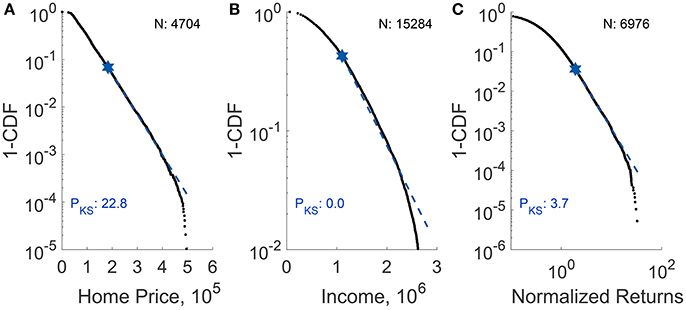
Figure 1. p-testing on (A) 2012–2014 Taiwan home price per square foot, (B) 2012 Taiwan lower-tail income (fitted to EXP), and (C) 2009–2016 Straits Times Index normalized return (fitted to PL). For each plot, N represents the number of data points (larger than x_min) fitted. the black dots represent empirical data while the blue dashed line represents the fit. All fits are visually good, yet only the p-value (P_KS in percentage) for Taiwan home price is appreciable.

At this stage, we might wonder whether the Taiwan income data would have been better fitted to a truncated EXP (TEXP) distribution

$\begin{array}{cc}{f}_{EXP}^{trunc}(x)=\frac{\beta \exp [-\beta (x-x_{min})]}{1-\exp [-\beta (x_{max}-x_{min})]},& (6)\end{array}$

since it is obtained by removing the power-law tail. The Taiwan home price per square foot data was also truncated, but for a different reason: the small number of largest elements are clearly outliers that would not fit the EXP distribution. Ideally, we should be using untruncated data, like the Straits Times Index data, to illustrate the method that we will describe in the following sections. In the rest of the paper, we will use all three data sets as if they were untruncated, to illustrate how well our method works on different data types. To do so, we will compare the adjusted parameter and test statistic against the unadjusted parameter and test statistic meant for the untruncated EXP distribution.

3. Finite-Sample Adjustments

3.1. Parameter Adjustment for Finite Largest Element

Here, we will illustrate the effects of FLE using an asymptotic EXP distribution. The same discussion can be generalized to other distributions (see Supplementary Information section 1).

The EXP distribution is defined as

$\begin{array}{cc}{f}_{EXP}\left(x\right)=\beta \exp \left[-\beta \left(x-x_{min}\right)\right],& (7)\end{array}$

with β as a sole parameter for x ∈ [x_min, ∞). Maximizing the likelihood function $𝕃={\prod }_{i=1}^{N}P(X=x_i|x_{min},\widehat{\beta })$, we find the estimated parameter

$\begin{array}{cc}\widehat{\beta }=\frac{1}{\langle x\rangle -x_{min}}.& (8)\end{array}$

If we use the mean obtained from data 〈x〉_data as 〈x〉 in Equation (8) we will obtain the unadjusted estimator β_unadj. However, due to the FLE, we can only average up till x_max. As such 〈x〉_data will be biased downwards and Equation (8) over-estimates $\widehat{\beta }$.

To adjust for the FLE, we add the truncated part back into 〈x〉_data, to define the adjusted 〈x〉_adj as

$\begin{array}{cc}\begin{array}{l}{\langle x\rangle }_{adj}={\langle x\rangle }_{data}{\displaystyle {\int }_{x_{min}}^{x_{max}}{f}_{EXP}}\left(x\right)dx+{\displaystyle {\int }_{x_{max}}^{\infty }x}{f}_{EXP}\left(x\right)dx.\\ ={\langle x\rangle }_{data}\left\{1-\exp \left[-\beta \left(x_{max}-x_{min}\right)\right]\right\}\\ +\frac{\exp \left[-\beta \left(x_{max}-x_{min}\right)\right]}{\beta }\left[\beta x_{max}+1\right].\end{array}& (9)\end{array}$

Inserting 〈x〉_adj into Equation (8), we obtain a nonlinear equation

$\begin{array}{cc}\begin{array}{l}\left[{\widehat{\beta }}_{adj}\left(x_{max}-{\langle x\rangle }_{data}\right)+1\right]\exp \left[-{\widehat{\beta }}_{adj}\left(x_{max}-x_{min}\right)\right]\\ +{\widehat{\beta }}_{adj}\left({\langle x\rangle }_{data}-x_{min}\right)-1=0\end{array}& (10)\end{array}$

that we solve using MATLAB's builtin nonlinear solver function nlinfit() to obtain ${\widehat{\beta }}_{adj}$.

To test the performance of this adjustment formula, we simulated 1, 000 sets of EXP distributed data for $10^{-4}\le {\beta }_T\le 10^2$, by using the inverse cumulative function for EXP distribution

$\begin{array}{cc}{F}_{EXP}^{-1}(u,{\beta }_T)=x_{min}-\frac{1}{{\beta }_T}\ln (1-u).& (11)\end{array}$

This transforms U(0, 1) distributed elements {u_i} to EXP distributed elements {x_i}. Using this transformation $F_{EXP}^{-1}$, 0 and 1 map to x_min and ∞ respectively. It is also useful to note that Equation (11) is the inverse of the CDF of the EXP distribution,

$\begin{array}{cc}{F}_{EXP}(x,{\beta }_T)=1-\exp \left[\beta \left(x_{min}-x\right)\right].& (12)\end{array}$

To simulate the effect of a FLE with $x_{max}=F_{EXP}^{-1}(0.9)$, we sampled 1,000 sets of EXP distributed data using U(0, 0.9) instead of U(0, 1) with x_min = 0. Thereafter, we estimated ${\widehat{\beta }}_{unadj}$ and ${\widehat{\beta }}_{adj}$ using Equations (8) and (10). Figure 2 shows the relative estimation errors

$\begin{array}{cc}\Delta \widehat{\beta }=\frac{\sqrt{\langle {\left(\widehat{\beta }-{\beta }_T\right)}^2\rangle }}{{\beta }_T}& (13)\end{array}$

of ${\widehat{\beta }}_{unadj}$ and ${\widehat{\beta }}_{adj}$ with respect to the true beta β_T. As we can see from the Figure 2, $\Delta {\widehat{\beta }}_{unadj}$ is about 38% for small samples N ~ 10² and decreases to 34% for large samples N ~ 10⁴. On the other hand, $\Delta {\widehat{\beta }}_{adj}$ starts at 20%, but decreases to 2% as the number of data points is increased. Although it can be shown that the bias of ${\widehat{\beta }}_{unadj}$ vanishes with increasing sample sizes [24, 39], we find it converging very slowly with increasing sample size in the unfortunate situation of a small x_max. In contrast, ${\widehat{\beta }}_{adj}$ converges very quickly even for small x_max as we have accounted for the FLE.

FIGURE 2

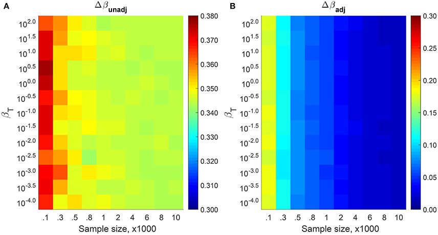
Figure 2. Relative estimation errors of (A) ${\widehat{\beta }}_{unadj}$ and (B) ${\widehat{\beta }}_{adj}$ measured from 1,000 simulated samples using different β_T and N with x_min = 0 and $x_{max}=F_{EXP}^{-1}(0.9)$. Due to the FLE, Δβ_unadj remains high (close to the theoretical relative error of ϵ(δ = 0.1, x_min = 0) = 0.1[1 − ln(0.1)] ≈ 33%) even for large N. In contrast, Δβ_adj decreases rapidly with increasing N.

In the Supplementary Information section 1, we show details for our derivation of the theoretical estimation

$\begin{array}{cc}\begin{array}{l}{\beta }_{unadj}\approx {\beta }_T+{\beta }_T\left[{\beta }_T{x}_{max}+1\right]\exp \left(-{\beta }_T(x_{max}-x_{min})\right)\\ +{O}\left\{{\left({\beta }_T{x}_{max}+1\right)}^2\exp \left(-2{\beta }_T(x_{max}-x_{min})\right)\right\}.\end{array}& (14)\end{array}$

By defining $x_{max}=x_{min}-{\beta }_T^{-1}\ln (\delta )$, and substitute x_max in Equation (14) with δ, the theoretical relative estimation error is expressed as

$\begin{array}{cc}\Delta {\beta }_{unadj}=\delta \left[1-\ln (\delta )+{\beta }_T{x}_{min}\right],\delta \in [0,1].& (15)\end{array}$

Equation (15) shows that the estimation error has no explicit dependence on sample size. This tells us that the ${\widehat{\beta }}_{unadj}$ is always larger than the β_T because of the FLE effect. The convergence rate then depends on how rapidly x_max approaches infinity (δ approaches zero) with increasing sample size.

3.2. Test Statistic Adjustment for FLE

For a finite sample, F_EXP(x) < 1 for all x < ∞. Mathematically, this means that F_EXP(x) ~ U(0, 1 − δ), where $F_{EXP}^{-1}(x_{max})=1-\delta$. This observation is important, because d_KS is obtained by comparing $U^{(s)}={\left\{u_i^{(s)}=F_{EXP}(x_i|\widehat{\beta })\right\}}_{i=1}^N$ against U(0, 1) (see Equation 4). This tell us that for a fair comparison, we need to rescale all elements in U^(s) by a factor of 1/(1−δ). Figure 3 shows the d_KS measured for the 1000 sets of EXP distributed data with finite largest element $x_{max}=F^{-1}(0.9)$ for various β_T and sample sizes N. For each sample, we use Equation (10) to estimate the ${\widehat{\beta }}_{adj}$ and transformed this data to U^(s) using Equation (12). After that, we measure d_KS with Equation (4) to obtain unadjusted KS distance, KS_unadj and adjusted KS distance, KS_adj using the non-rescaled and rescaled U^(s), respectively. KS_unadj goes from 0.14 for small samples N ~ 10², to 0.10 for large samples N ~ 10⁵. In contrast, KS_adj decrease from 0.06 for small samples to 0.006 for large samples.

FIGURE 3

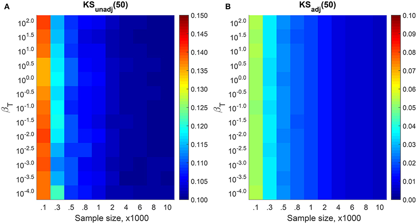
Figure 3. The median KS distances for (A) KS_unadj and (B) KS_adj measured from 1,000 simulated samples using different β_T and N. The x_min is set to 0 and $x_{max}=F_{EXP}^{-1}(0.9)$. Because of the FLE, KS_unadj remains above δ = 0.10 while KS_adj converges to zero for large N.

3.3. Adjustment for Finite Number of Elements

Until now, we have only discussed adjustments to the estimated parameter and the KS distance to eliminate the bias caused by the FLE. Besides the FLE effect, we also need to consider the bias caused by having a finite number of elements in the sample. As we can see from Figure 3, the KS distance decreases as the sample size increases. Therefore, in order to have a fair comparison of the goodness of fit for various sample sizes, we need to determine how d_KS changes as a function of N. To do this, we simulated 10⁶ samples of various sizes N from U(0, 1). For each sample we determined d_KS using Equation (4), so that for each N we end up with 10⁶ KS distances. In Figure 4 we show the KS distances at different deciles, which exhibits the asymptotic behavior

$\begin{array}{cc}{d}_{KS}({\wp }_{KS},N)=\frac{{\left(\frac{100}{{\wp }_{KS}}-1\right)}^{-0.176}\exp (-0.274)}{N^{0.492}},N>50& (16)\end{array}$

that we settled for, after experimenting with several functional forms (see Supplementary Information section 2). This result agrees with our expectation that d_KS → 0 as N → ∞. It also suggests that if we have two samples with sizes N₁ and N₂ from the same distribution, we should compare $N_1^{0.492}{d}_{KS}^{(1)}$ against $N_2^{0.492}{d}_{KS}^{(2)}$. Otherwise, if N₂ > N₁ then naturally $d_{KS}^{(2)}<d_{KS}^{(1)}$ and we will be lead to the wrong conclusion that the N₂ sample fits the distribution better.

FIGURE 4

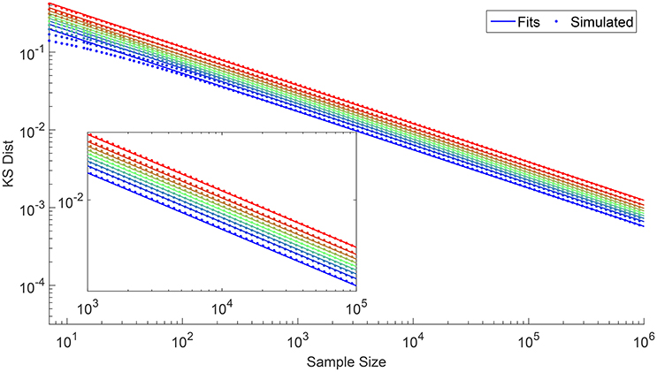
Figure 4. Log-log plot of d_KS against N for different deciles going from the 10th percentile (blue) to the 90th (red), obtained from 10⁶ simulations.

In this section, we presented explicitly the procedures to obtain the adjusted parameter, as well as the steps to perform significance testing on this estimated parameter. Although we demonstrated this explicitly using the EXP distribution as an example, one should note that this method can also be applied to other distributions. The inclusion of x_max when fitting empirical data have been previously considered by [40–42] for the truncated PL distribution. Like these, the method presented in this paper can be easily extended to fit different distributions, but unlike these, we can easily conduct significance testing across them. This is because by extending x_max to infinity, we can compute the probability integral transform to map arbitrary distributions to the standard uniform distribution, and ensure that during statistical significance testing our goodness-of-fit measure can be distribution independent [see CSN(ii)].

More importantly, fitting data to untruncated distributions defined over [x_min, ∞) is commonly encountered in practice, where no x_max is expected from theoretical considerations, but the largest element in our data is finite. If we fit to the truncated versions of the distributions, we might get better estimates of the distribution parameters, but we will not be able to justify inserting these estimates into the untruncated distributions, in the absence of a limiting procedure involving larger and larger x_max. Moreover, when researchers expect to be dealing with the untruncated distribution, they will not use the truncated distribution for estimation. In contrast, our self-consistent adjustment procedure would be ontologically easier to justify.

4. The Effects of Random Noise

Besides having to work with finite samples and finite largest elements, we will also in practice encounter imperfections while collecting samples for various reasons, such as undetected samples, contamination by background noise, and recording errors. We call such noises that occur at the element level elementary noise. When we convert these samples to a distribution, noise will also be present at the distribution level that we refer to as distribution noise. In principle the information at the distribution level is more robust compared to the elementary level, as we expect random and thus uncorrelated noise to cancel each other. This means that the distribution is less sensitive to elementary noise, but we still worry whether the distribution noise may play an important role in our test of statistical significance. In order to account for the effects of distribution noise, we need to first be able to quantify distribution noise, and thereafter understand how it affects significance testing.

Suppose we now randomly generate a set of EXP data. After adjusting for FLE, we obtained the distribution parameters and use it to transform this set to $U^{(s)}={\left\{u_i^{(s)}=F_{EXP}(x_i|\widehat{\beta })\right\}}_{i=1}^N$ following the procedure outlined in section 3.1. Then as illustrated in Figures 5A–C, a natural way to measure the distribution noise is to plot the histogram, count the frequency for each bin, and compare it to the expected frequency from U(0, 1). Since this can be more accurately done for smaller bin sizes, we use the intervals between sorted elements as a collection of non-uniform bins, as shown in Figures 5D–F. For a data set consisting of N elements, each bin carry a weight of 1/N, evenly distributed within the interval (u_i−1, u_i], such that the probability density is

$\begin{array}{cc}f(u_{i-1},u_i)=\frac{\frac{1}{N}}{u_i-u_{i-1}}.& (17)\end{array}$

As the theoretical probability density for U(0, 1) is 1, we define the distribution noise d_DN mathematically to be

$\begin{array}{cc}\begin{array}{l}{d}_{DN}=\sqrt{\frac{{\displaystyle {\sum }_{i=1}^N{\left(u_i-u_{i-1}\right)}^2}{\left[f(u_{i-1},u_i)-1\right]}^2}{{\displaystyle {\sum }_{i=1}^N{\left(u_i-u_{i-1}\right)}^2}}}\\ =\sqrt{\frac{{\displaystyle {\sum }_{i=1}^N{\left(u_i-u_{i-1}\right)}^2}{\left(\frac{1}{N(u_i-u_{i-1})}-1\right)}^2}{{\displaystyle {\sum }_{i=1}^N{\left(u_i-u_{i-1}\right)}^2}}},\end{array}& (18)\end{array}$

where u₀ = 0 and u_N = 1. We need to weigh the deviation of each bin by ${(u_i-u_{i-1})}^2$ because the bins are non-uniform, and also to keep d_DN finite.

FIGURE 5

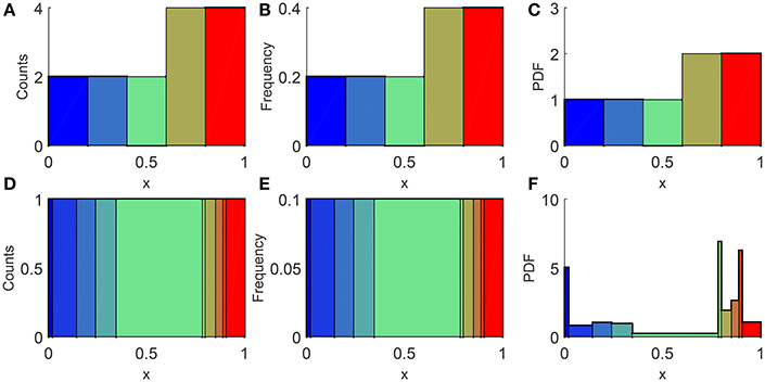
Figure 5. Illustration of the distribution noise we would measure if we sample 10 elements from U(0, 1), rescaled such that the largest element becomes 1. In (A,C) we use 5 uniform bins whereas in (D,F) we use the intervals between sorted elements as the bins. Counts are shown as (A,D), and frequencies are shown as (B,E). Whereas the probability densities calculated using Equation (17) are shown on the as (C,F).

4.1. Relation between Distribution Noise and Sample Size

As with section 3.3, we simulated 10⁶ samples from U(0, 1) with different N. For each sample, we calculate the distribution noise d_DN using Equation (18) and plot its deciles against N as shown in Figure 6. After experimenting with several functional forms, we write down the relationship between d_DN and N at percentile ℘_DN as

$\begin{array}{cc}{d}_{DN}({\wp }_{DN},N)=\langle d_{DN}\rangle +\Phi ({\wp }_{DN}-50)\frac{\exp \left(-\frac{{\left[50-|{\wp }_{DN}-50|\right]}^{0.430}}{|{\wp }_{DN}-50{|}^{0.302}}\right)}{N^{0.495}},& (19)\end{array}$

where Φ(x) represents the sign of x, and

$\begin{array}{cc}\langle d_{DN}\rangle =\sqrt{\frac{1}{2}+\frac{2-N}{2N^2}}\left(\frac{N}{N+0.5}\right)& (20)\end{array}$

is the analytically derived distribution noise, that converges to $1/\sqrt{2}$ as N → ∞ (refer to Supplementary Information section 2 for more details). This result suggests that if we have two samples with sizes N₁ and N₂ with N₂ > N₁ from the same distribution, we should compare $N_1^{0.495}(d_{DN}^{(1)}-1/\sqrt{2})$ against $N_2^{0.495}(d_{DN}^{(2)}-1/\sqrt{2})$. Otherwise, we risk making the wrong conclusion that the N₂ sample fits the distribution better if $d_{DN}^{(1)}>d_{DN}^{(2)}$.

FIGURE 6

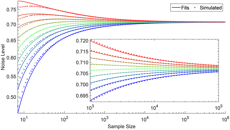
Figure 6. Relationship between distribution noise d_DN and sample size N at deciles going from the 10th percentile (blue) to the 90th (red), obtained from 10⁶ simulations. The d_DN value converges to $1/\sqrt{2}$ as N increases.

4.2. Relationship between Distribution Noise and KS Distance

As measures for statistical deviations, d_DN and d_KS are different in that d_DN measures deviation at the probability density level, whereas the d_KS measure it at the cumulative density level. As a result, d_KS assigns more weight to the tail of the distribution, while d_DN is more sensitive to deviations in the body of the distribution. Therefore, if we wish to combine these two measures to estimate the significance level, we need to first investigate the relationship between d_KS and d_DN. We do this by simulating 10⁶ samples from U(0, 1) for various sample sizes, and for each sample, we calculate d_KS and d_DN using Equations (4) and (18) respectively, to obtain 10⁶ pairs of d_KS and d_DN. We then compute the Pearson correlation between d_KS and d_DN and learned that (see Supplementary Information section 2 for the comparison of fits)

$\begin{array}{cc}{\rho }_{d_{KS},d_{DN}}(N)=\frac{e}{N^{0.481}}.& (21)\end{array}$

As expected, d_KS is positively correlated with d_DN. Since d_KS is a measure at the cumulative level, the random distribution noises cancel each other, thus the correlation between d_KS and d_DN vanishes as N → ∞.

5. Application to Significance Testing

5.1. Significance Level for a Given Distribution

To perform significance testing given d_KS and d_DN, we need the percentile values ℘_KS and ℘_DN. ℘_KS can be obtained by inverting Equation (16), as

$\begin{array}{cc}{\wp }_{KS}(d_{KS},N)=\frac{100}{\left(1+{\left(d_{KS}{N}^{0.492}\exp (0.274)\right)}^{-\frac{1}{0.176}}\right)}.& (22)\end{array}$

Similarly, we invert Equation (19), and solve

$\begin{array}{c}{\wp }_{DN}^{0.430}+{\left(50-{\wp }_{DN}\right)}^{0.302}\ln (|\eta |N^{0.495})=0,\eta <0\\ {\wp }_{DN}-50=0,\eta =0\\ {\left(100-{\wp }_{DN}\right)}^{0.430}+{\left({\wp }_{DN}-50\right)}^{0.302}\ln (|\eta |N^{0.495})=0,\eta >0& (23)\end{array}$

to get ℘_DN, where η = d_DN − 〈d_DN〉.

Substituting the empirical KS distance $d_{KS}^{(em)}$ and empirical distribution noise $d_{DN}^{(em)}$ into Equations (22) and (23), we obtain ${\wp }_{KS}^{(em)}$ and ${\wp }_{DN}^{(em)}$. This is an alternative way of obtaining the p-value without the need to perform Monte-Carlo (re)sampling again (CSN method), since we have already done so in sections 3 and 4. The percentage of simulated U(0, 1) samples with $d_{KS/DN}>d_{KS/DN}^{(em)}$ is $100-{\wp }_{KS/DN}^{(em)}$. Since d_KS and d_DN are not independent (Equation 21), we discount the correlation between d_KS and d_DN, and define the significance level (p-value) as

$\begin{array}{cc}p({\wp }_{KS},{\wp }_{DN},N)=\sqrt{\left(1-\frac{{\wp }_{KS}}{100}\right)\left(1-\frac{{\wp }_{DN}}{100}\right)\left(1-\frac{e}{N^{0.481}}\right)},& (24)\end{array}$

to avoid overestimating the significance level.

5.2. Fitting to Empirical Data

We follow the steps outlined in the CSN algorithm (section 2) to fit the empirical data, but with two important modifications: (Ii) the parameters (CSN(ib)) and goodness of fit (CSN(iib)) are adjusted for the finite largest element; and (Iii) the p-value (CSN(ivc)) is adjusted for the finite number of elements effect. Meanwhile, optional modifications are (Oi) to incorporate distribution noise as another dimension for goodness of fit, so that the p-value can be determined via $d_{KS}^{(em)}$, $d_{DN}^{(em)}$, or both; (Oii) instead of using bootstrapping to determine the p-value in the CSN method, which is very slow for large samples, one can use the fast inversion formulae Equations (22), (23), or (24).

Figure 7 shows the fits and p-testing results for Taiwan housing price, Taiwan wealth, and Straits Times Index normalized returns. It is reassuring that after modifications the p-values of all distributions increased. In particular, the two distributions (Figures 7B,C) that did not meet the p > 0.1 criterion (as suggested by Clauset et al. [24]) before modification, now have p > 0.5. This is in agreement with our visual assessment of the three fits. We also understand now that a large δ (small x_max) is the main reason for Taiwan wealth to fail p-testing before adjustment (although the fit is visually good). In general, our correction formulas perform the best when δ is large due to small sample sizes or truncations. Readers can refer to Supplementary Information section 4 for more plots and instances where small δ values affects the significance testing.

FIGURE 7

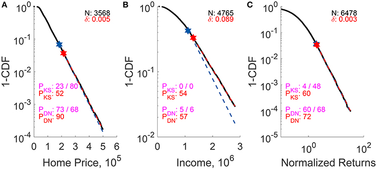
Figure 7. p-testing results for (A) 2012–2014 Taiwan home price per square foot (fitted to EXP), (B) 2012 Taiwan lower-tail income (fitted to EXP), and (C) 2009–2016 Straits Times Index normalized return (fitted to PL) before and after finite-sample adjustments. In this figure, the N represent the number of fitted data, and the empirical CDF that is adjusted for FLE is shown as black dots, while the unadjusted and adjusted fits are shown as blue and red dashed line respectively. P_KS/DN-values (in percentage) are for unadjusted (blue) and adjusted (red) fits. We separate the p-values obtained using the CSN method (left) from those using Equations (21) or (23) (right) by a “/”.

There are several limitations one should note while obtaining P_KS/DN using Equations (22) or (23). First, it is only applicable to large samples (see Figures 4, 6). Second, these equations are obtained after experimenting with several functional forms and are only approximate. Lastly, p_KS measured using the CSN method are consistently smaller than that based on Equation (22). This is due to the CSN algorithm having an extra step to select x_min that minimizes d_KS of each simulated sample, and thus the algorithm is stricter than our fast inversion formulae. However, the inversion formulae Equations (22) and (23) are convenient and provide an upper bound for P_KS/DN. We make the codes for the procedures used in parameter estimation and significance testing available at https://github.com/BoonKinTeh/StatisticalSignificanceTesting for both these two methods, but leave it to the reader to decide which method to use.

All in all, when we test for statistical significance, we need to be aware of finite sample effects, namely the finite largest element effect and the finite number of elements effect. Beyond the KS distance measured at the cumulative distribution level, we also introduce an alternative measure of the goodness of fit based on the distribution noise at the probability density level.

Author Contributions

BT, DT, and SC: designed research. BT: performed research. BT, DT, and SL: collected data. BT and DT: analyzed data. All authors wrote and reviewed the paper.

Funding

This research is supported by the Singapore Ministry of Education Academic Research Fund Tier 2 under Grant Number MOE2015-T2-2-012.

Conflict of Interest Statement

The authors declare that the research was conducted in the absence of any commercial or financial relationships that could be construed as a potential conflict of interest.

Acknowledgments

The authors would like to thank Chou Chung-I for directing us to the Taiwanese data sets.

Supplementary Material

The Supplementary Material for this article can be found online at: https://www.frontiersin.org/articles/10.3389/fams.2018.00002/full#supplementary-material

References

1. Kac M, Kiefer J, Wolfowitz J. On tests of normality and other tests of goodness of fit based on distance methods. Ann Math Stat. (1955) 26:189–211. doi: 10.1214/aoms/1177728538

CrossRef Full Text | Google Scholar

2. D'Agostino RB. Transformation to normality of the null distribution of g1. Biometrika (1970) 57:679–81.

Google Scholar

3. Jarque CM, Bera AK. A test for normality of observations and regression residuals. Int Stat Rev. (1987) 55:163–72.

Google Scholar

4. Shaphiro S, Wilk M. An analysis of variance test for normality. Biometrika (1965) 52:591–611.

5. Anderson TW, Darling DA. Asymptotic theory of certain “goodness of fit” criteria based on stochastic processes. Ann Math Stat. (1952) 23:193–212. doi: 10.1214/aoms/1177729437

CrossRef Full Text | Google Scholar

6. Anderson TW, Darling DA. A test of goodness of fit. J Am Stat Assoc. (1954) 49:765–9.

Google Scholar

7. Massey, FJ Jr. The Kolmogorov-Smirnov test for goodness of fit. J Am Stat Assoc. (1951) 46:68–78.

Google Scholar

8. Lilliefors HW. On the Kolmogorov-Smirnov test for normality with mean and variance unknown. J Am Stat Assoc. (1967) 62:399–402.

Google Scholar

9. Razali NM, Wah YB. Power comparisons of Shapiro-Wilk, Kolmogorov-Smirnov, Lilliefors and Anderson-Darling tests. J Stat Model Anal. (2011) 2:21–33.

Google Scholar

10. Newman ME. Power laws, Pareto distributions and Zipf's law. Contemp Phys. (2005) 46:323–51. doi: 10.1016/j.cities.2012.03.001

CrossRef Full Text | Google Scholar

11. Mantegna RN, Stanley HE. Scaling behaviour in the dynamics of an economic index. Nature (1995) 376:46–9.

Google Scholar

12. Plerou V, Gopikrishnan P, Amaral LAN, Meyer M, Stanley HE. Scaling of the distribution of price fluctuations of individual companies. Phys Rev E (1999) 60:6519.

PubMed Abstract | Google Scholar

13. Gopikrishnan P, Plerou V, Amaral LAN, Meyer M, Stanley HE. Scaling of the distribution of fluctuations of financial market indices. Phys Rev E (1999) 60:5305.

PubMed Abstract | Google Scholar

14. Teh BK, Cheong SA. The Asian correction can be quantitatively forecasted using a statistical model of fusion-fission processes. PloS ONE (2016) 11:e0163842. doi: 10.1371/journal.pone.0163842

PubMed Abstract | CrossRef Full Text | Google Scholar

15. Zipf GK. Human Behavior and the Principle of Least Effort. Reading, MA: Addison-Weslay (1949).

Google Scholar

16. Cancho RFi, Solé RV. The small world of human language. Proc R Soc Lond B Biol Sci. (2001) 268:2261–5. doi: 10.1098/rspb.2001.1800

CrossRef Full Text | Google Scholar

17. Auerbach F. Das gesetz der bevölkerungskonzentration. Petermanns Geogr Mitt. (1913) 59:74–6.

Google Scholar

18. Gabaix X, Ioannides YM. The evolution of city size distributions. Handb Region Urban Econ. (2004) 4:2341–78. doi: 10.1016/S1574-0080(04)80010-5

CrossRef Full Text | Google Scholar

19. MacKay N. London house prices are power-law distributed. arXiv preprint arXiv:10123039 (2010).

Google Scholar

20. Ohnishi T, Mizuno T, Shimizu C, Watanabe T. Power laws in real estate prices during bubble periods. Int J Mod Phys Conf Ser. (2012) 16:61–81. doi: 10.1142/S2010194512007787

CrossRef Full Text | Google Scholar

21. Tay DJ, Chou CI, Li SP, Tee SY, Cheong SA. Bubbles are departures from equilibrium housing markets: evidence from Singapore and Taiwan. PLoS ONE (2016) 11:e0166004. doi: 10.1371/journal.pone.0166004

PubMed Abstract | CrossRef Full Text | Google Scholar

22. Mandelbrot B. The Pareto-Levy law and the distribution of income. Int Econ Rev. (1960) 1:79–106.

Google Scholar

23. Yakovenko VM, Rosser JB Jr. Colloquium: statistical mechanics of money, wealth, and income. Rev Mod Phys. (2009) 81:1703. doi: 10.1103/RevModPhys.81.1703

CrossRef Full Text | Google Scholar

24. Clauset A, Shalizi CR, Newman ME. Power-law distributions in empirical data. SIAM Rev. (2009) 51:661–703. doi: 10.1137/070710111

CrossRef Full Text | Google Scholar

25. Brzezinski M. Do wealth distributions follow power laws? Evidence from “rich lists”. Phys A (2014) 406:155–62. doi: 10.1016/j.physa.2014.03.052

CrossRef Full Text | Google Scholar

26. Hansen LP, Heaton J, Yaron A. Finite-sample properties of some alternative GMM estimators. J Bus Econ Stat. (1996) 14:262–80.

Google Scholar

27. Windmeijer F. A finite sample correction for the variance of linear efficient two-step GMM estimators. J Econom. (2005) 126:25–51. doi: 10.1016/j.jeconom.2004.02.005

CrossRef Full Text | Google Scholar

28. Fisher RA. On an absolute criterion for fitting frequency curves. Messenger Math. (1912) 41:155–60.

Google Scholar

29. Kumphon B. Maximum entropy and maximum likelihood estimation for the three-parameter Kappa distribution. Open J Stat. (2012) 2:415–9. doi: 10.4236/ojs.2012.24050

CrossRef Full Text | Google Scholar

30. Hradil Z, Rehácek J. Likelihood and entropy for statistical inversion. J Phys Conf Ser. (2006) 36:55. doi: 10.1088/1742-6596/36/1/011

CrossRef Full Text | Google Scholar

31. Akaike H. Information theory and an extension of the maximum likelihood principle. Chapter 4: AIC and Parametrization. In: Parzen E, Tanabe K, Kitagawa G, editors. Information Theory and an Extension of the Maximum Likelihood Principle. New York, NY: Springer New York (1998). p. 199–213.

Google Scholar

32. Bates DM, Watts DG. Nonlinear Regression Analysis and Its Applications. New York, NY: Wiley (1988).

33. Wooldridge JM. Applications of generalized method of moments estimation. J Econ Perspect. (2001) 15:87–100. doi: 10.1257/jep.15.4.87

CrossRef Full Text | Google Scholar

34. Cameron AC, Windmeijer FAG. An R-squared measure of goodness of fit for some common nonlinear regression models. J Econom. (1997) 77:329–42.

Google Scholar

35. Janczura J, Weron R. Black swans or dragon-kings? A simple test for deviations from the power law. Eur Phys J Spec Top. (2012) 205:79–93. doi: 10.1140/epjst/e2012-01563-9

CrossRef Full Text | Google Scholar

36. American Statistical Association. ASA P-Value Statement Viewed > 150, 000 Times. American Statistical Association News (2016). (Accessed March 07, 2017). Available online at: https://www.amstat.org/ASA/News/ASA-P-Value-Statement-Viewed-150000-Times.aspx

37. Wasserstein RL, Lazar NA. The ASA's statement on p-values: context, process, and purpose. Am Stat. (2016) 70:129–33. doi: 10.1080/00031305.2016.1154108

CrossRef Full Text | Google Scholar

38. Baker M. Statisticians issue warning over misuse of P values. Nature (2016) 531:151. doi: 10.1038/nature.2016.19503

PubMed Abstract | CrossRef Full Text

39. Pitman EJ, Pitman EJG. Some Basic Theory for Statistical Inference, Vol. 7. London: Chapman and Hall London (1979).

40. Alstott J, Bullmore E, Plenz D. powerlaw: a Python package for analysis of heavy-tailed distributions. PLoS ONE (2014) 9:e85777. doi: 10.1371/journal.pone.0085777

PubMed Abstract | CrossRef Full Text | Google Scholar

41. Yu S, Klaus A, Yang H, Plenz D. Scale-invariant neuronal avalanche dynamics and the cut-off in size distributions. PLoS ONE (2014) 9:e99761. doi: 10.1371/journal.pone.0099761

PubMed Abstract | CrossRef Full Text | Google Scholar

42. Marshall N, Timme NM, Bennett N, Ripp M, Lautzenhiser E, Beggs JM. Analysis of power laws, shape collapses, and neural complexity: new techniques and Matlab support via the ncc toolbox. Front Physiol. (2016) 7:250. doi: 10.3389/fphys.2016.00250

PubMed Abstract | CrossRef Full Text | Google Scholar