The Amnesiac Lookback Option: Selectively Monitored Lookback Options and Cryptocurrencies

1. Introduction

Lookback options have been a prototypical example of exotic options within the financial literature [1]. The option gives the holder the right to buy or sell an underlying asset at any price attained within a specified “lookback” period. The payoff of a lookback call (put) is therefore the difference between the underlying price at maturity and the maximum (minimum) price attained. The trader is thus able to capitalize on the underlying asset as if he sold it at the optimal time. By utilizing only the highest value of the underlying asset in determining payoff, lookback options capture the best case scenarios that people would like to sell at, but often miss due to uncertainty. By corresponding payoffs to the extreme movements of underlying asset prices, lookback options allow for investors to hedge against or invest in volatility.

Goldman et al. [2] [3] are one of the first who mentioned the lookback option within the financial literature. Their paper examines the properties of path-dependent European options under Black-Scholes assumptions. They laid out three primary motivations: to minimize regret, to live out the “fantasy” of buying low and selling high, and lastly, to use knowledge of the range to expand an investors opportunity set. This last condition is only applicable within the realistic market setting rather than a frictionless one. The nature of lookback options also lets investors guard against the behavioral flaws in people. The nature of lookback options also lets investors guard against the behavioral flaws in people. Because the payoffs of lookbacks are path dependent in a way to capture the effects of the best prices, lookbacks can hedge not only quantitative variations in the market, but irrational regret of the human mind.

Lookback options benefit the holder given greater volatility in the market. Thus, it is an effective instrument for hedging against large price movements and reducing the risk of destabilizing events that may cause markets to either rise or fall. These include political election outcomes or other unforeseen chance occurrences such as market anomalies [4]. Also among its potential uses is to hedge exposure in cryptocurrency markets, where extreme volatility has increasingly become a menace as investors look for ways to mitigate such risk.

However, the lookback option's strong reduction to risk exposure requires a sufficiently high premium, which reduces the option's demand. The proposition of this paper recognizes that one may not have to look back upon the entire associated time period; merely looking back upon a portion suffices to capture most of the max potential payoff of a full-time lookback option, most of the time. This conclusion allows for investors to adjust their risk using lookbacks of differing lookback period lengths by purchasing shorter time lookback options at a discount in order to increase return on investment. This strategy suggests the possibility of event-based trading whereby lookback periods may be chosen to correspond to market shaping events in hopes of extraordinary profits.

As the potential payoffs and insurance capabilities of an option increase, so does its premium. Thus, there is a desire for an instrument that limits risk exposure, but at a lower price. Here is where the proposed “Amnesiac Lookback Option” may find a tradeable niche, a variant of the conventional lookback option whose lookback time periods are restricted to a chosen subset of periods within a specified time interval at the time the contract is created. If premiums for lookbacks may be reduced, it could also open the door for their widespread use, particularly in high volatility cryptocurrency markets. The purpose of this study is therefore 2-fold: to propose a way to make the lookback option cheaper and more practical, and suggest the use of its properties to reduce risk exposure in cryptocurrency markets and correct for informational inefficiencies surrounding prices and volatility. Additionally, we are interested in the following research questions. What periods of the amnesiac lookback option should be selected to maximize its final payoff? What is the probability that the amnesiac lookback option may produce greater profit than the standard lookback option? Lastly, would this option have practical applications in the cryptocurrency market?

The rest of the paper is organized in the following way: The rest of the introduction provides more context on the varieties of lookback options and applications to cryptocurrencies. Section 1 continues to discuss types of lookbacks and its application to the cryptocurrency market. Section 2 discusses existing literature on partial lookback options, lookback options with diluted premiums, and past efforts to price them. It then discusses our methods of simulation. Section 3 presents the results of three types of numerical simulations. First, a demonstration of the general properties of floating amnesiac lookback options for calls, puts and spread options are shown. Second, the payoff of fixed strike amnesiac lookback options is shown and compared to the fixed strike. Third, a study of equidistant monitoring vs. two forms of random monitoring are presented. Section 4 prices different cryptocurrency using the algorithm in conjunction with smart contracts.

1.1. Fixed vs. Floating Lookback Options

Lookbacks exist in many different varieties but can be classified into two broad categories: fixed and floating strikes. The strike price of fixed strikes is indicated in the initial contract, while for floating strike lookbacks the strike price is the minimum (call) or maximum (put) of the underlying asset. Additionally, there are spread lookback options with payoffs equal to the difference between the maximum and minimum prices attained by the underlying. The payoffs are summarized in Table 1 where $M_0^T=max{\left\{S_i\right\}}_{i=0}^T$ and $m_0^T=min{\left\{S_i\right\}}_{i=0}^T$. T denotes the time of maturity.

TABLE 1

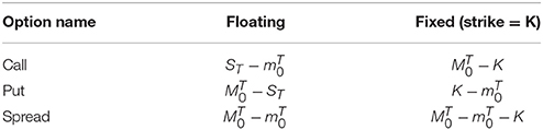
Table 1. Payoffs for floating and fixed strike lookback options.

Suppose an investor decides to take the long position for the next 2 months. However, the price of the stock drops unexpectedly within the last 4 days of closing by 10%. Not selling the stock early becomes a reason of regret. Similarly, the stock may drop in the span of 2 days before rising quickly, making the investor regret not buying the stock a little later. Thus the floating strike call lookback is useful for market exit and the fixed strike call for market entry.

1.2. The Partial and the Amnesiac

Due to the high premiums of lookback options and perhaps other factors, lookback options are not sold at particularly high volumes within OTC trades [5]. It has been suggested that partial lookback options may allow lookbacks to be more tradeable. One such way is to introduce a factor λ that decreases the effect or payoff of the lookback, proposed by Conze and Viswanathan [6]. For instance, the payoff of such an instrument is:

$\begin{array}{cc}\lambda (\max {\left\{S_i\right\}}_1^N-S_T)& (1)\end{array}$

If λ equals 1 then payoff is identical to a standard lookback option. Another form of the partial lookback, referred to as the fractional lookback, restricts the lookback periods to a continuous subset of days. Finally there is also the window lookback option, where separated continuous periods are monitored [7].

The amnesiac lookback option generalizes partial and discrete lookback options that are not linearly reliant on the payoff of the standard lookback option and is named such in response to Heynen and Kat's paper Selective Memory. The amnesiac lookback option is a lookback option whose lookback periods belong to a pre-specified subset of periods from a given time interval, determined at the moment of contract creation.

The amnesiac lookback option is thus defined as follows. Given a full, discrete lookback option with N total lookback periods, an amnesiac option is defined by a subset of periods of the full, discrete lookback option, denoted as A. The payoff scheme is the same as the standard lookback, while the extreme values of the option are restricted to A. This means, every full, discrete lookback option is in fact an amnesiac option of a full lookback with greater periods. This extends previous definitions of partial lookbacks to beyond equidistant intervals.

1.3. Application to Cryptocurrencies

Lookback options are extremely suited to hedge against volatility in general, whether the underlying asset surges in value, or whether the underlying asset declines in value. Unpredictability is therefore the prime feature of an asset that would drive demand and usage for a lookback option based upon that asset. In 1982, the Mocatta Metals Corporation issued one of the first “lookbacks,” that allowed a trader to buy gold at the lowest price attained within a period. In the context of modern day financial markets, it would seem lookbacks could have high potential in hedging investments involving the popular digital gold cryptocurrencies. A pioneering innovation within currency markets, instruments such as Bitcoin and Ethereum may represent the future of monetary exchange. Given its relative technology security, explosion in value, and increasing acceptance of legitimacy, Carrick [8] has even suggested that cryptocurrencies like Bitcoin could be used as a complement to fiat currencies in emerging markets. At the same time, high volatility has become the premier feature of cryptocurrency markets, which has made investment risky. A Bitcoin was worth $2 in 2011—and exploded to $4,000 in 2017 [9]. During that time, volatility for daily returns would regularly exceed 10%, even skyrocketing to 16% [10]. Bitcoin once lost 75% of its value over 2 years, and then rising 2,000% within the next two.

Past literature has found evidence of time series characteristics and long memory behavior in Bitcoin markets, both in regards to pricing and in return volatility. Bariviera et al. [11] explores some of these inefficiencies by calculating Hurst exponents via the Detrended Fluctuation Analysis method for certain time windows of Bitcoin return and return volatility data. Bariviera finds evidence that from 2011 to 2014, daily Bitcoin returns had long-term positive autocorrelation with previous returns and that return volatility had long memory throughout the entire time period of 2011–2017 [11]. Bariviera et al. [11] utilize this same methodology to further show that intraday returns before 2014 exhibit long range memory as well. Additionally, Urquhart [12] finds that Bitcoin prices exhibit odd behaviors through the entire time period May 2012 to April 2017, with over 10 percent of prices ending with decimal digits of 00. One, two, three, five, and ten days before a round number from rising prices, returns are positive and statistically significant. Meanwhile, prices after a round number show no such predictable behaviors. Given that the lookback option utilizes the time series behavior of an asset's prices and volatility to determine its payoff, it is a suitable candidate for rectifying such market inefficiencies. The amnesiac lookback option is particularly appropriate because lookback period selection allows for targeted correction of unusual events, such as those found in Urquhart [12], and can more easily eliminate arbitrage opportunities and bring markets into more efficient states.

Ultimately, Bitcoin aims to be a type of fiat money; it has no value backed with consumable goods and its value comes from the minds of its investors and from the financial environment in which it occupies. Increases have been driven by hopes of future value, or in other terms, heavy speculation. Unexpected events therefore have rippling effects on the cryptocurrency market and create a volatility with few equal comparisons. China's decision to cease its bitcoin exchange in September of 2017 sent Bitcoin into a downward spiral, and as governments and regulators venture forth into the frontier that is the cryptocurrency market, events that will shock the market are sure to take place [13]. Even so, investors are increasingly accepting of cryptocurrencies as attractive investment propositions outside of speculation. Bouri et al. [14] find that Bitcoin can act as a hedge against market uncertainty in situations, specifically in short time horizons under extreme bear or bull market regimes, or when uncertainty is either very low or very high. Bouri et al. [15] overall minimizes the usefulness of Bitcoin as a general hedge, but still finds evidence that investors put money into Bitcoin when Asian stocks experience extreme down movements.

In July 2017, the U.S. Commodity Futures Trading Commission granted federal approval to LedgerX LLC for the ability to trade and exchange options based on cryptocurrency [16]. This happening marked the birth of the first federally regulated platforms of cryptocurrency options trading, and moved items such as Bitcoin, Ethereum, and even Dogecoin closer into the realm of financial legitimacy. Shortly after on December 1, 2017, the U.S. Commodity Futures Trading Commission announced the offering of self-certified derivatives from three financial firms: bitcoin futures from the Chicago Mercantile Exchange Inc. and the CBOE Futures Exchange and binary options from the Cantor Exchange [17]. In contrast with the effect of regulatory restrictions, this decision has driven up bitcoin prices from $5,000 prior to the announcement to above $11,000 by December 05, 2017 [18]. The issuance of new financial instruments can thus feedback into the price of its underlying.

More importantly, the integration of smart contracts into blockchain technology has vastly expanded the possibilities of options trading, allowing traders great flexibility in designing their own options [19–21]. Smart contracts are computer protocol that allow for trade and exchange without the need for an intermediary, and because writers code their own contracts, blockchain technology can facilitate the trade of highly customized contracts often seen on the OTC market. Both Bitcoin and Ethereum, for instance, support programming languages that allow for the creation of custom smart contracts [22, 23]. Amnesiac lookback options could conceivably exist within this structure, and be traded as a smart contract.

Recent events lent credence to the prospect of a prolific smart contract exchange. In March 2018. The state of Tennessee signed into law a bill that recognizes smart contracts as having legal power [24], providing a pathway for other states to follow and further securing the legitimacy of these digital arrangements. Blockchain based smart contract firm Hedgy has also created irrefutable and unalterable “Smart Futures” that can enforce digital obligations and streamline settlements [25]. As more and more investors begin creating and trading new smart contracts, blockchain may 1 day even “democratize” the OTC market and open a plethora of new smart instruments to be exchanged.

Lookback options therefore emerge as an attractive and easily implementable product for currency speculators. As price fluctuation is the determining factor of payoff, such lookback instruments would be highly priced in the cryptocurrency market and be a key counterweight to the speculative risk of investors. Simple to understand and able to exist as smart contracts, lookback options and other path-dependent options could serve as a unique tool for traders with restricted access to dynamic trading strategies, and in the process introduce greater flows of capital from these sources to promising investments.

2. Materials and Methods

2.1. Past Pricing Model for Lookbacks

Research with lookback options fall within pricing methods for path dependent exotic options, such as the barrier option which also rely on extreme value processes, and the Asian option which relies on the average price of the underlying. Goldman introduced the instrument into the financial literature in 1979 [2, 3]. Following Black, Scholes and Merton's pricing of vanilla options, Black-Scholes assumptions have been extended to price exotic options. This is defined by at least one asset with price S that moves under Geometric Brownian Motion with constant drift and volatility. The underlying price follows:

$\begin{array}{cc}dS=S\mu dt+\sigma SdX& (2)\end{array}$

where the underlying has drift μ and volatility σ. In the risk-neutral measure, the stock price at a given time t and final time T is given below:

$\begin{array}{cc}{S}_{t+1}=S_t{e}^{(r-D-\frac{{\sigma }^2}{2})\Delta t+\sigma ϵ\sqrt{\Delta t}}& (3)\end{array}$

$\begin{array}{cc}{S}_T=S_0{e}^{(r-D-\frac{{\sigma }^2}{2})T+\sigma ϵ\sqrt{T}}& (4)\end{array}$

r denotes the risk free rate, σ the volatility, D denotes dividends in the case of stocks, and $ϵ~{N}(0,1)$, the normal distribution.

Like the Vanilla European Option, an analytic pricing formula has been shown using martingale methods [26], with the price of a call given as:

$\begin{array}{cc}\begin{array}{l}{C}_t=S\Phi (a_1(S,m))-m{e}^{-r\tau }\Phi (a_2(S,m))-\frac{S{\sigma }^2}{2r}(\Phi (-a_1(S,m))\\ -e^{-r\tau }{\left(\frac{m}{S}\right)}^{\frac{2r}{{\sigma }^2}}\Phi (-a_3(S,m)))\end{array}& (5)\end{array}$

$\begin{array}{cc}\begin{array}{l}{P}_t=-S\Phi (-a_1(S,M))+M{e}^{-r\tau }\Phi (a_2(S,M))+\frac{S{\sigma }^2}{2r}(\Phi (a_1(S,M))\\ -e^{-r\tau }{\left(\frac{M}{S}\right)}^{\frac{2r}{{\sigma }^2}}\Phi (a_3(S,m)))\end{array}& (6)\end{array}$

where M denotes the running maximum at time t, m denotes the running minimum,τ = T−t with T the time of maturity, and Φ the standard normal cumulative distribution function given as

$\Phi (\alpha )=\frac{1}{\sqrt{2\pi }}{\displaystyle {\int }_{-\infty }^{\alpha }{e}^{-\frac{x^2}{2}}}dx$

With L being a dummy variable, the variables denote:

$\begin{array}{l}{a}_1(S,L)=\frac{\ln \frac{S}{L}+(r+\frac{1}{2}{\sigma }^2)\tau }{\sigma \sqrt{\tau }}\\ a_2(S,L)=a_1(S,L)-\sigma \sqrt{\tau }\\ a_3(S,L)=a_1(S,L)-\frac{2r\sqrt{\tau }}{\sigma }\text{for }L>0,S>0\end{array}$

For fixed strikes, Conze and Vishwanathan [6] used known properties of maxima and minima distributions to price the lookback call, under the continuous case of lookback periods.

$C_t=\{\begin{array}{ll}{S}_0\Phi (b(T))\hfill & -e^{rT}K(b(T)-\sigma \sqrt{T}+e^{-rT}\frac{{\sigma }^2}{2r}{S}_0(e^{rT}\Phi (b(T))\hfill \\ \hfill & -{(\frac{S_0}{K})}^{\frac{-2r}{{\sigma }^2}}\Phi (b(T)-\frac{2r}{\sigma }\sqrt{T}))K\ge M\hfill \\ e^{rT}(M_T^0-\hfill & K)+S_0\Phi (b^{\prime }(T))-e^{-rT}{M}_T^0\Phi (b^{\prime }(T)-\sigma \sqrt{T})\hfill \\ \hfill & +e^{-rT}\frac{{\sigma }^2}{2r}{S}_0(e^{rT}\Phi ({d^{\prime }}_T)-{(\frac{S_0}{M_T^0})}^{\frac{-2r}{{\sigma }^2}}\Phi (b^{\prime }(T))\hfill \\ \hfill & -(\frac{2r}{\sigma }\sqrt{T})K<M\hfill \end{array}$

where

$\begin{array}{cc}\begin{array}{l}b(T)=\frac{\ln \frac{S_0}{K}+(r-D+\frac{{\sigma }^2}{2})T}{\sigma \sqrt{T}}\\ b^{\prime }(T)=\frac{\ln \frac{S_0}{M_0^T}+(r-D+\frac{{\sigma }^2}{2})T}{\sigma \sqrt{T}}\end{array}& (7)\end{array}$

The similar case for the put is derived in their paper, and resembles the form of the float-strike option in Equation (5). These analytic solutions assume continuous monitoring and updates to the price of the underlying, while in reality most options are monitored at discrete intervals. Thus, the analytic solutions are typically overpriced as compared to the prices of discretely monitored lookbacks, and has spurred two areas of study: how to either price discrete options more accurately, and how to correct errors of continuous monitoring.

Historically, notable papers that have priced discrete lookback options include those by Heynen and Kat using the Black-Scholes model [27], Babbs using a binomial valuation [28], and Cheuk and Vorst [29] using a binomial model. More recent pricing paradigms utilize stochastic volatility [30] and the Lévy Model [31] (more citations here). Cheuk and Vorst in particular consider the effects of observation frequency on price using equal lookback intervals.

The binomial options pricing model first described in Cox et al. [32] offers a conceptual method with which the price of an amnesiac lookback options may be determined. Under the assumptions of the binomial tree model, the price of an underlying stock S_t at discrete time t may strictly exhibit one of two behaviors. It may either increase in value to S_tu with probability p, or decrease in value to S_td with probability q where $u=e^{\sigma \sqrt{t}}$, d = 1/u, p+q = 1, and sigma is a measure of the stock's volatility. The risk-neutral probability p is determined to equal $\frac{e^{(r\Delta t)}-d}{u-d}$ where r an exogenously determined risk free return. The lookback option can then be priced recursively using a lattice.

This pricing model was then extended to be more efficient by Conze and Vishwanathan [6], Babbs [28], and Cheuk and Vorst [29]. The binomial pricing method lends itself more easily to pricing at discrete intervals. With too few time intervals, the approximation for the standard lookback option becomes inaccurate. Yet as the number of periods in the binomial tree increases, so does the amount of computations. Past work involves increasing the efficiency of these computations using combinatorial properties of the binomial tree. Babbs [28] uses a change of numeraire approach, similar to Hull and White [33], to price both new and existing lookback options. Cheuk and Vorst formulate a modified tree, where the computation only relies on time and the difference between u and d. Let this variable be called j such that:

$\begin{array}{cc}{S}_t=(\underset{t\le T}{\min }{S}_t)u_n^j{S}_t=(\underset{t\le T}{\max }{S}_t)u_n^{-j}& (8)\end{array}$

for the call and the put respectively. Then the price for a floating strike lookback can be given as $C_n^{fl}=S_0{V}_n(0,0)$, where:

$\begin{array}{cc}{V}_n(0,0)={\displaystyle \sum _{j=0}^n(1-u_n^{-j})}P(V_{0,n}^{*}=0,V_n^{*},n=j)& (9)\end{array}$

The notation star such as in $V_{m,n}^{*}$ denotes for n fixed and 0 < m < n. The probabilities are given by:

$\begin{array}{cc}\begin{array}{l}P(V_{0,n}^{\ast }=0,V_n^{*},n=j)={\displaystyle \sum _{k=j}^l\Lambda }j,k,m{\left(1-q_n\right)}^k{q}_n^{m-k}\\ \text{ for}\Lambda j,k,m=\left(\begin{array}{c}m\\ k-j\end{array}\right)-\left(\begin{array}{c}m\\ k-j-1\end{array}\right)\end{array}& (10)\end{array}$

if k > j and Λj, k, m = 1 is k = j.

While both the modified tree model and the analytic formula give continuous valuation results, and it is well known the binomial tree model converges to the continuous price. the pricing formulae is still related to discrete lookback pricing. Cheuk and Vorst extended the total number of lookback periods, then selected an equal-distant subset to model the discrete monitoring periods. Similarly, the amnesiac lookback option is defined on a subset of monitoring periods.

Upon noting the discrepancy between continuous and discrete monitoring pricing assumptions, researchers continued to improve methods of pricing discrete options. Aitsahlia and Le Lai [34] uses the random walk duality to simplify recursive integration. Petrella and Kou [35] uses the Laplace transform to make pricing more efficient, and Broadie et al. [36] uses approximation adjustments to the continuous case to fairly price the option's discrete counterpart.

Contemporary researchers derive pricing under the framework of Lévy Processes, and as a natural extension, the Wiener-Hopf factorization is implemented as it gives the distribution of functionals within a random walk. Fusai et al. [37] combined this with Spitzer's identity for a general method of pricing discretely monitored exotic options, with an explicit formula for the fixed strike option. However, the method assumes equidistant monitoring windows. Boyarchenko and Levendorskii [38] similarly implement the Wiener-Hopf factorization but correct for the discrete monitoring dates using a Laplace transformation. Hieber [39] presents the general pricing of exotic options using the Fourier Transform and under Black-Scholes assumptions and regime switching model. This is not just useful for lookback options but for digital options and barrier options. However, the pricing scheme is for continuously monitored options. Feng and Linetsky [40] on the other hand, implements Hilbert transformations sequentially and presents an interesting method of computing maxima and minima, thereby applying it to the valuation of path-dependent options.

2.2. Method of Simulation

The definition of a amnesiac option in section 1 can be formalized as follows. Let N denote the total number of periods of a full lookback option. Let A denote a selected subset. Given a sequence of asset prices {S_i}, define $M_0^T$ the maximum and $m_0^T$ the minimum defined on the subsequence where i∈A. The payoff of the amnesiac option is then the same as Table 1.

To price the amnesiac lookback option, we utilize a Monte Carlo pricing simulation under the assumptions of the Black-Scholes world, including but not limited to, its modeling parameters, risk-free rate, dividends, and volatility. We assume geometric Brownian Motion under a risk-neutral measure as described in Equation (4):

$S_T=S_0{e}^{(r-D-\frac{{\sigma }^2}{2})T+\sigma ϵ\sqrt{T}}$

We assume dividends D = 0. We simulate this process using a Gaussian random walk. The algorithm is shown explicitly in Algorithm 1:

ALGORITHM 1

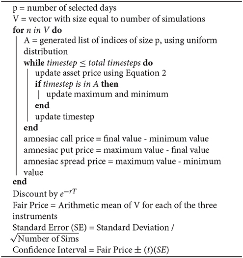
Algorithm 1: Algorithm for Pricing Amnesiac Option

where t is the corresponding t value for the confidence level. The updating of the asset price follows a Gaussian Random walk in Algorithm 2 where dT is the total time T divided by the number of selected days p:

ALGORITHM 2

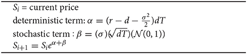
Algorithm 2: The price evolution based on the Gaussian Random Walk.

A denotes how the days are chosen. Our experiment features three forms of period selection: uniform random with fixed endpoints, completely random, and equal distant selection. For the amnesiac option with fixed endpoints, the first and last indices are first chosen, then indices 0 < i < N are chosen using the uniform distribution. For true random, indices are randomly selected under the uniform distribution with no guarantee of the first one being selected. For equal distant period selection, indices are chosen, and rounded down when not divisible. We make an assumption that on average, the population's selection of periods will be uniform random.

The parameters are shown in Table 2.

TABLE 2

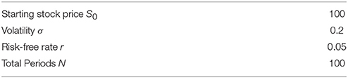
Table 2. Simulation parameters.

For each time step, the maximum and minimum value is updated. We analyze the pricing of floating and fixed amnesiac lookback options, along with the variants discussed in Table 1 (call, put, and spread). Then, the payoffs under equal interval sampling and random sampling are considered.

A useful function that appears in analysis is the general Hill Function. the Hill Function in the form:

$\begin{array}{cc}V(X)=\frac{V_{Max}{X}^h}{K^h+X^h}& (11)\end{array}$

The Hill Function has its roots in chemistry, where it is commonly used to model the kinetics of substrate reaction rate, where the x-axis is the substrate concentration and the y-axis the rate of reaction. V_Max is the maximal saturation rate, K denotes the value of x required to attain half of V_Max, x is the density of a substance, and h is the hill coefficient, as an exponential of K and h.

Analogously, increasing lookback periods yield diminishing returns to payoff and the components of the Hill Function give intuition to the process itself. Firstly, V_max is theoretically the maximum payoff, or the price of the standard discrete lookback option. Secondly, as we increase the starting stock price, both V_max and C scale linearly. On the other hand, both K and h remain constant and depend on interest rate r and volatility σ. The Hill Curve can thus price amnesiac lookbacks independent of the initial asset price, keeping interest and volatility constant. If the price of the standard lookback option V_max is known, and interest rate and volatility incorporated into K and h, then pricing can be done very efficiently using the Hill Equation. Additionally, the curve can be adopted to any starting stock price, since the initial stock price only influences V_max. The ratio between the price evolution and initial price is simply $\frac{S_0{e}^{(r-d-\frac{{\sigma }^2}{2})T+\sigma \sqrt{T}}}{S_0}=e^{(r-d-\frac{{\sigma }^2}{2})T+\sigma \sqrt{T}}$, hence when pricing under the same interest and volatility the payoff can simply be scaled.

The total number of simulations per parameter set is 2,000,000, the fair price being the arithmetic mean of the payoffs, with a target maximal standard error of 0.001.

3. Results

We denote C_n and P_n as the amnesiac option with n chosen monitoring periods. When unspecified, the monitoring regime is assumed to be random period monitoring with fixed endpoints.

3.1. Floating Strike Amnesiac Option

To reiterate the definition of an amnesiac lookback option, its payoff scheme is as described in Table 1, where only the maxima and minima of a subset of periods are recorded. We use T and t to denote the continuous case and N and n be the discrete case. Let N be the total number of periods and A the ordered set of indices:

$A=\{n_a,n_b,,n_N\}\forall A\subset N$

The amnesiac is defined on any k selected monitoring periods.

Figures 1, 2 show the payoff vs. the number of days selected. As the number of periods look backed on increases, the payoff approaches that of the standard lookback option. Yet it does not require many selected periods to capture most of the payoff of the full 100 selected days. This can be attributed to the diminishing marginal effect of additional selected periods; each period selected after the first contributes less additional payoff than the previous. For each data point, we took the mean of 2, 000, 000 simulations, and given a calculated Standard Deviation of around 14.54, this gives an error of around 0.01 in absolute terms.

FIGURE 1

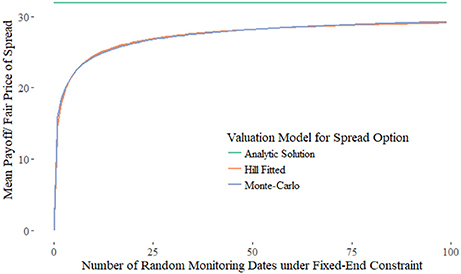
Figure 1. Monte-Carlo simulation for the Spread Option results converge to the Hill-Function with K = 1.18, h = 0.62, and V_max = 30.96.

FIGURE 2

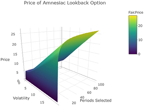
Figure 2. 3D Surface of the payoff varying days selected and volatility.

The sample errors are summarized in Table 3.

TABLE 3

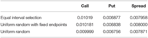
Table 3. Average of sample errors from 2,000,000 simulations.

Figure 1 fits the Hill function as previously described, and Figure 2 extends this to include volatility. For this particular case, the formula is observed to be:

$V(X)=\frac{30.96X^{0.62}}{{1.18}^{0.62}+X^{0.62}}$

Kernel density estimators further tell the differences of portfolios constructed from different amnesiac. Figure 3 shows the distribution of the call payoffs. The peak clustered at zero denotes the likely-hood of the option not being exercised, which yields a payoff of zero. Comparisons between instruments vary case-by-case, so it is useful in comparing expected returns in a pairwise fashion.

FIGURE 3

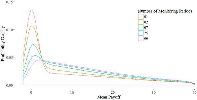
Figure 3. Distribution of payoffs for the call with bandwidth = 1.

Figure 4 shows the expected returns for the number of monitoring periods n equal to 99, 7, and 2. We define returns by the payoff minus the price of the option, which is the mean. Let x_i denote a single payoff from the simulation, then let the price of the call be defined as the average $\bar{X}$ then the returns are defined by:

$R=x_i-\overline{X}$

The payoff distribution of n = 7 for R > 0 is approximately the same as the distribution of n = 99. In fact, they converge in the negative region, hence their probability of R > 0 is approximately equal. Next, note that the downside of n = 99 is greater than that of n = 7. This means that the downside for C₇ is more limited than C₉₉, even if their conditional expectation for the downside is equal or even worse. This indicates that the amnesiac lookback, and partial lookbacks with less monitoring periods in general, can be used to limit the downside effects.

FIGURE 4

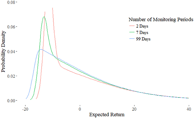
Figure 4. Distribution of the Expected Returns. Right tails converge, while for greater n left tails shifts out.

3.1.1. Three Types of Payoffs

Figure 5 shows the three payoff types as described in Table 1 for floating strikes, denoted in the first column. The sum of the fair-price of the call and put is equal to the spread option, which is why it is often described as a “double lookback option.”

FIGURE 5

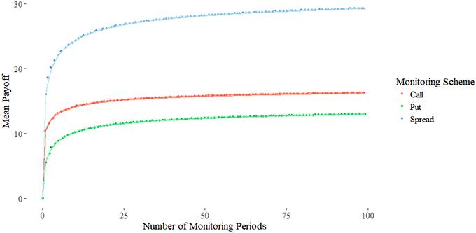
Figure 5. The payoffs of the put (blue), call (orange), and spread (gray). The payoff of the put and call sum to the spread. The put payoff is lower than the call as the absolute difference of the maximal processes is greater than the minimal processes under Geometric Brownian Motion.

FIGURE 6

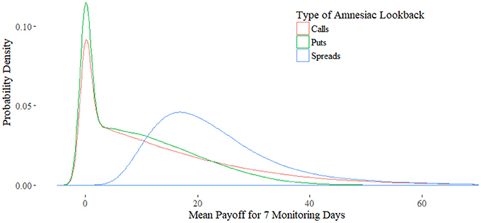
Figure 6. Kernel Density Estimation of each Amnesiac type. The tail behavior of the spread option is captured by the distribution of the call and puts.

Figure 5 also shows that the average maximal and minimal value is independent of the average final value. This observation can be illustrated as follows, given the payoffs in Table 1 and E the expectation operator.

$\begin{array}{cc}\begin{array}{l}E(call)+E(put)=E(S_{max}-S_T)+E(S_T-S_{min})\\ =E(S_{max}-S_T+S_T-S_{min})\\ =E(S_{max}-S_{min})=E(spread)\end{array}& (12)\end{array}$

These results show remarkable resemblance to the rate of convergence for exotic prices described in Dai et al. [41]. Indeed the prices produced by varying the number of total periods N follows a similar curve, and produces an upper bound for the pricing. Furthermore, since the distribution of stocks is lognormal, if the interest rate r = 0, then the put will be of greater value than the call because the maximum will fluctuate absolutely more than the minimum. To see this suppose the simple case in the binomial model. Then for fixed n, $S{e}^{n\sqrt{\sigma }}-S$ is greater than $S-S{e}^{-n\sqrt{\sigma }}$. However, due to the positive risk-free rate the price of the call is greater as shown in Figure 5.

For illustration, consider the kernel densities of each of the three instruments shown in Figure 6. First, note the distribution of the spread option is lognormal, shown in the blue curve. In other words, the distribution of the range of a geometric Brownian motion is lognormal, due to the range of brownian motion being distributed normally.

Characteristic of the lognormal distribution is its fatter left tail. This corresponds to the shape of the put option, minus the peak created by the cluster of 0s. Additionally, the tail of the put is platykurtic in comparison to the tail of the call. In sum, once the 0 payoffs are eliminated, the distribution of the put corresponds to the left tail of the spread, and the distribution of the call corresponds to the inverted right tail.

3.2. Fixed Strike Options

The analysis of fixed strike amnesiac options first requires an analysis of how in-the-moneyness affects option payoff. In Figure 7 the call price decreases as the strike price increases, as the more out-of-the-money the option gets, the more unlikely the maximum of the underlying will be greater than the strike. The put option in Figure 8 demonstrates the opposite relationship, as it relates to the minimum distribution. The payoff diagrams for the call show a linear relationship while in-the-money, then decaying exponentially afterwards. The put shows the inverse. Since the maximum (minimum) distribution for given number of periods is fixed, as the strike price decreases (increases) the difference is linear. This linear relationship is preserved as the number of selected periods in the amnesiac option are reduced, as seen in the diagrams.

FIGURE 7

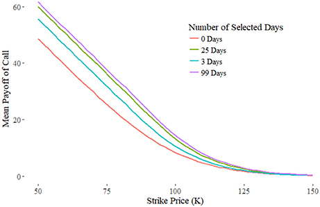
Figure 7. Amnesiac Call Payoff with fixed strike.

FIGURE 8

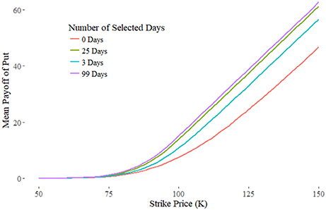
Figure 8. Amnesiac Put Payoff with fixed strike.

When the number of monitoring periods is equal to 0, then the maximum is simply the last stock price at time N. Thus, the payoff is the final stock price minus the strike.The shape of this curve for selecting n periods is therefore a simple, vertical translation. Through these observations, we have demonstrated the bounds for the amnesiac option as shown in Figure 9. It is bounded by the standard lookback from above, and the vanilla European options from below.

FIGURE 9

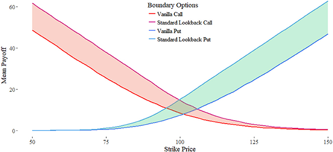
Figure 9. The payoffs of the upper and lower bounds for the call and put respectively. The area between demonstrate the customizable area of the instrument payoff.

3.3. Random vs. Equal Monitoring

One of the most important questions this paper addresses is if the choice of period matters in the payoff. What we find is randomly choosing lookback periods yields a worse payoff than equally spacing the days to look back on, as shown in Figure 10. The differences are shown in Figures 11, 12.

FIGURE 10

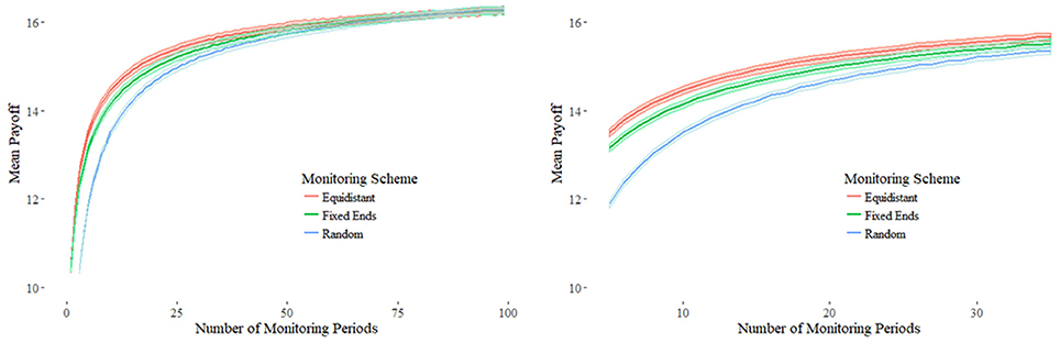
Figure 10. Equidistant Monitoring (red) yields higher payoffs than random monitoring with fixed endpoints (green) and true random monitoring (blue). Confidence intervals at 95% with 10000 simulations are shown.

FIGURE 11

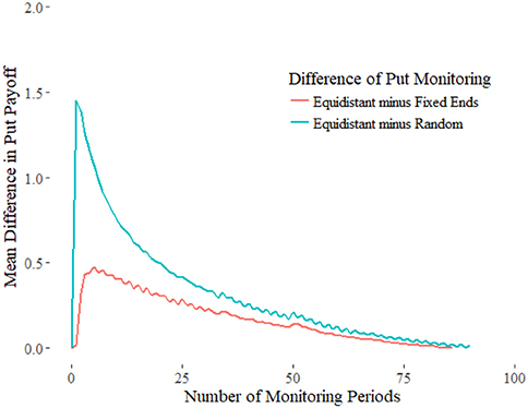
Figure 11. Put option difference between equidistant monitoring and random monitoring payoffs.

FIGURE 12

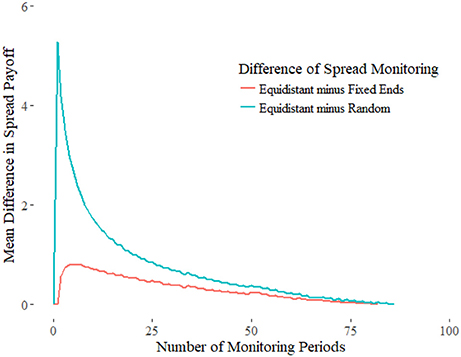
Figure 12. Spread option difference between equidistant monitoring and random monitoring payoffs.

There are two ways to monitoring randomly. We defined N equidistant points between time 0 and T, making it discrete. Suppose we are monitoring k points from the Gaussian Random walk. Under true random monitoring we would select k random points from the set of periods {0, 1, 2, …, N−1}. In contrast, the fixed-end random monitoring selects the first period n = 0 then randomly chooses k−1 periods from indices 1 through N−1. Since the price of an option increases with the duration of the contract, fixing the first and last period ensures an equal time length for comparison. For the true random monitoring, the time to maturity would be the minimum of index.

For illustration, suppose k = 2. For fixed-end random sampling the first period is chosen while the second can be any point between 1 and N−1. More simply, both endpoints are fixed, and we are choosing a point between the beginning and end. Numerical results in Figure 13 on average selection of the midpoint as more optimal. True random sampling produces weak payoffs due to shortened maturities. However, even when endpoints are always chosen to lookback on, the payoff for equidistant sampling is superior. Although this suggests the optimal strategy is to equally space the selected periods, this does not take into account sudden volatility swings from extreme, singular events.

FIGURE 13

Figure 13. Payoff for k = 2 with floating strike. The payoffs of always choosing the midpoint is greater than random sampling.

The intuition for this toy experiment can be explained as follows. Since both endpoints are fixed, we are only interested in choosing the point in-between. If the point chosen is less than or equal to S₀ or S_N, then the payoff is the same as the case of choosing one point, which is S₀. For the third point S_i to be of value it must satisfy S_i > S₀ and S_i > S_N. Suppose n is very close to the first index 0, then $S_n=S_0{e}^{ϵ}$ for ϵ that falls in the upper half of the Gaussian distribution defined in Equation (2). The difference between S₀ and S_n is thus small, and the payoff will be close to that of the case of just choosing the first point. On the other hand, suppose n is close to N. Then $S_N=S_n{e}^{ϵ}$. Since the payoff is just the difference between the max and final value, the payoff is diminished.

Simply put, given that the chosen point S_n is greater than S₀ and S_N, then choosing too close to the beginning means not giving enough distance for the maximum to rise, and choosing too close to the end means diminished payoff due to proximity with S_N. Intuitively, time value is then the explanatory factor that determines how much marginal payoff a selected period gives, where the value of a point is proportional to the time value associated with the distance between it and the closest adjacent lookback period.

We now demonstrate the above claim mathematically. For simplicity we fix the first period and denote j = k−1 as the number of lookback periods. Then let N denote the total number of equally spaced periods of the standard lookback with total time T, and let A be the set of selected periods. Define function γ that gives the minimum distance

$\begin{array}{cc}\gamma (i)=\min \{d(i,k)\forall k\in A,k\ne i\}& (13)\end{array}$

Then the totals of time value is given as

$\begin{array}{cc}\Gamma (A)={\displaystyle \sum _{i\in A}\gamma }(i)& (14)\end{array}$

where the value of Γ for equidistant sampling is $\frac{j}{j+1}$. We show this value is maximal.

Consider the base case of n = 1. If $i_0=\frac{N}{2}$ the only element in A₀, then $\Gamma (A_0)=\frac{N}{2}$. Compare to this to A₁ whose only element $i_1=\frac{N}{2}+ϵ$ for $ϵ\in {\mathbb{Z}}^{+},ϵ<\frac{N}{2}$. Since $d(0,i_1)>\frac{N}{2}$, then $d(i_1,N)=\frac{N}{2}-ϵ<\frac{N}{2}$. Thus $\Gamma (A_1)=\frac{N}{2}-ϵ<\Gamma (A_0)$. By symmetry, any i₁ greater or less than $\frac{N}{2}$ is worth less. Cases for larger j can be shown in a similar fashion by assuming the first point greater than $\frac{N}{j}$. Thus our claim that lookback period value is proportional to the time value of the next closest period remains true.

What this conclusion implies in real situation trading is that it would be inefficient to cluster lookback points around a presumed volatile event in order to capture a price extrema, even if volatility spikes seem certain, because the marginal value of each period chosen beyond the first in the locality diminishes rapidly due to the decreasing proximity of neighboring points. Prices are less likely to change a significant amount between two points in time the closer the two points in time are.

From the framework of analysis, suppose we sub-divide Geometric Brownian Motion into N subintervals defined by select indices. Then we are interested in the endpoints [i, i+1] as our monitoring dates. If these subintervals are of equal length, then the probability of the true maximum being captured is equal, since within the subinterval, the maximum is equally likely to fall on any point. Thus, the probability of the maximum being captured by the neighborhood around the endpoints diminish as subintervals get larger. The maximal neighborhoods are when endpoints are equally spaced.

This has been explored in the risk theory and queuing theory literature, which assumes expected maxima calculations on equidistant sampling. For further references consider papers by Janssen and Van Leeuwaarden [42, 43] on equidistant sampling of Brownian Motion and Gaussian Random Walks, and Alfi's work on exacting roughness in finite random walks [44]. Under equidistant sampling, the expected maximum shown using the Spitzer Identity which gives the joint distribution of partial sums and their maximal sums for a collection of random variables:

$\begin{array}{cc}𝔼\underset{n=0,\mathrm{...},N}{\max }B(\frac{n}{N})={\displaystyle \sum _{n=1}^N\frac{1}{n}}𝔼\max \{\frac{n}{N}\}& (15)\end{array}$

Now let the process X_n be defined as

$\begin{array}{cc}{X}_n={\displaystyle \sum _{i=1}^n{\delta }_{xi}}& (16)\end{array}$

After computation [44], the expected maximum value can be expressed as the following

$\begin{array}{cc}𝔼(M_k)=\underset{s\to 1}{\lim }\frac{𝔼(s^{M_k})-1}{\ln (s)}={\displaystyle \sum _{i=1}^k\frac{𝔼(|X_i|)}{2i}}& (17)\end{array}$

Adapting these results to Gaussian random walks with unequal steps may produce approximations for the payoff of lookbacks and other exotic options.

If the events of the world are analogous to random occurrences, then nonrandom selection of lookback periods is akin to event-based trading strategies. Specifically in regards to the amnesiac lookback option, such a strategy leads to lower payoffs. This conclusion implies that given general market efficiency, event-based period selection strategies of lookback periods should be unprofitable.

4. Discussion

These results can be immediately applied to pricing cryptocurrency. Under the Black-Scholes model, the implied volatility is usually calculated using the current market price of the option. However, because this is a new option being proposed, and since both futures and vanilla options are still new derivatives on the market, it is not possible at this time to even price them with rudimentary Monte-Carlo simulations.

Instead, we use the historical volatility as a proxy and use the 3-month treasury bond as the risk-free rate. Tables 4, 5 show the prices of amnesiac calls and puts based on historical data in a 3 and 2 month window, respectively. These are then shown as a ratio of the initial price in Figure 14. Data is taken from Coinmarketcap.

TABLE 4

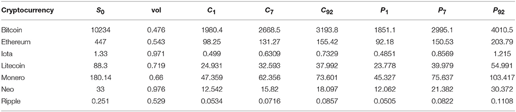
Table 4. Amnesiac call and put prices using historical volatility August 31, 2017 to November 30, 2017.

TABLE 5

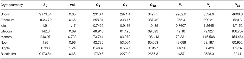
Table 5. Amnesiac call and put prices using historical volatility December 01, 2017 to February 01, 2018.

FIGURE 14

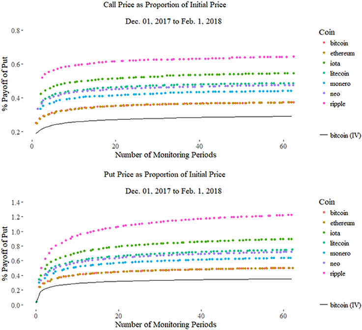
Figure 14. The prices of the calls and puts for a given Cryptocurrency priced with risk-free rate 0.0125. The pricing with Implied Volatility is lower than any coin using historical volatility.

The last row in Table 5 shows a Bitcoin amnesiac option priced at the implied volatility of Bitcoin calls in December. Interestingly, it is less than the minimum volatility of Bitcoin itself. When the implied volatility is less than historic volatility, this indicates that market sentiment benefits option buyers. In other words, the market expects lower volatility in the future, and as a result, using historical volatility as a proxy is prone to overpricing.

To verify this is what we expect, we observe a linear correlation between the price of the amnesiac lookback and its volatility, yielding a correlation coefficient is r² = 0.99. An interesting point is the difference in shape between the call and the put curves. As seen in Figure 14, the put curves slower than the call, due to the right vs. left tail of the lognormal distribution, especially when volatility is high in the case of ripple. This means that the amnesiac put may be useful if a trader anticipates a down market without needing to worry when to sell, while enjoying a greater range of values to choose from due to the slower convergence to the standard lookback option.

One can conceive of using Algorithm 1 to price an option, particularly for Ethereum which was developed for Smart Contracts via the Ethereum Virtual Machine (EVM). The scripting language it uses is very expressive and Turing complete, and the EVM acts as a distributed computer that executes commands based on the resource gas. Smart contracts thus become a good way to buy contracts that previously only existed in the OTC market. In this case, a transaction function transfers Ether to the writers account at the time of purchase. At the time of maturity, if the option is exercised, the smart contract executes the necessary transactions as determined by the option automatically. The buyer sends in a selection of monitoring periods A, then the input parameter could be the number of periods which is used to generate a subset of pseudorandom monitoring periods, or direct simulation of the selected periods. The latter produces a more accurate price but is also computationally more expensive and as a result, raises the transaction fees of the smart contract. The choice becomes a question of cost vs. profit, and once statistical distributions on people's preferences of monitoring periods are collected, the pricing can be made even more accurate at lower computational costs.

5. Conclusion

Lookback options are immensely useful instruments for the use of hedging against risks associated with high volatility and notably effective at canceling investor regret as well. Although the literature has explored lookback options and many concepts of the partial lookback, previous work has mainly involved lookbacks with continuous monitoring, and equidistant lookback period selection. We suggest the use and exploration of a new form of partial lookback, the amnesiac lookback option, that can look back upon any discretely selected period prior to expiration.

We discuss the practical applications that amnesiac lookback options may have in the trading of cryptocurrencies such as Bitcoin and especially Ethereum. The cryptocurrency market has been defined by its high volatility trading and plethora of exogenous shocks that regularly disrupt the market. In such a high risk and speculative market, it is imperative that investors have some way of mitigating their risks and exposures. In this realm, lookback options are a simple and effective way to do so, while amnesiac lookback options allow an investor to fully customize the amount of risk he is willing to take on or forego by adjusting the number of lookback periods, and potentially where to place them, as shown in Figure 1. This is particularly true for put options under high volatility. Past studies have also found long memory in Bitcoin returns and return volatility, which path-dependent options such as the amnesiac lookback are able to correct by closing arbitrage opportunities, if traded on rationally. This opportunity is greatly enhanced by Smart Contracts, which decentralizes and automates highly customizable derivatives like path-dependent options.

Using Monte Carlo simulations under Black-Scholes assumptions, we find the Hill Function to be a suitable model for pricing the payoffs of the amnesiac lookback option. We also determine the bounds of the amnesiac lookback consistent with prior results on partial lookbacks, that is the standard lookback from above, and the corresponding vanilla European option (call or put) from below.

Our work additionally discusses the merits of equal spacing vs. random sampling of lookback periods. In this regard, we find that equally spaced lookback periods yield the greatest payoffs under Black-Scholes assumptions. Since the formula for modified trees and lattice methods produce analytic results for equidistant sampling, and equidistant sampling is a strict upper bound for random sampling, we can conclude that if days are not chosen equally then the instrument will be prone to being overpriced. More importantly, our results are more realistic and related to the designated function of these options in actual markets than some previous works.

The fact that how periods are selected affect the pricing suggest multiple paths of further inquiry. Since this is phenomenon under Black-Scholes assumptions, different models such as introducing stochastic volatility and Lévy processes may produce different results. Tying this to real commodities, statistical analysis of Cryptocurrency data can benchmark the efficiency of such an option. Simulating extreme, volatile events within the context of the Gaussian random walk would bridge the empirical and axiomatic formulations, and is ultimately the purpose of having a choice in monitoring periods. Understanding period selection strategies will yield new perspectives of using path-dependent options for hedging risk, and expand trading strategies with the growth of novel and volatile blockchain commodities.

Author Contributions

H-CC wrote the code for the numerical simulation, data processing, and the mathematical finance literature review. KL contributed economic analyses, interpretation, literature review and extension to cryptocurrencies. Both contributed to the conception and design of the option's amnesiac feature, interpretation of results, and general authorship the paper.

Funding

Funding for this research was provided by the Jack Byrne Scholar Fund at the Department of Mathematics, Dartmouth College. Open access article fees were provided by the Dartmouth Open-Access Publication Equity Fund.

Conflict of Interest Statement

The authors declare that the research was conducted in the absence of any commercial or financial relationships that could be construed as a potential conflict of interest.

Acknowledgments

We'd like to thank Seema Nanda for proof-reading and overall suggestions, Feng Fu, Sergi Elizalde and Peter Winkler at the Department of Mathematics, Dartmouth College for their mathematical suggestions, Jennifer Kuo for statistical consulting and Jonathan Meng for web scraping consultation.

References

1. Shreve SE. Stochastic Calculus for Finance I: The Binomial Asset Model. Vol. 11. New York, NY: Springer Science & Business Media (2004).

Google Scholar

2. Goldman MB, Sosin HB, Gatto MA. Path dependent options:“Buy at the low, sell at the high”. J Finan. (1979) 34:1111–27.

Google Scholar

3. Goldman MB, Sosin HB, Shepp LA. On contingent claims that insure ex-post optimal stock market timing. J Finan. (1979) 34:401–13. doi: 10.1111/j.1540-6261.1979.tb02102.x

CrossRef Full Text | Google Scholar

4. Schwert GW. Anomalies and market efficiency. Handb Econ Finan. (2003) 1:939–74. doi: 10.1016/S1574-0102(03)01024-0

CrossRef Full Text | Google Scholar

5. Kat HM, Heynen RC. Selective memory. Risk (1994) 7:73–6.

Google Scholar

6. Conze A, Viswanathan. Path dependent options: the case of lookback options. J Finan. (1991) 46:1893–907. doi: 10.1111/j.1540-6261.1991.tb04648.x

CrossRef Full Text | Google Scholar

7. Buchen P, Konstandatos O. A new method of pricing lookback options. Math Finan. (2005) 15:245–59. doi: 10.1111/j.0960-1627.2005.00219.x

CrossRef Full Text | Google Scholar

8. Carrick J. Bitcoin as a complement to emerging market currencies. Emerg Markets Finan Trade (2016) 52:2321–34. doi: 10.1080/1540496X.2016.1193002

CrossRef Full Text | Google Scholar

9. The Guardian. Don't Dismiss Bankers' Predictions of a Bitcoin Bubble – They Should Know. Guardian News Media (2017). Available online at: https://www.theguardian.com/business/2017/sep/17/jamie-dimon-bitcoin-bubble-he-would-know-banking

10. Buy Bitcoin Worldwide. The Bitcoin Volatility Index. Available online at: https://www.buybitcoinworldwide.com/volatility-index/

11. Bariviera AF, Basgall MJ, Hasperué W, Naiouf M. Some stylized facts of the Bitcoin market. Phys A (2017) 484:82–90. doi: 10.1016/j.physa.2017.04.159

CrossRef Full Text | Google Scholar

12. Urquhart A. Price clustering in Bitcoin. Econ Lett. (2017) 159:145–8. doi: 10.1016/j.econlet.2017.07.035

CrossRef Full Text | Google Scholar

13. Times TE. Bitcoins Lose Lustre in the Face of Flak (2017). Available online at: http://economictimes.indiatimes.com/wealth/personal-finance-news/bitcoins-lose-lustre-in-the-face-of-flak/articleshow/60709423.cms

14. Bouri E, Gupta R, Tiwari AK, Roubaud D. Does Bitcoin hedge global uncertainty? Evidence from wavelet-based quantile-in-quantile regressions. Finan Res Lett. (2017) 23:87–95. doi: 10.1016/j.frl.2017.02.009

CrossRef Full Text | Google Scholar

15. Bouri E, Molnár P, Azzi G, Roubaud D, Hagfors LI. On the hedge and safe haven properties of Bitcoin: is it really more than a diversifier? Finan Res Lett. (2017) 20:192–8. doi: 10.1016/j.frl.2016.09.025

CrossRef Full Text | Google Scholar

16. Russo C. Bitcoin Options Will Be Available This Fall. Bloomberg (2017). Available online at: https://www.bloomberg.com/news/articles/2017-07-24/bitcoin-options-to-become-available-in-fall-after-cftc-approval

17. U S Commodity Futures Trading Commision. CFTC Statement on Self-Certification of Bitcoin Products by CME, CFE and Cantor Exchange. CFTC (2017). Available online at: https://www.cftc.gov/PressRoom/PressReleases/pr7654-17

18. Roberts D. Why Nasdaq, CME, CBOE All Want in on Bitcoin Futures. Yahoo! (2017). Available online at: https://finance.yahoo.com/news/nasdaq-cme-cboe-want-bitcoin-futures-183256191.html

19. Szabo N. Smart contracts: building blocks for digital markets. In: EXTROPY: The Journal of Transhumanist Thought. Marina Del Rey, CA (1996).

20. Szabo N. The idea of smart contracts. In: Nick Szabo's Papers and Concise Tutorials (1997). Available online at: http://www.fon.hum.uva.nl/rob/Courses/InformationInSpeech/CDROM/Literature/LOTwinterschool2006/szabo.best.vwh.net/idea.html

21. Buterin V. A next-generation smart contract and decentralized application platform. In: White Paper (2014). Available online at: https://www.weusecoins.com/assets/pdf/library/Ethereum_white_paper-a_next_generation_smart_contract_and_decentralized_application_platform-vitalik-buterin.pdf

Google Scholar

22. Wright A, De Filippi P. Decentralized Blockchain Technology and the Rise of Lex Cryptographia (March 10, 2015). doi: 10.2139/ssrn.2580664

CrossRef Full Text

23. Omohundro S. Cryptocurrencies, smart contracts, and artificial intelligence. AI Matt. (2014) 1:19–21. doi: 10.1145/2685328.2685334

CrossRef Full Text | Google Scholar

24. De N. Smart Contracts Now Recognized Under Tennessee Law (2018). Available online at: https://www.coindesk.com/blockchain-bill-becomes-law-tennessee/

25. Peters G, Panayi E, Chapelle A. Trends in cryptocurrencies and blockchain technologies: a monetary theory and regulation perspective. J. Financ. Perspect. (2015) 3. Available online at: https://ssrn.com/abstract=3084011

Google Scholar

26. Musiela M, Rutkowski M. Martingale Methods in Financial Modelling, volume 36 of Applications of Mathematics: Stochastic Modelling and Applied Probability. New York, NY: Springer (1997).

27. Kat HM, Heynen RC. Lookback options with discrete and partial monitoring of the underlying price. Appl Math Finan. (1995) 2:273–84. Available online at: http://www.tandfonline.com/doi/abs/10.1080/13504869500000014

Google Scholar

28. Babbs S. Binomial valuation of lookback options. J Econ Dyn Cont. (2000) 24:1499–525. doi: 10.1016/S0165-1889(99)00085-8

CrossRef Full Text | Google Scholar

29. Cheuk TH, Vorst TC. Currency lookback options and observation frequency: a binomial approach. J Int Money Finan. (1997) 16:173–87. doi: 10.1016/S0261-5606(96)00052-6

CrossRef Full Text | Google Scholar

30. Leung KS. An analytic pricing formula for lookback options under stochastic volatility. Appl Math Lett. (2013) 26:145–9. doi: 10.1016/j.aml.2012.07.008

CrossRef Full Text | Google Scholar

31. Dia EHA, Lamberton D. Connecting discrete and continuous lookback or hindsight options in exponential Lévy models. Adv Appl Probabil. (2011) 43:1136–65. doi: 10.1239/aap/1324045702

CrossRef Full Text | Google Scholar

32. Cox JC, Ross SA, Rubinstein M. Option pricing: a simplified approach. J Finan Econ. (1979) 7:229–63. doi: 10.1016/0304-405X(79)90015-1

CrossRef Full Text | Google Scholar

33. Hull JC, White AD. Efficient procedures for valuing European and American path-dependent options. J Derivat. (1993) 1:21–31. doi: 10.3905/jod.1993.407869

CrossRef Full Text

34. Aitsahlia F, Le Lai T. Random walk duality and the valuation of discrete lookback options. Appl Math Finan. (1998) 5:227–40. doi: 10.1080/135048698334655

CrossRef Full Text | Google Scholar

35. Petrella G, Kou S. Numerical pricing of discrete barrier and lookback options via Laplace transforms. J Comput Finan. (2004) 8:1–38. doi: 10.21314/JCF.2004.114

CrossRef Full Text | Google Scholar

36. Broadie M, Glasserman P, Kou SG. Connecting discrete and continuous path-dependent options. Finan Stochast. (1999) 3:55–82. doi: 10.1007/s007800050052

CrossRef Full Text | Google Scholar

37. Fusai G, Germano G, Marazzina D. Spitzer identity, Wiener-Hopf factorization and pricing of discretely monitored exotic options. Eur J Operat Res. (2016) 251:124–34. doi: 10.1016/j.ejor.2015.11.027

CrossRef Full Text | Google Scholar

38. Boyarchenko S, Levendorski S. Efficient Laplace inversion, Wiener-Hopf factorization and pricing lookbacks. Int J Theor Appl Finan. (2013) 16:1350011. doi: 10.1142/S0219024913500118

CrossRef Full Text | Google Scholar

39. Hieber P. Pricing exotic options in a regime switching economy: a Fourier transform method. Rev Derivat Res. (2017) 1–22. doi: 10.1007/s11147-017-9139-1

CrossRef Full Text | Google Scholar

40. Feng L, Linetsky V. Computing exponential moments of the discrete maximum of a Lévy process and lookback options. Finan Stochast. (2009) 13:501–29. doi: 10.1007/s00780-009-0096-x

CrossRef Full Text | Google Scholar

41. Dai TS, Liu LM, Lyuu YD. Linear-time option pricing algorithms by combinatorics. Comput Math Appl. (2008) 55:2142–57. doi: 10.1016/j.camwa.2007.08.046

CrossRef Full Text | Google Scholar

42. Janssen AJEM, Van Leeuwaarden J. Cumulants of the maximum of the Gaussian random walk. Stochast Process Their Appl. (2007) 117:1928–59. doi: 10.1016/j.spa.2007.03.006

CrossRef Full Text | Google Scholar

43. Janssen AJEM, Van Leeuwaarden JSH. On Lerch's transcendent and the Gaussian random walk. Ann Appl Probabil. (2007) 17:421–39. doi: 10.1214/105051606000000781

CrossRef Full Text | Google Scholar

44. Alfi V, Coccetti F, Marotta M, Petri A, Pietronero L. Exact results for the roughness of a finite size random walk. Phys A (2006) 370:127–31. doi: 10.1016/j.physa.2006.04.020

CrossRef Full Text | Google Scholar