Brownian Forgery of Statistical Dependences

1. Introduction

The modern theory of Brownian motion provides an exceptionally successful example of how physical models can have far-reaching consequences beyond their initial field of development. Since its introduction as a model of particle diffusion, Brownian motion has indeed enabled the description of a variety of phenomena in cell biology, neuroscience, engineering, and finance [1]. Its mathematical formulation, based on the Wiener measure, also represents a fundamental prototype of continuous-time stochastic process and serves as powerful tool in probability and statistics [2, 3]. Following a similar vein, we develop in this note a new way of applying Brownian motion to the characterization of statistical independence.

Our connection between Brownian motion and independence is motivated by recent developments in statistics, more specifically the unexpected coincidence of two different-looking dependence measures: distance covariance, which characterizes independence fully thanks to its built-in sensitivity to all possible relationships between two random variables [4], and Brownian covariance, a version of covariance that involves nonlinearities randomly generated by a Brownian process [5]. Their equivalence provides a realization of the aforementioned connection, albeit in a somewhat indirect way that conceals its naturalness. Our goal is to explicit how Brownian motion can reveal statistical independence by relying directly on the geometry of its sample paths.

The brute force method to establish the dependence or independence of two real-valued random variables X and Y consists in examining all potential relations between them. More formally, it is sufficient to measure the covariances cov[f(X), g(Y)] associated with transformations f, g that are bounded and continuous (see, e.g., Theorem 10.1 Jacod and Protter [6]). The question pursued here is whether using sample paths of Brownian motion in place of bounded continuous functions also allows to characterize independence, and we shall demonstrate that the answer is yes. In a nutshell, the statistical fluctuations of Brownian paths B, B′ enable the stochastic covariance index cov[B(X),B′(Y)] to probe arbitrary dependences between the random variables X and Y.

Our strategy to realize this idea consists in establishing that, given any pair f, g of bounded continuous functions and any level of accuracy, the covariance cov[f(X), g(Y)] can be approximated generically by cov[B(X),B′(Y)]. Crucially, the notion of genericity used here refers to the fact that the probability of picking paths B, B′ fulfilling this approximation is nonzero, which ensures that an appropriate selection of stochastic covariance can be achieved by finite sampling of Brownian motion. This core result of the paper will be referred to as the forgery of statistical dependences, in analogy with Levy's classical forgery theorem [2].

Actually Levy's remarkable theorem, which states that any continuous function can be approximated on a finite interval by generic Brownian paths, provides an obvious starting point of our analysis. Indeed, it stands to reason that if the paths B and B′ approach the functions f and g, respectively, then cov[B(X),B′(Y)] should approach cov[f(X), g(Y)] as well. A technical difficulty, however, lies with the restriction to finite intervals since the random variables X and Y may be unbounded. Although it turns out that intervals can not be prolonged as such without ruining genericity, we shall describe first a suitable extension of Levy's forgery that holds on infinite domains. Our forgery of statistical dependences will then follow.

From a practical standpoint, using Brownian motion to establish independence turns out to be advantageous. Indeed, exploring all bounded continuous transformations exhaustively is realistically impossible. (This practical difficulty motivates the use of reproducing kernel Hilbert spaces, see e.g., Gretton and Györfi [7] for a review). Generating all possible realizations of Brownian motion obviously poses the same problem, but this unwieldy task can be bypassed by averaging directly over sample paths. In this way, and quite amazingly, the measurement of an uncountable infinity of covariance indices can be replaced by a single functional integral. We shall discuss how this idea leads back to the concept of Brownian covariance and how the forgery of statistical dependences clarifies the way it does characterize independence, without reference to the equivalence with distance covariance. Brownian covariance represents a very promising tool for modern data analysis [8, 9] but appears to be still scarcely used in applications (with seminal exceptions for nonlinear time series [10] or brain connectomics [11]). Our approach based on random paths is both physically grounded and mathematically rigorous, so we believe that it may help further disseminate this method and establish it as a standard tool of statistics.

2. Main Results

Here we motivate and describe our main results, with sufficient precision to provide a self-contained presentation of the ideas introduced above while avoiding technical details, which are then developed in the dedicated section 3. We also use here assumptions that are slightly stronger than is necessary, and some generalizations are relegated to the Supplementary Material S1.

2.1. Extension of Levy's Forgery

Imagine recording the movement of a free Brownian particle in a very large number of trials. In essence, Levy's forgery ensures that one of these traces will follow closely a predefined test trajectory, at least for some time. To formulate this more precisely, let us focus for definiteness on standard Brownian motion B, whose initial value is set to B(0) = 0 and variance at time t is normalized to 〈B(t)²〉 = |t|. We fix a real-valued continuous function f with f(0) = 0 (the test trajectory) and consider the uniform approximation event that a Brownian path B fits f tightly up to a constant distance δ > 0 on the time interval [−T, T],

$\begin{array}{cc}{{U}}_{f,\delta ,T}=\{|\text{B}(t)-f(t)|<\delta ,\forall |t|\le T\}.& (1)\end{array}$

Levy's forgery theorem states that this event is generic, i.e., it occurs with probability P(${U}$_f,δ,T) > 0 (see Chapter 1, Theorem 38 in [2]). This result requires both the randomness and the continuity of Brownian motion. Neither deterministic processes nor white noises satisfy this property.

In all trials though, the particle will eventually drift away to infinity and thus deviate from any bounded test trajectory. Indeed, let us further assume that the function f is bounded and examine what happens when T → ∞. If the limit event ${U}$_f,δ,∞ = ⋂_{T > 0} ${U}$_f,δ,T occurs, the path B must be bounded too since the particle is forever trapped in a finite-size neighborhood of the test trajectory. However Brownian motion is almost surely (a.s.) unbounded at long times [2], so that P(${U}$_f,δ,∞) = 0. Hence Levy's forgery theorem does not work on infinite time domains.

To accommodate this asymptotic behavior, we should thus allow the particle to diverge from the test trajectory, at least in a controlled way. Let us recall that the escape to infinity is a.s. slower for Brownian motion than for any movement at constant velocity (which is one way to state the law of large numbers [2]). This suggests adjoining to event (1) the loose approximation event

$\begin{array}{cc}{ℰ}_{f,v,T}=\{|\text{B}(t)-f(t)|<v|t|,\forall |t|\ge T\}& (2)\end{array}$

whereby the particle is confined to a neighborhood of the test trajectory that expands at finite speed v > 0.

Asymptotic forgery theorem. Let f be bounded and continuous, and v, T > 0. Then P(${E}$_{f, v, T}) > 0.

An elegant, albeit slightly abstract, proof rests on a short/long time duality between the classes of events (1) and (2), which maps Levy's forgery and this asymptotic version onto each other (see section 3.1). For a more concrete approach, let us focus on the large T limit that will be used to study statistical dependences. Since the path B(t) and the neighborhood size v|t| both diverge, the bounded term f(t) can be neglected in Equation (2) and the event ${E}$_f,v,T thus merely requires not to outrun deterministic particles moving at speed v. The asymptotic forgery thus reduces to the law of large numbers, which ensures that P(${E}$_f,v,T) is close to one for all T ≫ 1. This probability decreases continuously as T is lowered [since the defining condition in Equation (2) becomes stricter] but does not drop to zero until T = 0 is reached. This line of reasoning can be completed and also generalized to allow slower expansions (see Supplementary Material S1).

We now combine Levy's forgery and the asymptotic version to obtain an extension valid at all timescales. Specifically, let us examine the joint approximation event

$\begin{array}{cc}{{J}}_{f,\delta ,T}={{U}}_{f,\delta ,T}{\displaystyle \cap {ℰ}_{f,v,T}}\text{ with }v=\delta /T.& (3)\end{array}$

In words, the particle is constrained to follow closely the test trajectory for some time but is allowed afterwards to deviate slowly from it (Figure 1).

FIGURE 1

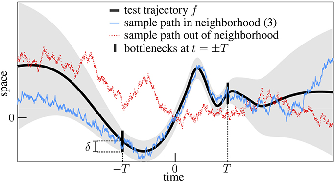
Figure 1. Extended forgery of continuous functions. This example depicts a test trajectory (smooth curve), its allowed neighborhood (shaded area) and two sample paths, one (solid random walk) illustrating the generic event (3) and the other (dotted random walk), the fact that arbitrary paths have low chances to enter the expanding neighborhoods through the bottlenecks.

Extended forgery theorem. Let f be bounded and continuous with f(0) = 0, and δ, T > 0. Then P(${J}$_f,δ,T) > 0.

This result relies on the suitable integration of a “local” version of the theorem (see section 3.2), but it can also be understood rather intuitively as follows. Imagine for a moment that the events (1) and (2) were independent. Their joint probability would merely be equal to the product of their marginal probabilities, which are positive by Levy's forgery and the asymptotic forgery, and genericity would then follow. Actually they do interact because the associated neighborhoods are connected through the narrow bottlenecks at t = ±T (Figure 1) but this should only increase their joint probability, i.e.,

$\begin{array}{cc}P({{J}}_{f,\delta ,T})>P({{U}}_{f,\delta ,T})P({ℰ}_{f,v,T}).& (4)\end{array}$

The reason lies in the temporal continuity of Brownian motion. A particle staying in the uniform neighborhood while |t| ≤ T necessarily passes through the bottlenecks, and is thus more likely to remain within the expanding neighborhood than arbitrary particles, which have low chances to even meet the bottlenecks (Figure 1). In other words, the proportion P(${J}$_f,δ,T)/P(${U}$_f,δ,T) of sample paths B ∈ ${E}$_f,v,T among all those sample paths B ∈ ${U}$_f,δ,T should be larger than the unconstrained probability P(${E}$_f,v,T), hence the bound (4).

2.2. Forgery of Statistical Dependences

We now turn to the analysis of statistical relations using Brownian motion. Let us fix two random variables X,Y and a pair of bounded test trajectories f, g. Consider the covariance approximation event

$\begin{array}{cc}{{C}}_{\text{X},\text{Y},f,g,\epsilon }=\{|\text{cov}[\text{B}(\text{X}),{\text{B}}^{\prime }(\text{Y})]-\text{cov}[f(\text{X}),g(\text{Y})]|<\epsilon \}& (5)\end{array}$

whereby the stochastic covariance cov[B(X),B′(Y)], built by picking independently two sample paths B,B′, coincides with the test covariance cov[f(X), g(Y)] up to a small error ε > 0 (Figure 2). We argue that this event is generic too.

FIGURE 2

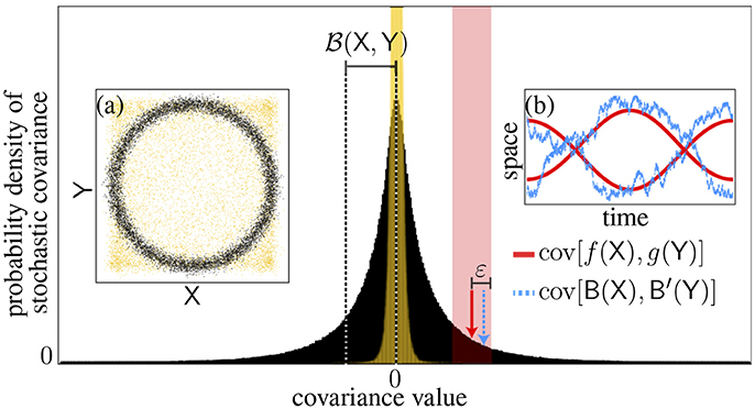
Figure 2. Forgery of statistical dependences. The distribution of the stochastic covariance (black histogram) and its standard deviation [${B}$(X,Y)] are shown for simulated dependent random variables [n = 10⁴ black dots, Insert (a)] as well as a test covariance (plain arrow) and a sample (dotted arrow) falling within the allowed error (shaded area). Insert (b) shows the associated functions. The case of independent variables is superimposed (yellow) for comparative purposes.

The first step is to ensure that the set (5) is measurable so that its probability is meaningful. Physically, this technical issue is rooted once again in the escape of Brownian particles to infinity. The stochastic covariance can be expressed as a difference of two averages 〈B(X)B′(Y)〉 and 〈B(X)〉〈B′(Y)〉 (computed at fixed sample paths) involving the coordinates B(t),B′(t′) at random moments t = X, t′ = Y. If long times and thus large coordinates are sampled too often, the two terms may diverge and lead to an ill-defined covariance, i.e., ∞ − ∞. To avoid this situation, we should therefore assume that asymptotic values of X and Y are unlikely enough. Actually we shall adopt hereafter the sufficient condition that X,Y are L₂, i.e., they have finite mean and variance. (See Supplementary Material S2 for a derivation of measurability).

Forgery theorem of statistical dependences. Let X,Y be L₂ random variables, f, g be bounded and continuous, and ε > 0. Then P(${C}$_{X,Y, f, g, ε}) > 0.

The idea is that one way of realizing the event (5) is to pick sample paths B ∈ ${J}$_f,δ,T, ${\text{B}}^{\prime }\in {{J}}_{g,\delta ,T}$ that fit the test trajectories f, g tightly (δ ≪ 1) over a long time period (T ≫ 1), see Figure 2b. Indeed, as shown below, we have then

$\begin{array}{cc}\text{cov}[\text{B}(\text{X}),{\text{B}}^{\prime }(\text{Y})]-\text{cov}[f(\text{X}),g(\text{Y})]={O}(\delta )+{O}(v)& (6)\end{array}$

with v = δ/T. This rough estimate explains why the event (5) must occur whenever δ and v are small enough [see section 3.3, in particular Equations (27) and (28) for a more precise error bound and the nested forgery lemma (29) for a full derivation]. In turn, the extended forgery ensures the genericity of this selection of sample paths B,B′ and thus of the event ${C}$_{X,Y, f, g, ε} as well [the necessary condition f(0) = g(0) = 0 can indeed be assumed without loss of generality, see Equation (31) in section 3.3].

To understand Equation (6), imagine first that the random times were bounded with |X|, |Y| ≤ T. Then B(X),B′(Y) differ from f(X), g(Y) by less than δ for all times X,Y (Equation 1) so the covariance error must be ${O}$(δ) at most. Now for unbounded random times the distance between sample paths and test trajectories may exceed δ and must actually diverge at long times, which could have led to an infinitely large covariance error if not for the fact that the occurence of |X| ≥ T or |Y| ≥ T is very unlikely. So the fit divergence v|t| (see Equation 2) is counterbalanced within averages by the fast decay of long times probability [e.g., P(|X| ≥ |t|) ≤ 〈X²〉/t²]. The contribution of |X| ≥ T or |Y| ≥ T to the covariance error is thus finite and scales as ${O}$(v), which leads to Equation (6).

This forgery theorem allows us to probe enough possible relationships to establish statistical dependence or independence, as we explain now. Consider the two probability densities of stochastic covariance shown in Figure 2, which were generated using simulations differing only by the presence or absence of coupling between X and Y. The distribution appears significantly wider for the dependent variables, so this suggests that width is the key indicator of a relation. Actually, for the independent variables the narrow peak observed reflects an underlying Dirac delta function (its nonzero width in Figure 2 is due to finite sampling errors in the covariance estimates). Indeed the vanishing of all stochastic covariances is a necessary condition of independence. The impossibility of sampling nonzero values also turns out to be sufficient.

Brownian independence test. Two L₂ random variables X,Y are independent iff cov[B(X),B′(Y)] = 0 a.s.

To prove sufficiency, we show that the hypothesis cov[B(X),B′(Y)] = 0 a.s. implies that all test covariances vanish, which is equivalent to the independence of X and Y (Theorem 10.1 Jacod and Protter [6]). This can be understood concretely using the following thought experiment. Imagine that cov[f(X), g(Y)] ≠ 0 for some pair of test trajectories f, g and let us fix, say, ε = |cov[f(X), g(Y)]|/4 (as in Figure 2). We then generate sequentially samples of stochastic covariance until the approximation event ${C}$_{X,Y, f, g, ε} (Equation 5, shaded area in Figure 2) occurs. The forgery of statistical dependences ensures that this sequence stops eventually and our choice of ε, that the last covariance sample is nonzero. However this contradicts our hypothesis, which imposes that all trials result in vanishing covariance (see also section 3.4 for a set-theoretic argument).

Figure 2 suggests a straightforward manner to implement the Brownian independence test in practice. The sample distribution of the stochastic covariance cov[B(X),B′(Y)] can be generated by drawing a large number of sample paths B,B′, which can be approximated numerically via random walks (black histogram in Figure 2). Likewise, a null distribution can be built under the hypothesis of independence, e.g., by accompanying each walk simulation with a random permutation of the sample orderings within X and Y so as to break any dependency, hence leading to a finite-sample version of the Dirac delta (yellow histogram in Figure 2). These two distributions can then be compared statistically using, e.g., a Kolmogorov-Smirnov test. Actually, it is sufficient to focus on a comparison of their variances since width is the key parameter here. As it turns out, this provides a more efficient implementation because it is possible to integrate out B,B′ analytically in the variance statistic (i.e., all sample paths are probed exhaustively without the need of random walk simulations). This idea leads back to the notion of Brownian covariance.

2.3. Brownian Covariance Revisited

The forgery of statistical dependences provides an alternative approach to the theory of Brownian covariance, hereafter denoted ${B}$(X,Y). This dependence index emerges naturally in our context as the root mean square (r.m.s.) of the stochastic covariance (or equivalently its standard deviation since the mean 〈cov[B(X),B′(Y)]〉 vanishes identically by symmetry B↔−B, see also Figure 2). Thus

$\begin{array}{cc}\text{B}{(\text{X},\text{Y})}^2=\langle \text{cov}{[\text{B}(\text{X}),{\text{B}}^{\prime }(\text{Y})]}^2\rangle ,& (7)\end{array}$

which is only a slight reformulation of the definition in Székely GJ and Rizzo [5]. For L₂ random variables X,Y, the quadratic Gaussian functional integrals over the sample paths B,B′ can be computed analytically and the result reduces to distance covariance, so ${B}$(X,Y) inherits all its properties [5]. Alternatively, we argue here that the central results of the theory follow in a natural manner from Equation (7).

The first key property is that X,Y are independent iff ${B}$(X,Y) = 0. This mirrors directly the Brownian independence test since the r.m.s. (7) measures precisely the deviations of stochastic covariance from zero. This argument thus replaces the formal manipulations on the regularized singular integrals that underlie the theory of distance covariance [4]. Furthermore the forgery of statistical dependences clarifies how this works physically: Brownian motion fluctuates enough to make the functional integral (7) probe all the possible test covariances between X and Y.

The second key aspect is the straightforward sample estimation of ${B}$(X,Y) using a parameter-free, algebraic formula. This is an important practical advantage over other dependency measures such as, e.g., mutual information [12]. Instead of relying on the sample formula of distance covariance [4, 5], Equation (7) prompts us to estimate the stochastic covariance (or rather, its square) before averaging over the Brownian paths. So, given n joint samples X_i,Y_i (i = 1, …, n) of X,Y and an expression for their sample covariance ${\widehat{\mathrm{\text{cov}}}}_n$, the functional integral

$\begin{array}{cc}{\widehat{\text{B}}}_n{(\text{X},\text{Y})}^2={\langle {\widehat{\text{cov}}}_n{[\text{B}(\text{X}),{\text{B}}^{\prime }(\text{Y})]}^2\rangle }_{\text{samples }{\text{X}}_{\text{1}},{\text{Y}}_{\text{1}},\dots ,{\text{X}}_n,{\text{Y}}_n\text{ fixed}}& (8)\end{array}$

determines an estimator ${\hat{{B}}}_n(\text{X},\text{Y})$ of Brownian covariance. If X,Y are L₂ random variables, this procedure allows to build the estimation theory of Brownian (and thus, distance) covariance from that of the elementary covariance. For instance, the rather intricate algebraic formula for the unbiased sample distance covariance [13, 14] is recovered by using, quite naturally from Equations (7) and (8), an unbiased estimator ${\widehat{\mathrm{\text{cov}}}}_n{\left[·,·\right]}^2$ of the covariance squared (see section 3.5 for explicit expressions of these estimators and a derivation of this statement). The unbiasedness property $\langle {\widehat{\mathrm{\text{cov}}}}_n{\left[·,·\right]}^2\rangle =\mathrm{\text{cov}}{\left[·,·\right]}^2$ is then automatically transferred to the corresponding estimator (8), i.e.,

$\begin{array}{cc}\langle {\widehat{{B}}}_n{(\text{X},\text{Y})}^2\rangle ={B}{(\text{X},\text{Y})}^2,& (9)\end{array}$

because the L₂ convergence hypothesis is sufficient to ensure that averaging over the samples X_i,Y_i commutes with the functional integration over the Brownian paths B,B′.

Coming back to the implementation of the Brownian independence test, once an estimator ${\hat{{B}}}_n(\text{X},\text{Y})$ is found, its null distribution under the hypothesis of independence should be derived for formal statistical assessment. This may be done using large n approximations to obtain parametrically the asymptotic distribution or nonparametric methods also valid at small n (such as sample ordering permutations, as suggested above). Asymptotic tests are derived explicitly in Székely et al. [4], Székely and Rizzo [5, 13], where both parametric and nonparametric approaches are also illustrated on examples motivating the usefulness of this nonlinear correlation index in data analysis (including comparisons to linear correlation tests and assessments of statistical power).

It is noteworthy that our construction of Brownian covariance and its estimator can be generalized by formally replacing the Brownian paths B,B′ with other stochastic processes or fields (in which case we may consider multivariate variables X,Y). This determines a simple rule to engineer a wide array of dependence measures via functional integrals, and opens the question of what processes allow to characterize independence. Our approach relied on the ability to probe generically all possible test covariances but, critically, the class of processes satisfying a forgery of statistical dependences might be relatively restricted. On the other hand, the original theory of Brownian covariance does extend to multidimensional Brownian fields or fractional Brownian motion [5], which are not continuous or Markovian (two properties central for the forgery theorems). So the forgery of statistical dependences provides a new and elegant tool to establish independence, but it may only represent a particular case of a more general theory of functional integral-based correlation measures.

3. Mathematical Analysis

We now proceed with a more detailed examination of our results. The most technical parts of the proofs are relegated to the Supplementary Material S3.

3.1. Asymptotic Forgery and Duality

We sketched in section 2.1 a derivation of the asymptotic forgery theorem using the law of large numbers. A generalization can actually be developed fully (see Supplementary Material S1). However, this particular case enjoys a concise proof based on a symmetry argument.

The short/long time duality. We start by establishing the duality relation

$\begin{array}{cc}P({{E}}_{f,v,T})=P({{U}}_{f_{\text{D}},v,1/T}),& (10)\end{array}$

where the dual f_D of the function f is given by

$\begin{array}{cc}{f}_{\text{D}}(t)=\{\begin{array}{ll}|t|f(1/t)\hfill & \text{for }t\ne 0,\hfill \\ 0\hfill & \text{for }t=0.\hfill \end{array}& (11)\end{array}$

Proof. By the time-inversion symmetry of Brownian motion [2], replacing B(t) by |t|B(1/t) in the right-hand side of Equation (2) determines a new event with the same probability as ${E}$_f,v,T. Explicitly, this event is

$\begin{array}{l}\{||t|\text{B}(1/t)-f(t)|<v|t|,\forall |t|\ge T\}\\ =\{|\text{B}(t^{\prime })-f_{\text{D}}(t^{\prime })|<v,\forall 0<|t^{\prime }|\le 1/T\},& (12)\end{array}$

where t′ = 1/t and Equation (11) were used. The condition at t′ = 0 holds identically since B(0) = f_D(0) = 0, so (12) coincides with ${U}$_fD,v,1/T. This yields Equation (10).

Proof of the asymptotic forgery theorem. The theorem naturally follows from this duality and Levy's forgery. The explicit formula (11) establishes that f_D is continuous [for t ≠ 0 this corresponds to the continuity of f, and for t = 0 to its boundedness sup_t∈ℝ |f(t)| ≤ M since then |tf(1/t)| ≤ M|t| → 0 as t → 0]. Levy's forgery theorem thus applies and shows that the right-hand side of Equation (10) is nonzero.

3.2. Local Extended Forgery

We now describe an analytical derivation of the extended forgery theorem that formalizes the intuitive argument given in section 2.1. The ensuing bound for the probability of the joint event (3) does not quite reach that in Equation (4) but is sufficient to ensure genericity.

Restriction to positive-time events. As a preliminary, it will be useful to consider the positive- and negative-time events ${{U}}_{f,\delta ,T}^{\pm }$ and ${{E}}_{f,v,T}^{\pm }$, which correspond to (1) and (2) except that their defining conditions are enforced only for 0 ≤ ±t ≤ T and ±t ≥ T, respectively. These events are generic too because they are less constrained (e.g., ${{U}}_{f,\delta ,T}^{\pm }$ contains ${{U}}_{f,\delta ,T}={{U}}_{f,\delta ,T}^{+}\bigcap {{U}}_{f,\delta ,T}^{-}$) so that

$\begin{array}{cc}P({{U}}_{f,\delta ,T}^{\pm })\ge P({{U}}_{f,\delta ,T})>0,& (13)\end{array}$

$\begin{array}{cc}P({{E}}_{f,v,T}^{\pm })\ge P({{E}}_{f,v,T})>0,& (14)\end{array}$

by monotonicity of the probability measure P(·), Levy's forgery, and the asymptotic forgery.

We are going to focus below on the derivation of

$\begin{array}{cc}P({{U}}_{f,\delta ,T}^{+}{\displaystyle \cap {{E}}_{f,v,T}^{+}})>0.& (15)\end{array}$

This is sufficient to prove the extended forgery because the backward-time (t ≤ 0) part of Brownian motion is merely an independent copy of its forward-time (t ≥ 0) part. Hence a similar result necessarily holds for the negative-time events and, in turn,

$\begin{array}{cc}P({{J}}_{f,\delta ,T})={\prod }_{\sigma =\pm }P({{U}}_{f,\delta ,T}^{\sigma }{\displaystyle \cap {{E}}_{f,v,T}^{\sigma }})>0.& (16)\end{array}$

The integral formula. The first step in the demonstration of Equation (15) relies on the following explicit expression for the joint probability as a functional integral. Let us introduce the family of auxiliary events

$\begin{array}{cc}{{A}}_{f,\delta ,T}^x=\{|\text{B}(t)+x-f(T+t)|<\delta +vt,\forall t\ge 0\}& (17)\end{array}$

and denote their probability by

$\begin{array}{cc}{p}_{f,\delta ,T}(x)=P({{A}}_{f,\delta ,T}^x)& (18)\end{array}$

for all x ∈ ℝ. Then

$\begin{array}{cc}P({{U}}_{f,\delta ,T}^{+}\cap {{E}}_{f,v,T}^{+})=\langle 1_{{{U}}_{f,\delta ,T}^{+}}{p}_{f,\delta ,T}(\text{B}(T))\rangle .& (19)\end{array}$

The first factor in this expectation value denotes the indicator function of the event ${{U}}_{f,\delta ,T}^{+}$ and enforces the constraint that all considered sample paths B must lie within the uniform neighborhood (1) for 0 ≤ t ≤ T. In the second factor the function (18) is evaluated at the position of the random path B(t) at t = T. As we explain below this function is Borel measurable, so p_f,δ,T(B(T)) represents a proper random variable and the expectation value is well defined.

Proof. The formula (19) is a direct consequence of the two following statements, each involving the conditional probability $\text{P}\left[{{E}}_{f,v,T}^{+}|\text{B}(T)\right]$ that the event ${{E}}_{f,v,T}^{+}$ occurs under the constraint that the Brownian motion passes at time t = T through a given location x randomly distributed as B(T):

$\begin{array}{cc}P({{U}}_{f,\delta ,T}^{+}\cap {{E}}_{f,v,T}^{+})=\langle 1_{{{U}}_{f,\delta ,T}^{+}}P[{{E}}_{f,v,T}^{+}|\text{B}(T)]\rangle ,& (20)\end{array}$

and

$\begin{array}{cc}P[{{E}}_{f,v,T}^{+}|\text{B}(T)]=p_{f,\delta ,T}(\text{B}(T))\text{ a}.\text{s}.& (21)\end{array}$

They follow from fairly standard arguments about Brownian motion [2, 3] that we detail in the Supplementary Materials S3.1 and S3.2. The first implements the Markov property that ${{E}}_{f,v,T}^{+}$ depends on its past only via B(t) at the boundary time t = T. The second provides an explicit representation of the random variable $\text{P}\left[{{E}}_{f,v,T}^{+}|\text{B}(T)\right]$ (see also Chapter 1, Theorem 12 in Kraskov et al. [2]).

The next step is to show that the integrand in the right-hand side of Equation (19) cannot vanish identically, which provides a “local” version of the extended forgery. The full theorem will follow by integration.

Extended forgery theorem (local version). There exists a subinterval J of the bottleneck interval f(T) − δ < x < f(T) + δ at t = T such that

$\begin{array}{cc}P({{U}}_{f,\delta ,T}^{+}{\displaystyle \cap \{\text{B}(}T)\in J\})\ge P\left({{U}}_{g,\ell ,T}^{+}\right)& (22)\end{array}$

for some continuous function g satisfying g(0) = 0 and some distance parameter ℓ > 0, and

$\begin{array}{cc}{p}_{f,\delta ,T}(x)>P({{E}}_{f,v,T}^{+})& (23)\end{array}$

for all x ∈ J.

By Equations (13) and (14), both lower bounds are positive. The two parts of the theorem are closely related to Levy's forgery and the asymptotic forgery, and we treat them separately.

Proof of (22). This property actually holds for arbitrary subintervals J, which we shall choose open and parameterized as x₀ − ℓ < x < x₀ + ℓ with |x₀ − f(T)| ≤ δ − ℓ to ensure inclusion in the bottleneck. We also define the continuous function g by g(t) = f(t) + t[x₀ − f(T)]/T. This setup ensures that ${{U}}_{g,\ell ,T}^{+}\subset {{U}}_{f,\delta ,T}^{+}$ and ${{U}}_{g,\ell ,T}^{+}\subset \left\{\text{B}(T)\in J\right\}$, as the condition |B(t) − g(t)| < ℓ for all 0 ≤ t ≤ T implies

$|\text{B}(t)-f(t)|\le |\text{B}(t)-g(t)|+|g(t)-f(t)|<\ell +|x_0-f(T)|\le \delta$

and |B(T) − x₀| = |B(T) − g(T)| < ℓ as g(T) = x₀. The bound (22) follows from these two inclusions by the monotonicity of P(·).

Two properties of the function p_{f, δ, T}. For the second part it is useful to interject here the following simple statements about the function (18):

(i) p_f,δ,T vanishes identically outside the bottleneck,

(ii) p_f,δ,T is continuous within the bottleneck (and therefore, it is Borel measurable as well).

The first claim rests on the observation that the set (17) is empty whenever |x − f(T)| ≥ δ (since its defining condition at t = 0 cannot be satisfied, as B(0) = 0), so we find p_f,δ,T(x) = P(∅) = 0.

The second claim may appear quite clear as well, since the set (17) should vary continuously with x, but this intuition is not quite right. For a more accurate statement, let us fix a point x in the bottleneck and consider an arbitrary sequence x_n converging to it. Then the limit event of ${{A}}_{f,\delta ,T}^{x_n}$ (assuming it exists) coincides with ${{A}}_{f,\delta ,T}^x$ modulo a zero-probability set, so by continuity of P(·)

$\begin{array}{cc}\underset{n\to \infty }{\lim }{p}_{f,\delta ,T}(x_n)=p_{f,\delta ,T}(x).& (24)\end{array}$

The full proof appears rather technical, so we only sketch the key ideas here and relegate the details to the Supplementary Material S3.3. The limit event imposes that sample paths lie within the expanding neighborhood associated with (17) but are allowed to reach its boundary [essentially because the large n limit of the strict inequalities (17) at x = x_n yields a nonstrict inequality]. However the latter hitting event a.s. never happens because the typical roughness of Brownian motion forbids meeting a boundary curve without crossing it and thus, leaving the neighborhood (see Supplementary Material S3.4 for this “boundary-crossing law”, which generalizes Lemma 1 on page 283 of [3] to time-dependent levels.).

Proof of (23). The key observation here is that

$\begin{array}{cc}P({{E}}_{f,v,T}^{+})={\displaystyle {\int }_{-\infty }^{\infty }\text{d}}x\frac{\exp (-x^2/2T)}{\sqrt{2\pi T}}{p}_{f,\delta ,T}(x),& (25)\end{array}$

which is merely the integral formula (19) with the constraint $\text{B}\in {{U}}_{f,\delta ,T}^{+}$ removed (equivalently, this is Supplemental Equation S.18 with S = ℝ) and the expectation over B(T) made explicit. If $p_{f,\delta ,T}(x)\le \text{P}({{E}}_{f,v,T}^{+})$ everywhere, then for almost all x this inequality must saturate to an equality by Equation (25) and thus p_f,δ,T(x) > 0 by Equation (14). This contradicts property (i) of p_f,δ,T, so that Equation (23) must hold for at least one point x in the bottleneck, and thus also on some subinterval J by the continuity property (ii).

Proof of the extended forgery theorem. Finally we combine the local version of the theorem with the integral formula (19) to obtain

$\begin{array}{cc}P({{U}}_{f,\delta ,T}^{+}{\displaystyle \cap {{E}}_{f,v,T}^{+}})>P({{U}}_{g,\ell ,T}^{+})P({{E}}_{f,v,T}^{+}).& (26)\end{array}$

Indeed, further constraining the paths to B(T) ∈ J allows to bound the right-hand side of (19) from below by

$\begin{array}{l}\langle 1_{{{U}}_{f,\delta ,T}^{+}{\displaystyle \cap \{\text{B}(}T)\in J\}}{p}_{f,\delta ,T}(\text{B}(T))\rangle >P({{U}}_{f,\delta ,T}^{+}{\displaystyle \cap \{\text{B}(}T)\in J\})P({{E}}_{f,v,T}^{+})\\ \text{ by }(23),\\ \ge P({{U}}_{g,\ell ,T}^{+})P({{E}}_{f,v,T}^{+})\\ \text{ by }(22),\end{array}$

In passing through the first inequality we also used the identity 〈1_${M}$〉 = P(${M}$) valid for any event ${M}$. The theorem (15) follows from the inequality (26) together with Equations (13) and (14).

It is noteworthy that we stated and proved the extended forgery under the assumption that v = δ/T for convenience, but in the above arguments this restriction was actually artificial so the theorem holds for arbitrary parameters δ, v, T > 0.

3.3. Nested Forgery of Statistical Dependences

We showed in section 2.2 that the forgery of statistical dependences is induced by the extended forgery using the somewhat rough estimate (6) of the covariance error. We provide now an exact upper bound and a complete proof of the theorem.

Error bound. For arbitrary sample paths B ∈ ${J}$_f,δ,T and ${\text{B}}^{\prime }\in {{J}}_{g,\delta ,T}$, we have

$\begin{array}{cc}|\text{cov}[\text{B}(\text{X}),{\text{B}}^{\prime }(\text{Y})]-\text{cov}[f(\text{X}),g(\text{Y})]|<{\epsilon }_{\text{B}}(\delta ,v)& (27)\end{array}$

where v = δ/T and the error bound ε_B(δ, v) is given by

$\begin{array}{l}{\epsilon }_{\text{B}}(\delta ,v)=2(M_f+M_g)\delta +2{\delta }^2+2(M_g\langle |\text{X}|\rangle +M_f\langle |\text{Y}|\rangle )v\\ +2\langle |\text{X}|+|\text{Y}|\rangle \delta v+(\langle |\text{X}\text{Y}|\rangle +\langle |\text{X}|\rangle \langle |\text{Y}|\rangle )v^2,& (28)\end{array}$

with M_f = sup_t∈ℝ |f(t)| and M_g = sup_t∈ℝ |g(t)|.

The derivation of this estimate relies on a relatively straightforward application of a series of inequalities and is relegated to the Supplementary Material S3.5. Its significance rests on the fact that, when the polynomial coefficients in (28) are finite, the covariance error can be made arbitrarily small by taking δ, v → 0. Hence we obtain the following key intermediate result.

The nested forgery lemma. Assume that M_f, M_g, 〈|X|〉, 〈|Y|〉, and 〈|XY|〉are finite, and let ε > 0. Then there exists δ, T > 0 such that

$\begin{array}{cc}{{J}}_{f,\delta ,T}\times {{{J}}^{\prime }}_{g,\delta ,T}\subset {{C}}_{\text{X},\text{Y},f,g,\epsilon },& (29)\end{array}$

where the prime on event ${J}$_{g, δ, T} indicates that it applies to the process B′.

Proof of the forgery theorem of statistical dependences. This is a direct corollary. The L₂ hypothesis and the boundedness assumption on f, g ensure that the lemma (29) applies. Using the monotonicity of P(·) and the independence of B,B′ then yields

$\begin{array}{cc}P({{C}}_{\text{X},\text{Y},f,g,\epsilon })\ge P({{J}}_{f,\delta ,T}\times {{{J}}^{\prime }}_{g,\delta ,T})=P({{J}}_{f,\delta ,T})P({{J}}_{g,\delta ,T}).& (30)\end{array}$

It is now tempting to invoke the extended forgery theorem, but here the conditions f(0) = g(0) = 0 were not imposed. This is however not an issue thanks to the translation invariance of covariance, i.e., cov[f(X), g(Y)] = cov[f(X) − f(0), g(Y) − g(0)]. Thus

$\begin{array}{l}P({{C}}_{\text{X},\text{Y},f,g,\epsilon })=P({{C}}_{\text{X},\text{Y},f-f(0),g-g(0),\epsilon })\\ \ge P({{J}}_{f-f(0),\delta ,T})P({{J}}_{g-g(0),\delta ,T})>0,& (31)\end{array}$

where we used Equation (30) and the extended forgery theorem in the second line.

Note that the L₂ assumption used in section 2.2 was slightly stronger than needed, as made clear by the nested forgery lemma.

3.4. Brownian Independence Test and Dichotomy

To prove that the assertion cov[B(X),B′(Y)] = 0 a.s. implies cov[f(X), g(Y)] = 0, we used in section 2.2 a discrete sampling method for which it is straightforward that the covariance approximation event (5) must occur simultaneously with the zero covariance event

$\begin{array}{cc}{{Z}}_{\text{X},\text{Y}}=\{\text{cov}[\text{B}(\text{X}),{\text{B}}^{\prime }(\text{Y})]=0\}.& (32)\end{array}$

Their compatibility, which was indeed central in our derivation, is actually a general property of probability theory and we use it here to provide an alternative, set-theoretic argument.

The dichotomy lemma. For arbitrary functions f, g and parameter ε, we have

$\begin{array}{cc}{{C}}_{\text{X},\text{Y},f,g,\epsilon }{\displaystyle \cap {{Z}}_{\text{X},\text{Y}}}=\{\begin{array}{ll}{{Z}}_{\text{X},\text{Y}}\hfill & \text{if}|\text{cov}[f(\text{X}),g(\text{Y})]|<\epsilon \hfill \\ \varnothing \hfill & \text{otherwise}.\hfill \end{array}& (33)\end{array}$

Proof. It is a direct consequence of Equations (5) and (32) that the intersection is characterized equivalently by the two conditions cov[B(X),B′(Y)] = 0 and |cov[f(X), g(Y)]| < ε.

Second proof of sufficiency for the Brownian independence test. By the forgery of statistical dependences the event ${C}$_{X,Y, f, g, ε} is generic for f, g bounded and continuous and ε > 0, and by hypothesis the event ${Z}$_X,Y occurs a.s. Since the intersection of a generic event and an almost sure event is never empty [if it were empty, the generic event would be a subset of a zero probability event (i.e., the complement of the almost sure event), which is forbidden by monotonicity of P(·)], the second possibility in Equation (33) is ruled out so |cov[f(X), g(Y)]| < ε must hold true. Since ε > 0 was arbitrary, we conclude that cov[f(X), g(Y)] = 0.

3.5. Unbiased Estimation of Brownian Covariance

We now exemplify how an explicit estimator of Brownian covariance can be derived from the functional integral (8). Our construction enforces unbiasedness at finite sampling and allows to recover the unbiased sample formula of distance covariance [13, 14] that we review first.

The unbiased estimator. Let us introduce the distance a_ij = |X_i − X_j| between the samples X_i of X as well as its “U-centered” version

$\begin{array}{cc}{A}_{ij}=a_{ij}-\frac{{\displaystyle {\sum }_k(a_{ik}+a_{kj})}}{n-2}+\frac{{\displaystyle {\sum }_{k,l}{a}_{kl}}}{(n-1)(n-2)}\text{,}& (34)\end{array}$

where 1 ≤ i, j, k, l ≤ n. The analogous matrices for the corresponding samples of Y are denoted b_ij and B_ij, respectively. With these notations and assuming n ≥ 4,

$\begin{array}{cc}{\widehat{\text{B}}}_n{(\text{X},\text{Y})}^2=\frac{1}{4n(n-3)}{\displaystyle \sum _{\begin{array}{c}\text{distinct}\\ i,j\end{array}}{A}_{ij}}{B}_{ij}.& (35)\end{array}$

This expression differs from the formula given in Székely and Rizzo [13] and Rizzo and Székely [14] by a trivial factor 1/4 due to our use of the standard normalization for Brownian motion. The asymptotic distribution of this estimator under the null hypothesis of independence was worked out in Székely and Rizzo [13]. The unbiasedness property (9) of Equation (35) was also proven in Székely and Rizzo [13] and Rizzo and Székely [14], but here it will follow directly from our derivation based on the functional integral (8), which starts naturally from an unbiased estimation of the covariance squared.

Estimation of covariance squared. It is convenient to introduce the variables X = B(X), Y = B′(Y) and their samples $x_i=\text{B}({\text{X}}_i),{\text{Y}}_i={\text{B}}^{\prime }({\text{Y}}_i)$, all being defined at fixed sample paths B,B′. An unbiased estimator for cov(X,Y) itself is well-known from elementary statistics, but it can be checked by developing its square that the estimation of cov(X,Y)² is then hampered by systematic errors of order 1/n. Here, given n ≥ 4, we shall rather define

$\begin{array}{cc}{\widehat{\text{cov}}}_n{(\text{X},\text{Y})}^2=\frac{(n-4)!}{n!}{\sum }^{\prime }{\text{X}}_i{\text{X}}_j({\text{Y}}_i{\text{Y}}_j-{\text{Y}}_i{\text{Y}}_k-{\text{Y}}_j{\text{Y}}_k+{\text{Y}}_k{\text{Y}}_l),& (36)\end{array}$

where the primed sum is taken over all distinct indices 1 ≤ i, j, k, l ≤ n. This expression differs from the aforementioned development by ${O}$(1/n) and is indeed free from finite sampling biases.

This can be proven by averaging Equation (36) over the n joint samples X_i,Y_i. Indeed, using the identities $\langle x_i{x}_j{\text{Y}}_i{\text{Y}}_j\rangle ={\langle x\text{Y}\rangle }^2$, 〈X_iX_jY_iY_k〉 = 〈XY〉〈X〉〈Y〉, and $\langle x_i{x}_j{\text{Y}}_k{\text{Y}}_l\rangle ={\langle x\rangle }^2{\langle \text{Y}\rangle }^2$ and the fact that the primed sum contains n!/(n − 4)! terms, we find

$\begin{array}{cc}\langle {\widehat{\text{cov}}}_n{(\text{X},\text{Y})}^2\rangle ={\langle \text{X}\text{Y}\rangle }^2-2\langle \text{X}\text{Y}\rangle \langle \text{X}\rangle \langle \text{Y}\rangle +{\langle \text{X}\rangle }^2{\langle \text{Y}\rangle }^2=\text{cov}{(\text{X},\text{Y})}^2.& (37)\end{array}$

Derivation of Equation (35) from Equation (8). We now average Equation (36) with X_i = B(X_i) and ${\text{Y}}_i={\text{B}}^{\prime }({\text{Y}}_i)$ over the independent random paths B,B′, while the samples X_i,Y_i are being kept constant. The computation factors into the functional integration of X_iX_j = B(X_i)B(X_j) and ${\text{Y}}_i{\text{Y}}_j={\text{B}}^{\prime }({\text{Y}}_i){\text{B}}^{\prime }({\text{Y}}_j)$, so ${\hat{{B}}}_n{(\text{X},\text{Y})}^2$ is obtained from the right-hand side of Equation (36) by replacing X_iX_j and Y_iY_j with the autocorrelation functions [2]

$\begin{array}{l}\langle \text{B}({\text{X}}_i)\text{B}({\text{X}}_j)\rangle =\frac{1}{2}(|{\text{X}}_i|+|{\text{X}}_j|-a_{ij}),\\ \langle {\text{B}}^{\prime }({\text{Y}}_i){\text{B}}^{\prime }({\text{Y}}_j)\rangle =\frac{1}{2}(|{\text{Y}}_i|+|{\text{Y}}_j|-b_{ij}).& (38)\end{array}$

This substitution rule can actually be simplified further to X_iX_j → −a_ij/2 because the terms involving |X_i| cancel out thanks to the algebraic identity

$\begin{array}{cc}{\displaystyle \sum _{\begin{array}{c}\text{alldistinct}\\ j,k,l\ne i\end{array}}({\text{Y}}_i{\text{Y}}_j-{\text{Y}}_i{\text{Y}}_k-{\text{Y}}_j{\text{Y}}_k+{\text{Y}}_k{\text{Y}}_l)}=0.& (39)\end{array}$

Similar cancellations also allow to use Y_iY_j → −b_ij/2. We thus obtain the unbiased estimator

$\begin{array}{cc}{\widehat{\text{B}}}_n{(\text{X},\text{Y})}^2=\frac{(n-4)!}{4n!}{\sum }^{\prime }{a}_{ij}(b_{ij}-b_{ik}-b_{kj}+b_{kl}).& (40)\end{array}$

The equivalence with Equation (35) is not obvious at first sight. To make contact with it, let us fix i, j and consider the sum of the second factor over k, l, all indices being distinct. This contribution is the sum of the following four terms:

$\begin{array}{l}{{\sum }^{\prime }}_{k,l}{b}_{ij}=(n-2)(n-3)b_{ij},\\ -{{\sum }^{\prime }}_{k,l}{b}_{ik}=(n-3)(b_{ij}-{\sum }_k{b}_{ik}),\\ -{{\sum }^{\prime }}_{k,l}{b}_{kj}=(n-3)(b_{ij}-{\sum }_k{b}_{kj}),\\ {{\sum }^{\prime }}_{k,l}{b}_{kl}={\sum }_{k,l}{b}_{kl}-2{\sum }_k(b_{ik}+b_{kj})+2b_{ij},\end{array}$

where the sums in the right-hand sides now run over unconstrained indices 1 ≤ k, l ≤ n. The total sum thus reduces to (n − 1)(n − 2)B_ij, so Equation (40) can be rewritten as

$\begin{array}{cc}{\widehat{\text{B}}}_n{(\text{X},\text{Y})}^2=\frac{1}{4n(n-3)}{\displaystyle \sum _{\begin{array}{c}\text{distinct}\\ i,j\end{array}}{a}_{ij}}{B}_{ij}.& (41)\end{array}$

Finally we recover Equation (35) because a_ij can be replaced by its U-centering A_ij. Indeed the extra terms cancel in the sum thanks to the centering property $\sum _{j\ne i}{B}_{ij}=0$ (for all i fixed), which can be checked from the definition (34).

Author Contributions

The author confirms being the sole contributor of this work and approved it for publication.

Conflict of Interest Statement

The author declares that the research was conducted in the absence of any commercial or financial relationships that could be construed as a potential conflict of interest.

Acknowledgments

This research was carried over in the context of methodological developments for the MEG project at the CUB – Hôpital Erasme (Université libre de Bruxelles, Brussels, Belgium), which is financially supported by the Fonds Erasme (convention Les Voies du Savoir, Fonds Erasme, Brussels, Belgium).

Supplementary Material

The Supplementary Material for this article can be found online at: https://www.frontiersin.org/articles/10.3389/fams.2018.00019/full#supplementary-material

References

1. Sethna JP. Statistical Mechanics: Entropy, Order Parameters and Complexity. New York, NY : Oxford University Press (2006).

Google Scholar

2. Freedman D. Brownian Motion and Diffusion. New York, NY: Springer-Verlag (1983).

Google Scholar

3. Gikhman II, Skorokhod AV. Introduction to the Theory of Random Processes. Mineola, NY: Dover (1969).

4. Székely GJ, Rizzo ML, Bakirov NK. Measuring and testing dependence by correlation of distances. Ann Stat. (2007) 35:2769–94. doi: 10.1214/009053607000000505

CrossRef Full Text

5. Székely GJ, Rizzo ML. Brownian distance covariance. Ann Appl Stat. (2009) 3:1236–65. doi: 10.1214/09-AOAS312

CrossRef Full Text

6. Jacod J, Protter PE. Probability Essentials. 2nd ed. Berlin: Universitext. Springer-Verlag (2013).

Google Scholar

7. Gretton A, Györfi L. Consistent nonparametric tests of independence. J Mach Learn Res. (2010) 11:1391–423.

Google Scholar

8. Newton MA. Introducing the discussion paper by Székely and Rizzo. Ann Appl Stat. (2009) 3:1233–5. doi: 10.1214/09-AOAS34INTRO

CrossRef Full Text | Google Scholar

9. Székely GJ, Rizzo ML. Rejoinder: brownian distance covariance. Ann Appl Stat. (2010) 3:1303–8. doi: 10.1214/09-AOAS312REJ

CrossRef Full Text

10. Zhou Z. Measuring nonlinear dependence in time series, a distance correlation approach. J Time Ser Anal. (2012) 33:438–57. doi: 10.1111/j.1467-9892.2011.00780.x

CrossRef Full Text | Google Scholar

11. Geerligs L, Cam-Can Henson RN. Functional connectivity and structural covariance between regions of interest can be measured more accurately using multivariate distance correlation. NeuroImage (2016) 135:16–31. doi: 10.1016/j.neuroimage.2016.04.047

PubMed Abstract | CrossRef Full Text | Google Scholar

12. Kraskov A, Stögbauer H, Grassberger P. Estimating mutual information. Phys Rev E (2004) 69:066138. doi: 10.1103/PhysRevE.69.066138

PubMed Abstract | CrossRef Full Text | Google Scholar

13. Székely GJ, Rizzo ML. The distance correlation t-test of independence in high dimension. J Multivar Anal. (2013) 117:193–213. doi: 10.1016/j.jmva.2013.02.012

CrossRef Full Text

14. Rizzo ML, Székely GJ. Partial distance correlation with methods for dissimilarities. Ann Stat. (2014) 42:2382–412. doi: 10.1214/14-AOS125

CrossRef Full Text | Google Scholar