Enhancing Station-Keeping Control With the Use of Extended State Observers

1. Introduction

Deep-space station-keeping exploits the natural dynamics of the solar system to design fuel-efficient reference trajectories [1–5]. Natural orbits, such as Libration Point Orbits (LPOs) in the circular restricted three body problem (CRTBP) have been used to design reference orbits in real missions such as ISEE-3, Wind, SOHO, ACE, Genesis, DSCVER and Lisa pathfinder which exploit LPO in the vicinity of the Earth-Sun Libration point L₁, while the spacecraft ARMETIS and Chang′e 5-T1 exploit LPOs in the vicinity of the Earth-Moon Libration point orbits (see [3] and references therein). More recently LPOs in the vicinity of L₂ have been identified as the ideal position for a 12 U CubeSat mission for the purpose of observing meteroid impact with the Moon [6]. In Shirobokov et al. [3] it is pointed out that only investigations including precise models of the dynamics of the spacecraft are of relevance to station-keeping design particularly in the Earth-Moon system. Moreover, if the reference is designed in a low-fidelity model then the station-keeping cost in a high-fidelity model will require greater cost. Furthermore, although high-fidelity models such as SPICE [7] are available to design fuel-efficient spacecraft the precise nature of the SRP acting on the spacecraft in deep space is uncertain (for example through degradation of a solar sails reflective surface in the space environment [8, 9]).

Solar Radiation Pressure (SRP) should also be taken into account in order to design fuel-efficient orbits and it can also be used to obtain observational advantages [10–15]. However, the design of these SRP perturbed reference orbits requires that the force exerted on the solar sail is accurately known. In this paper it is shown that by using an extended state observer (ESO) the SRP can be measured on-board from the knowledge of the position of the spacecraft and therefore adjustments to the reference orbit could be made during the mission. Indeed, it could be possible that once an accurate measure of the SRP is obtained on-board that a differential corrector could be used to refine the reference orbit to one that requires less station-keeping control. In other words with a known SRP a natural reference trajectory can be constructed that incorporates realistic perturbations.

The second major aspect of mission planning on LPO is to design an efficient station-keeping control since these orbits are inherently unstable. Deep-space station-keeping is made more complicated by initial orbit injection errors, uncertain dynamics such as SRP and sensor faults. There are a plethora of different strategies for station-keeping on LPOs; those which exploit the underlying dynamics of the CRTBP, mainly by Floquet theory and those which apply classical control techniques such as the linear quadratic regulator (LQR)[4, 13–15], nonlinear regulation [16], disturbance accommodating control [17] and sliding mode control [18] amongst others (see [3] for a review of current methods). In this paper we focus on coupling a simple proportional feedback-control with an ESO and demonstrate the potential benefits to station-keeping on LPOs. Moreover, it is shown to improve convergence in the presence of large injection errors, measure the SRP on-board while simultaneously measuring the spacecraft's velocity (only knowledge of the spacecraft position is required). Although the focus here is on complimenting a simple proportional controller with an ESO in-the-loop it could potentially improve a wide range of existing controls [4, 13, 14, 16–18].

The use of ESOs in station-keeping design was first demonstrated in Zhu et al. [19] whereby the reference orbit was designed using a linearization in the vicinity of an LPO in the CRTBP and then the control to track this was implemented in a high-fidelity model including eccentricity and SRP. These perturbations were considered to be unknown and the ESO was used to measure the entire disturbance which was then compensated for in the control. It was shown to improve the tracking error with respect to an LQR controller while maintaing the ΔV requirement. In Narula and Biggs [20] it was shown that an ESO could be used to estimate the extent of a fault in an actuator and then the control input adjusted to compensate for this fault. In this paper we demonstrate how including an ESO can improve convergence time of a proportional controller and show that the closed-loop system yields a tunable linear response. It is also shown that it is possible to perform low-thrust station-keeping in the Earth-Moon system in the presence of SRP with only knowledge of the position of the spacecraft making the control robust to failures of velocity sensors.

The paper is presented as follows: In section 2 the station-keeping problem is formulated including the equations of motion in the circular-restricted three-body problem (CR3BP) in the Earth-Moon- Spacecraft system with SRP and the reference trajectory. In section 3 we construct a Linear active uncertainty measurement control that couples a proportional controller with a linear ESO and then with a nonlinear ESO. This section demonstrates the use of each control in terms of improving convergence, SRP and velocity measurements. Simulations are given to demonstrate the effectiveness of the controller.

2. Problem Formulation

From Gómez et al. [5], we consider the CR3BP equations in the synodic frame, centered at the Earth-Moon barycenter and rotating with the angular speed of the Moon. We denote by (x, y, z) the coordinates of the spacecraft in this frame, while we denote by $(\hat{X},\hat{Y},\hat{Z})$ the inertial frame, a Cartesian frame centered at the Earth with fixed axes. The coordinates used are non-dimensionalized; i.e., the sum of the masses, the distance between the primaries, and the gravitational parameter all equal one and these values are normalized by a three-body parameter μ, which is defined as the ratio of the smaller primary's mass to the sum of the mass of the two primaries,

$\begin{array}{ll}\mu =\frac{m_2}{m_1+m_2}& (1)\end{array}$

where m₁ and m₂ are the masses of the Earth and the Moon respectively. With the distance between the two primaries equal to one, the distances between the barycenter and the primary and barycenter and the secondary are equal to −μ and 1−μ, respectively where μ = 0.01215. To this CR3BP we add the control u = [u_x, u_y, u_z]. We also add the solar radiation pressure (SRP), the disturbance force vector ${\text{a}}_S={\left[a_S^x{a}_S^y{a}_S^z\right]}^T$ arising from the incoming solar photons perpendicular to the surface of the large spacecraft, in the direction n. Thus the spacecraft dynamics are given by

$\begin{array}{l}ẍ-2ẏ-x+\frac{(1-\mu )(x+\mu )}{d^3}-\frac{\mu (x-(1-\mu ))}{r^3}=u_x+a_S^x\\ ÿ+2ẋ-y+\frac{(1-\mu )y}{d^3}-\frac{\mu y}{r^3}=u_y+a_S^y\\ \ddot{z}+\frac{(1-\mu )z}{d^3}-\frac{\mu z}{r^3}=u_z+a_S^z& (2)\end{array}$

where

$\begin{array}{l}{d}^2={(x+\mu )}^2+y^2+z^2,\\ r^2={(x-(1+\mu ))}^2+y^2+z^2& (3)\end{array}$

Assuming that the solar radiation pressure is constant in magnitude throughout the Earth-Moon system, the SRP a_S can be written as:

$\begin{array}{ll}{\text{a}}_S=a_0{(\text{S}·\text{n})}^2\text{n}& (4)\end{array}$

where S is the vector direction of the Sun-line

$\begin{array}{ll}\text{S}={\left[cos({\Omega }_{S}t),-sin({\Omega }_{S}t),0\right]}^{\top }& (5)\end{array}$

with Ω_S = 0.9252 the angular rate of the Sun line in the non-dimensional variables, and a₀ is the SRP acceleration in non-dimensional units. The characteristic acceleration is the acceleration generated by the spacecraft when it faces the Sun at Earth's distance. Note that this parameter is difficult to measure and is not known with certainty. The right-hand side of (2) possesses a constant of integration known as the Jacobi Constant J_c.

$\begin{array}{l}{J}_c=x^2+y^2+2\frac{1-\mu }{r_1}+2\frac{\mu }{r_2}-({ẋ}^2+{ẏ}^2+{ż}^2)\\ =2U-({ẋ}^2+{ẏ}^2+{ż}^2)\end{array}$

where U is the modified potential energy function

$\begin{array}{ll}U=\frac{1}{2}(x^2+y^2)+\frac{(1-\mu )}{d}+\frac{\mu }{r}& (6)\end{array}$

which can be expressed in the simple form [5]

$\begin{array}{cc}\{\begin{array}{ll}\ddot{x}\hfill & =\frac{\partial U}{\partial x}+2\dot{y}+u_x+a_S^x\hfill \\ ÿ\hfill & =\frac{\partial U}{\partial y}-2\ddot{x} +u_y+a_S^y\hfill \\ \ddot{z}\hfill & =\frac{\partial U}{\partial z}+u_z+a_S^z\hfill \end{array}& (7)\end{array}$

which can be expressed in the form

$\begin{array}{ll}\begin{array}{c}{\stackrel{·}{\text{x}}}_1={\text{x}}_2\hfill \\ {\stackrel{·}{\text{x}}}_2=f({\text{x}}_1,{\text{x}}_2)+\text{u}+{\text{a}}_S\end{array}\hfill & (8)\end{array}$

where the position x₁ = [x, y, z] and the velocity x₂ = [ẋ, ẏ, ż] and x = [x, y, z, ẋ, ẏ, ż], ${\text{a}}_S=\left[a_S^x,a_S^y,a_S^z\right]$ is the uncertain SRP that is required to be estimated. The initial conditions have been taken from Gómez et al. [5] and modified to increase the precision using a differential corrector to yield LPOs when SRP is not included in the model. We briefly analyze these orbits to choose the one with the maximum coverage of the lunar surface. The choice of orbit is based on the percentage time in contact with Moon and ground station on Earth. Since the Chandrayan-I mission and LCROSS by NASA has pointed out many important crater locations on the far side of the moon, the decision is based on the orbit coverage of the important craters of moon. By evaluating the percentage time of coverage time for each of the orbit candidates (shown in Table 1). It can be seen that best performing orbit is the halo orbit, and so for the purpose of providing continuous communications to a lunar ground station as well as continuous connection with stations with Earth, a halo orbit is chosen as the candidate reference orbit in this paper.

TABLE 1

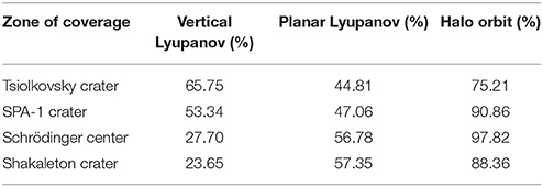
Table 1. Percentage coverage of each orbit.

It can be seen that best performing orbit is the halo orbit, and so for the purpose of providing continuous communications to a lunar ground station as well as continuous connection with stations with Earth, a halo orbit with the following initial conditions is chosen as the candidate reference orbit in this paper:

$\begin{array}{cc}\begin{array}{c}\left[\begin{array}{c}{x}_0\\ y_0\\ z_0\\ {\dot{x}}_o\\ {\dot{y}}_0\\ {ż}_0\end{array}\right]=\left[\begin{array}{c}1.12424283994529\\ 0\\ 0.187435048916681\\ 0\\ -0.223784191244108\\ 0\end{array}\right]\end{array}& (9)\end{array}$

The general problem is then to design a feedback control such that the magnitude of the error state converges to zero as t → ∞ in the presence of potentially large injection errors, SRP and only position measurements.

3. A General Active Uncertainty Measurement Control (AUMC)

The general AUMC is based on the original idea of the active disturbance rejection control (ADRC) proposed in Han [21]. ADRC is used to measure the unknown disturbances within the system and to cancel the estimated disturbance in the control at each sampling period. In this paper we refer to the coupling of a proportional controller and an ESO as AUMC as the ESO is used to measure (depending on its form) the SRP disturbance while taking into account the higher-order terms in the linearization and velocity measurement. In this section we introduce a general AUMC which combines a proportional-type controller coupled with an ESO of the form:

$\begin{array}{ll}\text{u}=-K\delta \text{x}-{\widehat{\text{x}}}_3& (10)\end{array}$

where δx = x − x_ref, K is a gain matrix that can be tuned experimentally or computed using LQR [20] by removing the unknown dynamics from the equation of motion. The current state of the spacecraft x is assumed to be measurable and ${\widehat{\text{x}}}_3$ is the output of the following ESO:

$\begin{array}{ll}\begin{array}{c}{\stackrel{·}{\widehat{\text{x}}}}_1={\widehat{\text{x}}}_2+{\beta }_1({\text{x}}_1-{\widehat{\text{x}}}_1)\hfill \\ {\stackrel{·}{\widehat{\text{x}}}}_2={\widehat{\text{x}}}_3+\text{g}(\text{x})+\text{u}+{\beta }_2({\text{x}}_1-{\widehat{\text{x}}}_1)\\ {\stackrel{·}{\widehat{\text{x}}}}_3={\beta }_3({\text{x}}_1-{\widehat{\text{x}}}_1)\hfill \end{array}& (11)\end{array}$

where ${\widehat{\text{x}}}_1$ is the estimate of x₁ (or δx₁ if the linearization of f(x₁, x₂) is used), ${\widehat{\text{x}}}_2$ is the estimate of x₂ (or δx₂ in the linear case) and ${\widehat{\text{x}}}_3$ is the estimate of

$\begin{array}{ll}h=f({\text{x}}_1,{\text{x}}_2)-g({\text{x}}_1,{\text{x}}_2)+{\text{a}}_S& (12)\end{array}$

where g(x) is a prescribed function that is defined by the control engineer depending on the control objectives, for example, it can be set to be the known nonlinear or linearized dynamics or simply set to zero. To initialize the estimator we set ${\widehat{\text{x}}}_1(0)={\text{x}}_1(0)$ and ${\widehat{\text{x}}}_2(0)={\text{x}}_2(0)$ (or ${\widehat{\text{x}}}_1(0)=\delta {\text{x}}_1(0)$ and ${\widehat{\text{x}}}_2(0)=\delta {\text{x}}_2(0)$ if the linearized dynamics are being used for control design) as these values are known and assumed to be given by the sensors, while ${\widehat{\text{x}}}_3(0)=0$ as this is an uncertain quantity. Note that this control requires the input of both the position and the velocity (or position and velocity errors in the linear case) of the spacecraft x₁, x₂ which will require both reference or optical sensors as well as an inertial measurement unit. In the case that there is a fault in the velocity measurement sensor the control law (10) can be adapted to:

$\begin{array}{ll}\text{u}=-K_1\delta {\text{x}}_1-K_2\delta {\widehat{\text{x}}}_2-{\widehat{\text{x}}}_3& (13)\end{array}$

where $\delta {\text{x}}_1={\text{x}}_1-{\text{x}}_1^{ref}$ and $\delta {\widehat{\text{x}}}_2={\widehat{\text{x}}}_2-{\widehat{\text{x}}}_2^{ref}$ where ${\widehat{\text{x}}}_2$ and ${\widehat{\text{x}}}_3$ are outputs of the ESO:

$\begin{array}{ll}\begin{array}{c}{\stackrel{·}{\widehat{\text{x}}}}_1={\widehat{\text{x}}}_2+{\beta }_1({\text{x}}_1-{\widehat{\text{x}}}_1)\hfill \\ {\stackrel{·}{\widehat{\text{x}}}}_2={\widehat{\text{x}}}_3+\text{g}({\text{x}}_1,{\widehat{\text{x}}}_2)+\text{u}+{\beta }_2({\text{x}}_1-{\widehat{\text{x}}}_1)\\ {\stackrel{·}{\widehat{\text{x}}}}_3={\beta }_3({\text{x}}_1-{\widehat{\text{x}}}_1)\hfill \end{array}& (14)\end{array}$

Defining the unknown derivative of h = x₃ as ${\stackrel{·}{\text{x}}}_3=\text{ϕ}$ and the error to be ${\text{e}}_i={\text{x}}_i-{\widehat{\text{x}}}_i$ for i = 1, 2 and ${\text{e}}_3=h-{\widehat{\text{x}}}_3$ then the error dynamics of the ESO can be defined as:

$\begin{array}{ll}\begin{array}{c}{\stackrel{·}{\text{e}}}_1={\text{e}}_2-{\beta }_1{\text{e}}_1\\ {\stackrel{·}{\text{e}}}_2={\text{e}}_3-{\beta }_2{\text{e}}_1\\ {\stackrel{·}{\text{e}}}_3=\varphi -{\beta }_3{\text{e}}_1.\end{array}& (15)\end{array}$

We adopt the general tuning method for second order active disturbance rejection controls described in Xing et al. [22] where ${\beta }_1=3{\omega }_0,{\beta }_2=3{\omega }_0^2,{\beta }_3={\omega }_0^3$ where ω₀ is denoted as the observer band-width and k is an additional tuning parameter reducing the tuning to only one parameter. Then writing e₂/ω₀ = f₂ and ${\text{e}}_3/{\omega }_0^2={\text{f}}_3$ we have

$\begin{array}{ll}\begin{array}{c}{\stackrel{·}{\text{e}}}_1={\text{f}}_2{\omega }_0-3{\omega }_0{\text{e}}_1\\ {\stackrel{·}{\text{f}}}_2={\text{f}}_3{\omega }_0-3{\omega }_0{\text{e}}_1\\ {\stackrel{·}{\text{f}}}_3=\varphi /{\omega }_0^2-{\omega }_0{\text{e}}_1.\end{array}& (16)\end{array}$

then adapting the proof in Bai et al. [23] to the higher-dimensional problem here and defining $\epsilon ={\left[{\text{e}}_1{\text{f}}_2{\text{f}}_3\right]}^T$ we write

$\begin{array}{ll}\begin{array}{c}\stackrel{·}{\epsilon }={\omega }_{0}A\epsilon +B\frac{\varphi }{{\omega }_0^2}\hfill \\ A=\left[\begin{array}{ccc}-3I_{3\times 3}& I_{3\times 3}& 0_{3\times 3}\\ -3I_{3\times 3}& 0_{3\times 3}& I_{3\times 3}\\ -I_{3\times 3}& 0_{3\times 3}& 0_{3\times 3}\end{array}\right],B=\left[\begin{array}{c}{0}_{3\times 3}\\ 0_{3\times 3}\\ I_{3\times 3}\end{array}\right]\end{array}& (17)\end{array}$

defining ${\tilde{\epsilon }}_i={\left[e_{1i}{f}_{2i}{f}_{3i}\right]}^T$ where ${\text{e}}_1={\left[e_{11}{e}_{12}{e}_{13}\right]}^T$, ${\text{f}}_2={\left[f_{21}{f}_{22}{f}_{23}\right]}^T$ and ${\text{f}}_3={\left[f_{31}{f}_{32}{f}_{33}\right]}^T$ we can re-write the expression as

$\begin{array}{ll}\begin{array}{c}\frac{d{\tilde{\epsilon }}_i}{dt}=Ã{\tilde{\epsilon }}_i+\tilde{B}\frac{{\varphi }_i}{{\omega }_0^2}\hfill \\ Ã=\left[\begin{array}{ccc}-3{\omega }_0& {\omega }_0& 0\\ -3{\omega }_0& 0& {\omega }_0\\ -{\omega }_0& 0& 0\end{array}\right],\tilde{B}=\left[\begin{array}{c}0\\ 0\\ 1\end{array}\right]\end{array}& (18)\end{array}$

which has the solution

$\begin{array}{ll}{\tilde{\epsilon }}_i(t)=exp(Ãt){\tilde{\epsilon }}_i(0)+{\displaystyle {\int }_0^t}exp\left[Ã(t-\tau )\right]\tilde{B}\frac{{\varphi }_i}{{\omega }_0^2}d\tau & (19)\end{array}$

it follows that

$\begin{array}{ll}\left|\right|{\tilde{\epsilon }}_i(t)\left|\right|\le \left|\right|exp(Ãt){\tilde{\epsilon }}_i(0)\left|\right|+\left|\right|{\displaystyle {\int }_0^t}exp\left[Ã(t-\tau )\right]\tilde{B}\frac{{\varphi }_i}{{\omega }_0^2}d\tau \left|\right|& (20)\end{array}$

where ||·|| is the Euclidean Norm then

$\begin{array}{ll}\left|\right|{\tilde{\epsilon }}_i(t)\left|\right|\le \left|\right|exp(Ãt){\tilde{\epsilon }}_i(0)\left|\right|+\frac{\left|\right|\tilde{B}{\varphi }_i\left|\right|}{{\omega }_0^2}\left|\right|{\displaystyle {\int }_0^t}exp\left[Ã(t-\tau )\right]d\tau |{|}_F& (21)\end{array}$

where ||·||_F is the Frobenius Norm of a matrix then assuming the disturbance is bounded such that ||ϕ_i|| < ∂ then

$\begin{array}{ll}\left|\right|{\tilde{\epsilon }}_i(t)\left|\right|\le \left|\right|exp(Ãt){\tilde{\epsilon }}_i(0)\left|\right|+\frac{\partial }{{\omega }_0^2}\left|\right|-{Ã}^{-1}\left[I-exp(Ãt)\right]|{|}_F& (22)\end{array}$

Then noting that the eigenvalues of à are λ = −ω₀, −ω₀, −ω₀ then exp(Ãt) → 0_{3 × 3} as t → ∞ such that in the limit

$\begin{array}{ll}\left|\right|{\tilde{\epsilon }}_i(t)\left|\right|\le \frac{\partial }{{\omega }_0^2}\left|\right|-{Ã}^{-1}|{|}_F& (23)\end{array}$

then

$\begin{array}{ll}\left|\right|{\tilde{\epsilon }}_i(t)\left|\right|\le \frac{\sqrt{21}\partial }{{\omega }_0^3}& (24)\end{array}$

This implies that ${\widehat{\text{x}}}_3\to h$ as t → ∞ to within some small bounded error which can be decreased with an increase in the gain ω₀. Furthermore, as ${\widehat{\text{x}}}_2\to {\text{x}}_2$ then $\text{g}({\text{x}}_1,{\widehat{\text{x}}}_2)\to \text{g}(\text{x})$. Therefore given the position (and velocity if it is available)as an input then the estimated output of the ESO ${\widehat{\text{x}}}_2$ converges to the velocity vector x₂ within an error bound defined by $\left|\right|{\widehat{\text{x}}}_2-{\text{x}}_2\left|\right|\le \frac{\sqrt{21}\partial }{{\omega }_0^2}$ and ${\widehat{\text{x}}}_3$ converges to the uncertain dynamics x₃ = h within an error bound defined by $\left|\right|{\widehat{\text{x}}}_3-{\text{x}}_3\left|\right|\le \frac{\sqrt{21}\partial }{{\omega }_0^2}$. Therefore, for a high-gain (ω₀ → ∞) we can assume that the error of the ESO is negligible.

3.1. Linear AUMC for Improved Convergence With Orbit Injection-Errors

Low-thrust propulsion station-keeping often linearizes the nonlinear equations about the reference trajectory, in this case a halo orbit, and applies linear control theory such as an optimal Linear control as LQR. Defining the error state δx = x − x_ref, where x(t) = [x, y, z, ẋ, ẏ, ż]^T and x_ref is the reference halo we can write (7) in the form:

$\begin{array}{ll}\frac{d(\delta \text{x})}{dt}=\text{A}(t)\delta \text{x}+\text{u}+{\text{a}}_s+\mathcal{O}(\delta {\text{x}}_2^2)& (25)\end{array}$

where where A(t) is given by

$\begin{array}{ll}\text{A}(t)=\left[\begin{array}{cc}{\text{0}}_{3X3}& {\text{I}}_{3X3}\\ {\text{U}}_{ij}& 2\text{Ω}\end{array}\right]& (26)\end{array}$

for

$\begin{array}{cc}\begin{array}{c}\Omega =\left[\begin{array}{ccc}0& 0& 1\\ -1& 0& 0\\ 0& 0& 0\end{array}\right]\end{array}& (27)\end{array}$

and U_ij is the Jacobian of U, where each term is defined as

$\begin{array}{l}{U}_{xx}=1-\frac{1-\mu }{d^3}-\frac{\mu }{r^3}+3\frac{(1-\mu ){(x+\mu )}^2}{d^5}+3\frac{\mu {(x-1+\mu )}^2}{r^5}\\ U_{yy}=1-\frac{1-\mu }{d^3}-\frac{\mu }{r^3}+3\frac{(1-\mu )y^2}{d^5}+3\frac{\mu y^2}{r^5}\\ U_{zz}=\frac{1-\mu }{d^3}-\frac{\mu }{r^3}+3\frac{(1-\mu )z^2}{d^5}+3\frac{\mu z^2}{r^5}\\ U_{xy}=3\frac{(1-\mu )(x+\mu )y}{d^5}+3\frac{\mu (x-1+\mu )y}{r^5}=U_{yx}\\ U_{xz}=3\frac{(1-\mu )(x+\mu )z}{d^5}+3\frac{\mu (x-1+\mu )z}{r^5}=U_{zx}\\ U_{yz}=3\frac{(1-\mu )yz}{d^5}+3\frac{\mu yz}{r^5}=U_{zy}& (28)\end{array}$

which can be expressed in terms of the position and velocity, writing x₁ = [δx, δy, δz], x₂ = [δẋ, δẏ, δż], where

$\begin{array}{ll}\begin{array}{c}{\stackrel{·}{\text{x}}}_1={\text{x}}_2\hfill \\ {\stackrel{·}{\text{x}}}_2=\text{C}(t)\delta \text{x}+\mathcal{O}(\delta {\text{x}}_2^2)+\text{u}+{\text{a}}_s\end{array}& (29)\end{array}$

where C(t) is the 6 × 3 matrix C(t) = [U_ij 2Ω]. Note thatusing the ESO (14) with δx from (25) as the input and setting f(x₁, x₂) = g(x₁, x₂) = C(t)δx then ${\widehat{\text{x}}}_3\to h$ as t → ∞ where $h=\mathcal{O}(\delta {\text{x}}_2^2)+{\text{a}}_s$, with the linear control taking the form

$\begin{array}{ll}\text{u}=-K\delta \text{x}-{\widehat{\text{x}}}_3& (30)\end{array}$

where ${\widehat{\text{x}}}_3$ is the output of the following Linear ESO:

$\begin{array}{l}{\stackrel{·}{\widehat{\text{x}}}}_1={\widehat{\text{x}}}_2+{\beta }_1({\text{x}}_1-{\widehat{\text{x}}}_1)\hfill \\ {\stackrel{·}{\widehat{\text{x}}}}_2={\widehat{\text{x}}}_3+\text{C}(t)\delta \text{x}+\text{u}+{\beta }_2({\text{x}}_1-{\widehat{\text{x}}}_1)\\ {\stackrel{·}{\widehat{\text{x}}}}_3={\beta }_3({\text{x}}_1-{\widehat{\text{x}}}_1)& (31)\end{array}$

as t → ∞ the closed-loop dynamics of (25) become:

$\begin{array}{ll}\begin{array}{c}{\stackrel{·}{\text{x}}}_1={\text{x}}_2\hfill \\ {\stackrel{·}{\text{x}}}_2\approx (C(t)-K)\delta \text{x}\end{array}& (32)\end{array}$

which can be expressed as $\delta \stackrel{·}{\text{x}}\approx A(K,t)\delta \text{x}$ then the gain matrix K can be chosen such that A(K, t) is point-wise negative definite and the convergence of the system has a linear response even in the presence of unknown higher-order nonlinear terms and SRP. Typically for large injection errors without an ESO a simple proportional controller would render the closed-loop dynamics nonlinear. Thus, using an ESO to compliment a linear controller can provide the guarantee of a global linear response. The performance of the linear AUMC which yields a linear response is compared to the nonlinear closed-loop response of the LQR in the following subsection.

3.1.1. Simulations

The velocity increments ΔV and the position errors of the spacecraft are important performance metrics to assess the station-keeping strategies. However, when comparing these performance metrics between LQR and AUMC there is only a small improvement when using an ESO. However, simulations show that there is an improvement in the convergence time when considering large injection-errors to within a bounded region of the reference orbit of 20 km and 0.05 m/s . In the simulations this is demonstrated for an initial injection error of δX = 100 Km, δV = 1 m/s. The observer is tuned with ω₀ = 100. In this simulation we assume the SRP is negligible. Recall that in the case of a Linear ESO the inputs are δx

Figure 1 highlights the results of halo orbits position and velocity errors encountered due to the presence of injection error of 100 Km for the LQR control. Similar results can be seen for the control AUMC in Figure 2.

FIGURE 1

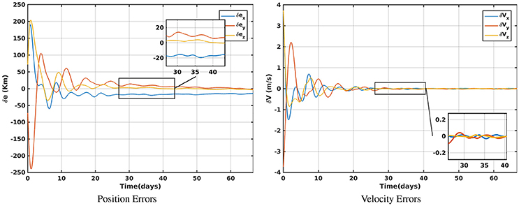
Figure 1. Errors in the position and velocity: LQR.

FIGURE 2

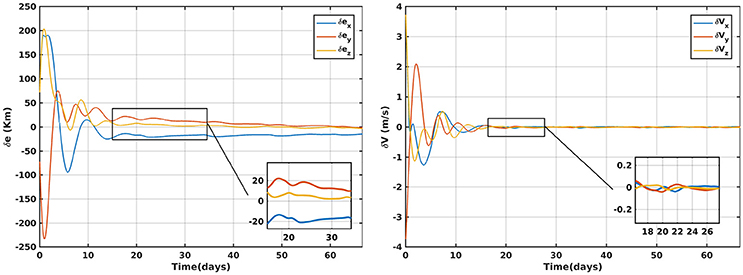
Figure 2. Errors in the position and velocity: AUMC.

It takes around 17.027 days to converge to a steady state error within 20 km compared to 27.117 days for LQR which is about of 37.2% decrease in convergence time while the error is just decreased by 4.2%.

It can be seen from Figure 3 that the control effort over time for the AUMC and the LQR is similar in magnitude and nature and therefore the ΔV is approximately the same.

FIGURE 3

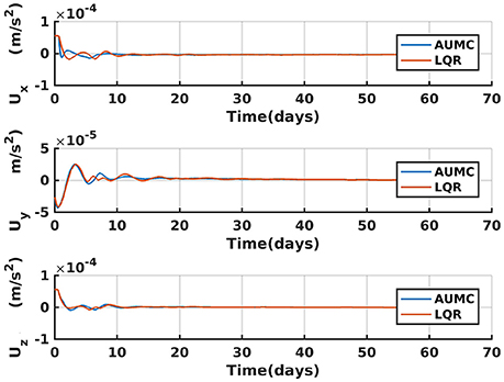
Figure 3. Control effort of LQR and AUMC.

Note that an additional possibility for the design of a linear ESO is to set g(x₁, x₂) = 0. In this case h = C(t)x+a_S and therefore as t → ∞ the output of ESO ${\widehat{\text{x}}}_3\to C(t)\text{x}+{\text{a}}_S$. Then as t → ∞ the closed-loop linear system becomes:

$\begin{array}{ll}\begin{array}{c}{\stackrel{·}{\text{x}}}_1={\text{x}}_2\hfill \\ {\stackrel{·}{\text{x}}}_2=-K\delta \text{x}\end{array}& (33)\end{array}$

Therefore, K can be chosen such that the system is asymptotically stable. In this case the closed-loop system exhibits a linear response independently. This type of control is also useful as it requires only the position of the spacecraft with respect to the reference trajectory and does not require the dynamics of the problem to be stored on-board.

3.2. Nonlinear AUMC for Velocity and SRP Estimation

In this section we consider using the control with an ESO where $g({\text{x}}_1,{\text{x}}_2)=f({\text{x}}_1,{\widehat{\text{x}}}_2)$ is described by the full-nonlinear function. In contrast to the linear ESO whose input is δx the input to the nonlinear ESO is the absolute position of the spacecraft x₁. In this case h = a_S and therefore as t → ∞ the output of ESO ${\widehat{\text{x}}}_3\to {\text{a}}_S$. Therefore, while stabilizing the spacecraft on a Halo orbit it is possible to measure the SRP a_S and given that the Sun-direction can be obtained from a Sun sensor and the position of the spacecraft is known then the uncertain coefficient a₀ can be obtained. As $\widehat{{\text{x}}_2}\to {\text{x}}_2$ as t → ∞ then $f\left({\text{x}}_1,{\widehat{\text{x}}}_2\right)\to f\left({\text{x}}_1,{\text{x}}_2\right)$. In this case as t → ∞ the closed-loop dynamics are:

$\begin{array}{ll}\begin{array}{c}{\stackrel{·}{\text{x}}}_1={\text{x}}_2\hfill \\ {\stackrel{·}{\text{x}}}_2=f({\text{x}}_1,{\text{x}}_2)-K_1\delta {\text{x}}_1-K_2\delta {\text{x}}_2\end{array}& (34)\end{array}$

although the closed-loop dynamics is independent of the SRP a linear response can only be guaranteed if f(x₁, x₂) ≈ C(t)δx. For the nonlinear stability to be guaranteed we can augment the control (35) to include a sliding-mode component and setting K₁ = kK₂ with kK₁x_i = K₂x_i = k₁x_i where k₁ is a scalar then

$\begin{array}{ll}\text{u}=-k_{1}S-{\widehat{\text{x}}}_3-k_3\text{sgn}S& (35)\end{array}$

where S defines the sliding surface S = kδx₁ + δx₂ that this is assuming that the estimator accurately measures the velocity. Then considering the Lyapunov function:

$\begin{array}{ll}V=\frac{1}{2}{S}^{T}S& (36)\end{array}$

differentiating this with respect to time and substituting in (35) yields

$\begin{array}{ll}\begin{array}{c}\stackrel{·}{V}=S^TṠ=S^T(k\delta {\stackrel{·}{\text{x}}}_1+\delta {\stackrel{·}{\text{x}}}_2)\hfill \\ =S^T(k\delta {\text{x}}_2+\text{C}(t)\delta \text{x}+\mathcal{O}(\delta {\text{x}}_2^2)-k_{1}S-k_3\text{sgn}S)\hfill \\ =-k_1{S}^{T}S-k_3{S}^T\text{sgn}S+S^T(k\delta {\text{x}}_2+\text{C}(t)\delta \text{x}+\mathcal{O}(\delta {\text{x}}_2^2))\\ \le -k_1{S}^{T}S-k_3\left|S\right|+\left|S\right||k\delta {\text{x}}_2+\text{C}(t)\delta \text{x}+\mathcal{O}(\delta {\text{x}}_2^2)|\hfill \end{array}& (37)\end{array}$

Therefore, we have asymptotic stability if $k_3>|k\delta {\text{x}}_2+\text{C}(t)\delta \text{x}+\mathcal{O}(\delta {\text{x}}_2^2)|$.

3.2.1. Simulations

In the following simulations we assume that a single side of the spacecraft and its solar panels (or a solar sail surface) is controlled to point continuously toward the Sun such that is S = n in (4). In addition for the purpose of demonstration we choose a large value for the SRP acceleration in non-dimensional units to be a₀ = 0.0798 or 0.215mms⁻² which is a typical value considered for the characteristic acceleration of the Sunjammer Solar sail [11]. However, we consider here that this value is uncertain and must be accurately estimated on-board. The nonlinear ESO is able to accurately measure the characteristic acceleration using only inputs of the position of the spacecraft. Figure 4 shows that the estimator converges to the correct value of a₀ after approximately 0.6 days. The simulation is carried out with an initial position error magnitude of 120 km. Recall that this simulation includes injection errors, large characteristic acceleration due to SRP and only position knowledge. The demonstrated simulations here only include the disturbance rejection and proportional part of the controller so that they are more readily comparable to the linear case.

FIGURE 4

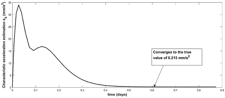
Figure 4. Plot of the output estimation of the ESO of the characteristic acceleration a₀ related to the SRP disturbance.

Figure 5 illustrates the estimated velocity in the x-direction which shows good tracking performance after an initial transient of approximately 2 days while an additional improvement in the estimation error can be seen after around 10 days.

FIGURE 5

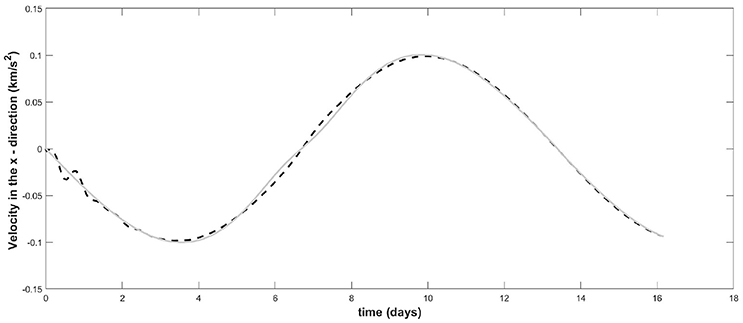
Figure 5. The ESO estimation of the velocity in the x-direction: The real velocity is in gray and the dashed line is the estimated velocity.

Figure 6 shows the tracking error over time and Figure 7 shows the corresponding control. The tracking error is within the range of 50 km although this can be improved by increasing the magnitude of the gain matrix K but at the expense of an increase in the control magnitude. The important point here is that station-keeping is achieved without knowledge of the velocity. It is not possible to obtain good tracking performance without velocity measurements or an estimate of the velocity provided by ESO.

FIGURE 6

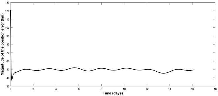
Figure 6. Tracking position error over time.

FIGURE 7

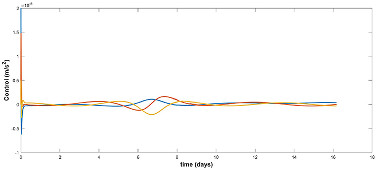
Figure 7. Control signal over time.

The simulations demonstrate that a nonlinear ESO can be useful for estimating the uncertain disturbances such as SRP in deep-space. Such information would be useful to modify the reference orbit to obtain more fuel-efficient station-keeping. Moreover, although high-fidelity solar system models are available SRP is still uncertain and an ESO provides a simple mechanism for estimating it. Furthermore, the ESO provides robustness to velocity sensor failure. In particular, without velocity information a proportional controller will perform very poorly and the tracking error can be unacceptably large. Using an ESO the tracking performance and corresponding control effort is improved significantly.

4. Conclusion

The dynamics of a spacecraft in a Lagrange point orbit are highly nonlinear and are affected by uncertain forces of solar radiation pressure. In this paper, we construct active uncertainty measurement controls for station-keeping that can guarantee asymptotic stability in the presence of orbit injection errors and SRP. The SRP acceleration parameter is estimated by the observer while station-keeping. This could be useful as accurate measures of the disturbances would allow a more accurate dynamical model of the spacecraft's orbit and the reference trajectory could be updated to a more efficient one during the mission. In addition, it is shown that station-keeping and disturbance measurements can be undertaken simultaneously using only the position knowledge of the spacecraft. This could be useful in the event that velocity sensors experience failure. This paper has demonstrated the potential uses of coupling a simple ESO with a proportional control to form an AUMC. However, there is scope for potential improvement in performance by replacing the proportional controller with other higher-performance controllers, such as sliding mode controllers, while replacing the simple ESO with nonlinear observers with the potential for greater accuracy and faster convergence. Future work could also include coupling the ESO that measures the solar radiation pressure with an on-board differential corrector so that when an accurate measure of the disturbance is obtained the reference orbit can be updated to a more natural one of the true dynamical model. In addition while we show here that the ESO can be used to measure the SRP with only knowledge of the position of the spacecraft it could be possible to use an extension of this approach to estimate highly-inhomogeneous gravity fields when orbiting asteroids or Moons. Furthermore, the mathematical demonstration of stability and the linear response of the closed-loop system in this paper relies on the assumption that the estimation error of the ESO is negligible. Future work could develop stability proofs and control laws that do not include this assumption.

Author Contributions

AN undertook extensive simulations of the comparison of LQR control and the control with an extended state observer. HH assisted in developing the mathematical proofs and writing of the paper. JB described the general extended state observer with proof of convergence and its use for improving convergence and obtaining the solar radiation pressure.

Conflict of Interest Statement

The authors declare that the research was conducted in the absence of any commercial or financial relationships that could be construed as a potential conflict of interest.

References

1. Howell KC. Three dimensional, periodic, ‘halo’orbits. Celest Mech. (1984) 32:53. doi: 10.1007/BF01358403

CrossRef Full Text | Google Scholar

2. Farquhar R. The Utilization of Halo Orbits in Advanced Lunar Operation. Greenbelt, MD: NASA TN D-6365, GSFC (1971).

Google Scholar

3. Shirobokov M, Trofimov S, Ovchinniko M. Survey of station-keeping techniques for libration point orbits. J Guid Control Dyn. (2017) 40:1085–105. doi: 10.2514/1.G001850

CrossRef Full Text | Google Scholar

4. Wie B. Space Vehicle Dynamics and Control, Chap. 2. AIAA Education Series. Reston, VA: AIAA (2008).

Google Scholar

5. Gómez G, Llibre J, Martínez R, Simó C. Dynamics and Misson Design Near Libration Points. Vol II Fundamentals: The Case of Colinear Libration Points. Singapore: World Scientific (2001).

6. Topputo F, Massari M, Biggs JD, Di Lizia P, Mani K, Dei Tos D, et al. LUMIO: Lunar Meteroid Impacts Observer. ESA contract number: 4000120225/17/NL/GLC/ac, Technical Report (2017).

7. Acton C Jr, Bachman N, Semenov B, Wright E. A look towards the future in the handling of space science mission geometry. Planet Space Sci. (2018) 150:9–12. doi: 10.1016/j.pss.2017.02.013

CrossRef Full Text | Google Scholar

8. Dachwald B, Macdonald M, McInnes CR, Mengali G, Quarta AA. Impact of optical degradation on solar sail mission performance. J Spacecraft Rock. (2007) 44:740–9. doi: 10.2514/1.21432

CrossRef Full Text | Google Scholar

9. Spencer H, Carroll KA. Real solar sails are not ideal, and yes it matters. In: Macdonald M, editor. Advances in Solar Sailing, Springer Praxis Books. Berlin; Heidelberg: Springer (2014). p. 921–40.

Google Scholar

10. McKay R, Macdonald M, Biggs J, McInnes C. Survey of highly non-keplerian orbits with low-thrust propulsion. J Guid Control Dyn. (2011) 34:645–66. doi: 10.2514/1.52133

CrossRef Full Text | Google Scholar

11. Heiligers J, Hiddink S, Noomen R, McInnes CR. Solar sail Lyapunov and halo orbits in the Earth-Moon three-body problem. Acta Astronaut. (2015) 116:25–35. doi: 10.1016/j.actaastro.2015.05.034

CrossRef Full Text | Google Scholar

12. Heiligers J, Ceriotti M, McInnes CR, Biggs JD. Design of optimal earth pole-sitter transfers using low-thrust propulsion. Acta Astronaut. (2012) 79:253–68. doi: 10.1016/j.actaastro.2012.04.025

CrossRef Full Text | Google Scholar

13. Biggs JD, McInnes CR. Solar sail formation flying for deep-space remote sensing. J Spacecraft Rock. (2009) 46:670–8. doi: 10.2514/1.42404

CrossRef Full Text | Google Scholar

14. Biggs JD, McInnes CR, Waters T. Control of solar sail periodic orbits in the elliptic three-body problem. J Guid Control Dyn. (2009) 32:318–20. doi: 10.2514/1.38362

CrossRef Full Text | Google Scholar

15. Biggs JD, McInnes CR. Passive orbit control for space-based geo-engineering. J Guid Control Dyn. (2010) 33:1017–20. doi: 10.2514/1.46054

CrossRef Full Text | Google Scholar

16. Di Giamberardino P, Monaco S. On halo orbits spacecraft stabilization. Acta Astronaut. (1996) 38:903–25. doi: 10.1016/S0094-5765(96)00082-3

CrossRef Full Text | Google Scholar

17. Cielaszyk D, Wie B. New approach to halo orbit determination and control. J Guid Control Dyn. (1996) 19:266–73. doi: 10.2514/3.21614

CrossRef Full Text | Google Scholar

18. Lian Y, Gómez G, Masdemont J, Tang G. Station-keeping of real Earth-Moon libration point orbits using discrete-time sliding mode control. Commun Nonlin Sci Numer Simulat. (2014) 19:3792–807. doi: 10.1016/j.cnsns.2014.03.026

CrossRef Full Text | Google Scholar

19. Zhu M, Karimi H, Zhang H, Gao Q, Wang Y. Active disturbance rejection station-keeping control of unstable orbits around collinear libration points. Math Prob Eng. (2014) 2014:410989. doi: 10.1155/2014/410989

CrossRef Full Text | Google Scholar

20. Narula A, Biggs JD. Fault-tolerant station-keeping on libration point orbits. J Guid Control Dyn. (2018) 41:879–87. doi: 10.2514/1.G003115

CrossRef Full Text | Google Scholar

21. Han J. From PID to active disturbance rejection control. IEEE Trans Indust Electr. (2009) 56:900–6. doi: 10.1109/TIE.2008.2011621

CrossRef Full Text | Google Scholar

22. Xing C, Donghai L, Zhiqiang G, Chuanfeng W. Tuning method for second-order active disturbance rejection control. In: Proceedings of the 30th Chinese Control Conference 22–24 July. Yantai (2011).

Google Scholar

23. Bai Y, Biggs JD, Bernelli-Zazzera F, Cui N. Adaptive attitude tracking with active uncertainty rejection. J Guid Control Dyn. (2018) 41:550–8. doi: 10.2514/1.G002391

CrossRef Full Text | Google Scholar