Nonlinear Dynamics in Coevolution of Economic and Environmental Systems

1. Introduction

The literature on economic growth has so far focused on highly stylized models¹. More recently, an increasing attention has been paid to the analysis of models which consider more realistic interplays among variables and the possible emergence of non-trivial dynamics.

In this paper, several models aimed to explore particular connections between economic activity and the environment will be examined. In particular, we will focus on the analysis of models described by dynamic systems able to highlights both the long-term trends of the variables and the emergence of short or medium-term phenomena arising from their interaction.

To this end, important models of the economic the ory, such as the Solow model, the Ramsey-Cass-Koopmans model, and the OLG structure are examined when environmental variables are introduced. In particular, we will analyse how the different approaches may affect the dynamic properties of the models. Indeed, the choice of considering the environment as productive input or as consumption good, the different hypotheses on the agents' rationality (and then the different allocative problems), and the choice between continuous and discrete time framework have relevant consequences on the models' dynamics. For example, depending on alternative assumptions, the productivity in the private sector could be effective or not in defining the complexity of the system. Moreover, another decisive axiom is related to the complementarity or substitutability between environmental and private good. Nevertheless, cyclical dynamics or multistability seem to be likely results whenever models take into account the interaction between economic and environmental systems.

The remainder of our paper is organized as follows: In section 2, we will analyse two seminal models on this issue. In section 3, we will review several models in a discrete time framework. In section 4, we will present the continuous time seminal model of Antoci et al. [2]. In section 5, we will discuss models in which a fixed time delay is introduced. Finally, section 6 will conclude.

2. Two General Frameworks

In this section, we review two milestone models in the literature on interactions between economic and environmental systems.

2.1. The Green Solow Model

One of the first models which highlights the possible existence of nonmonotonic relationships² between economic activity and the environment has been proposed by Brock and Taylor [4].³ Specifically, the authors consider an extended version of the Solow model in which savings⁴ and environmental investment choices are fixed.

In the model, the output Y is generated by a strictly concave production function F with constant returns to scale and where the inputs are the effective labor BL, where B is the labor-augmenting technological progress, and the capital K. Capital accumulates via savings, sY, with s ∈ (0, 1) and depreciates at δ > 0. The rate of labor-augmenting technological progress, g_B > 0, determines the growth rate of labor efficiency:

$\begin{array}{ll}Y=F(K,BL),\dot{K}=sY-\delta K,\dot{L}=nL,\dot{B}=g_{B}B.& (1)\end{array}$

The impact of pollution has been modeled assuming that each unit of economic activity, F, generates Ω units of pollution. Then, the amount of pollution differs from the amount generated by the economic activity only when abatement occurs. Moreover, abatement is considered as a constant returns to scale activity and the pollution abated is assumed as an increasing and strictly concave function of both the total economic activity F and the economy's ecological effort, F^A. Then, pollution is defined as:

$\begin{array}{ll}P=\Omega F-\Omega A(F,F^A)& (2)\end{array}$

where A is the abatement level. The specification can be rewritten also as:

$\begin{array}{ll}P=\Omega Fa(\theta )& (3)\end{array}$

where $a(\theta )\equiv [1-A(1,\frac{F^A}{F}\left)\right]$ and $\theta =\frac{F^A}{F}$. Combining environmental assumptions with the Solow model, the output Y becomes $\tilde{Y}=(1-\theta )F$ and, assuming also an exogenous technological process in abatement at the rate g_A > 0, it is derived:

$\begin{array}{ll}\tilde{y}=f(k)[1-\theta ]& (4)\end{array}$

$\begin{array}{ll}\dot{k}=sf(k)[1-\theta ]-[\delta +n+g_B]k& (5)\end{array}$

$\begin{array}{ll}p=f(k)\Omega a(\theta )& (6)\end{array}$

where $k=\frac{K}{BL}$, $\tilde{y}=\frac{\tilde{Y}}{BL}$, $p=\frac{P}{BL}$ and f(k) = F(k, 1).

From a dynamic point of view, the model presents a differential equation in k from which, by assuming that Inada conditions⁵ hold for F and θ fixed, the unique interior fixed point k* attracts every initial condition k(0) > 0.

Moreover, it can be noticed that, as k → k*, the aggregate output, consumption and capital approach the same growth rate g_B + n and, consequently, their per capita levels grow at the rate g_B > 0.

At the steady state level k*, the growth rate of emissions g_P is given by:

$\begin{array}{ll}{g}_P=g_B+n-g_A.& (7)\end{array}$

In order to describe the dynamic relationship between capital accumulation and emissions level, the authors introduce a definition of sustainable growth in these terms: a balanced growth path⁶ is sustainable if it is associated to both rising consumption per capita and an improving environment. In mathematical terms, it is characterized by the following conditions:

$\begin{array}{ll}{g}_B>0,g_A>g_B+n.& (8)\end{array}$

By differentiating the Equation (6) and assuming f(k) = k^α, the dynamics of the model are described by the following system:

$\begin{array}{ll}\{\begin{array}{l}\begin{array}{l}\frac{\dot{k}}{k}=s{k}^{\alpha -1}(1-\theta )-(\delta +n+g_B)\\ \frac{\dot{P}}{P}=g_B+n+\alpha \frac{\dot{k}}{k}.\end{array}\hfill \end{array}& (9)\end{array}$

Therefore, the system (9) allows to capture the evolution of emissions along time, as k → k*. By assuming sustainable growth (that is, g_P < 0), the value k_T (called turning point), ensuring $\frac{Ṗ}{P}=0$, is lower than k* and this implies that the time profile of emissions depends on the position of the initial value k₀ related to the turning point. In particular, if the economy starts with an initial capital stock such that k₀ < k_T, emissions first rise and then fall. Hence, an inverted U-shaped profile, recalling the environmental Kuznets curve, is obtained. Instead, if an initial capital stock k₀ > k_T is assumed, emissions monotonically fall as k moves toward its steady state value k*.

Finally, when the sustainable growth is not assumed, emissions grow for all t even as k approaches the steady state value.

2.2. The Ramsey-Cass-Koopmans Model With Environmental Pollution

The model in Xepapadeas [5] represents a natural evolution of the approach proposed in the previous subsection. In this context, consumption-investment choices are derived in a decentralized framework composed by intertemporal utility maximizing agents and perfectly competitive profit maximizing firms. The individual utility function depends on the per capita consumption flow c(t) and the pollution stock P(t).

The representative consumer considers the pollution level as fixed and solves the problem:

$\begin{array}{l}\underset{c(t)}{\text{max}}{\displaystyle {\int }_0^{\infty }{e}^{-\rho t}}U(c(t),P(t))dt\\ \text{subject to}{\displaystyle {\int }_0^{\infty }{e}^{-R(t)}}c(t)dt=k(0)+{\displaystyle {\int }_0^{\infty }{e}^{-R(t)}}w(t)dt\end{array}$

where ρ is the discount rate in the utility function, k(0) is the initial capital and $R(t)={\int }_{\tau =0}^{t}r(\tau )d\tau$, with r(τ) real interest rate at time τ and e^−R(t) an appropriate discount factor. Under standard assumptions of concavity on U and imposing that ${\displaystyle \underset{c\to +\infty }{lim}}{U}_c(c,P)=0$, the solution of the optimization problem, obtained with the use of the maximum principle, is interior (that is, c(t) > 0 for every t) and the consumption path is defined by:

$\begin{array}{ll}\frac{\dot{c}}{c}=\frac{1}{\eta }\left[r-\rho +\frac{U_{cP}}{U_c}\dot{P}\right]& (10)\end{array}$

where $\eta =-\frac{U_{cc}}{U_c}c$.⁷ By assuming that (i) the production function f(k) satisfies the Inada conditions, (ii) markets are competitive and firms are profit maximizers (which imply f′(k) = r + δ), the economic dynamics is described by the following system:

$\begin{array}{ll}\{\begin{array}{l}\frac{\dot{c}}{c}=\frac{1}{\eta }\left[f^{\prime }(k)-\rho -\delta +\frac{U_{cP}}{U_c}\dot{P}\right]\\ \dot{k}=f(k)-c-\delta k\\ \dot{P}=\varphi f(k)-mP.\end{array}& (11)\end{array}$

By analysing the model, a unique steady state (c*, k*, P*) exists and the dynamics, generated by an optimization process, evolve on the stable manifold of (c*, k*, P*) and converge to it. As explained in Xepapadeas [5], by considering that pollution evolves, it can be noted that the coordinates (c*, k*) are generally not affected by the stationary state value of P*, although the approach path to the steady state is affected [due to the presence of $\frac{U_{cP}}{U_c}Ṗ$ in the first equation of system (11)].

3. Discrete Time Models

If, on the one hand, the aforementioned models are suitable to describe long run trends, on the other hand they are not able to capture the occurrence of short or medium run nonlinear phenomena.

Regarding this point, the work of Day [6] provides an example of how complex phenomena may emerge from the dynamic analysis of a simple economic framework.

3.1. The Day's (1982) Model

In this work, the author considers a neoclassical growth model à la Solow (1956) in discrete time. Indeed, assuming no capital depreciation, it can be expressed by a first order difference equation in the capital-labor ratio $k_t=\frac{K_t}{L_t}$, that is

$\begin{array}{ll}{k}_{t+1}=\frac{\sigma f(k_t)}{1+\lambda }& (12)\end{array}$

where σ is the saving ratio assumed as constant, f(·) is the production function and λ is the natural growth rate of population.

By assuming that productivity is reduced by a so called pollution effect, Day [6] introduces the following specification for f:

$\begin{array}{ll}f(k)=A{k}^{\beta }{(m-k)}^{\gamma }& (13)\end{array}$

where A > 0 is a productivity parameter, β > 0 is the elasticity of capital, m > 0 is the state of environment if private production is not performed and γ > 0 weighs the effects of pollution.

Then, the map that describes the dynamics of the model becomes:

$\begin{array}{ll}{k}_{t+1}=\frac{\sigma A{k}_t^{\beta }{(m-k_t)}^{\gamma }}{1+\lambda }.& (14)\end{array}$

The map in (14) is unimodal, C¹, and admits a unique maximum point $\overline{k}=\left(\frac{\beta m}{\beta +\gamma }\right)$, from which it can be obtained the maximum capital-labor ratio $k^m=f(\overline{k})$, that is:

$\begin{array}{ll}{k}^m=\frac{A\sigma }{1+\lambda }{\beta }^{\beta }{\gamma }^{\gamma }{\left(\frac{m}{\beta +\gamma }\right)}^{\beta +\gamma }.& (15)\end{array}$

In particular, note that the slope of the production function indefinitely grows as k approaches zero and consequently, for sufficiently small initial conditions k₀ > 0, growth is positive.

For values of A sufficiently small, the stationary state is monotonically achieved either from above or below. As A increases, the steady state capital stock increases until verify the equality $k^m=\overline{k}=k^s$, where k^s is the steady state capital-labor ratio. This represents the bifurcation point from which oscillations in levels of k occur for even higher values of A.

The condition k^m ≤ m is assumed to prevent negative values of k. Then, the author derives the following sufficient condition for the existence of growth cycles, that is:

$\begin{array}{ll}\frac{\beta }{\beta +\gamma }m<\frac{A\sigma }{1+\lambda }{\beta }^{\beta }{\gamma }^{\gamma }{\left(\frac{m}{\beta +\gamma }\right)}^{\beta +\gamma }\le m.& (16)\end{array}$

Indeed, for a parameterizations satisfying such condition, the capital-labor ratio exhibits bounded oscillations (perhaps after a period of growth).

In order to determine if such cycles can be chaotic, Day [6] shows the existence of a parameter set for the map such that the theorem in Li and Yorke [7] is satisfied. For example, when β = γ = m = 1, the map (14) becomes:

$\begin{array}{ll}{k}_{t+1}=\frac{\sigma A}{1+\lambda }{k}_t(1-k_t)& (17)\end{array}$

from which, following [8], the existence of a parameter set such that:

$\begin{array}{ll}3.57\le \frac{\sigma A}{1+\lambda }\le 4& (18)\end{array}$

implies that irregular growth cycles appear (see Figure 1).

FIGURE 1

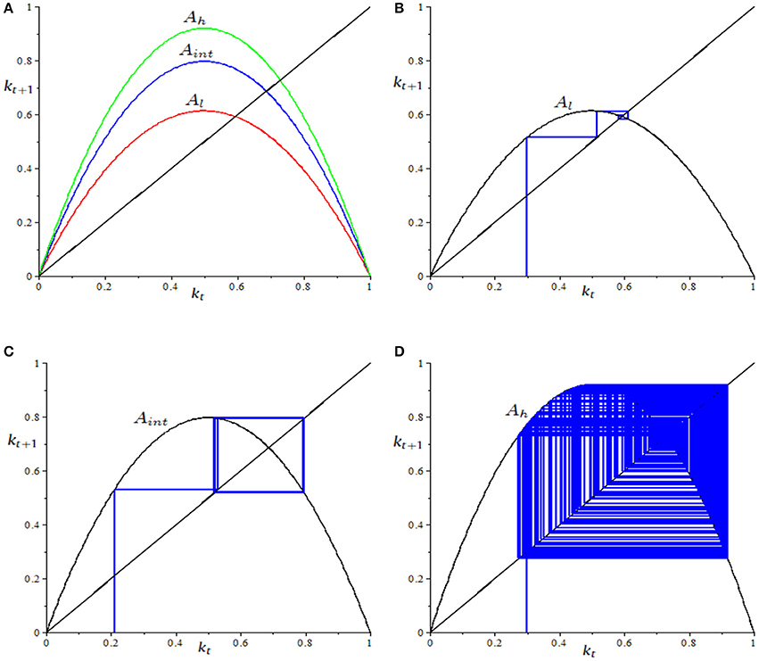
Figure 1. Parameter set: σ = 0.5, λ = 0.02, A_l = 5, A_int = 6.5, A_h = 7.5. (A) Changes in the shape of the map, as A varies. (B) Convergence to the fixed point for A = A_l (k₀ = 0.3). (C) Convergence to a 2-cycle for A = A_int (k₀ = 0.21). (D) Chaotic regime for A = A_h (k₀ = 0.3).

3.2. The Zhang's (1999) Model

In this model, the author considers an economy à la [9], in which at every period t there are two overlapping generations of individuals. The representative agent of each generation gets utility from consumption, c_t+1, and environmental quality, E_t+1, when old. The utility function U(c_t+1, E_t+1) is assumed to be increasing with respect to each argument and strictly concave. Furthermore, some Inada like conditions are satisfied, in order to get an optimal bundle with strictly positive values for c and E.

The individual supplies inelastically a unit of labor only in the first period, earning a real wage w_t, and optimally allocate w_t between private savings s_t⁸ for the old age consumption and environmental improvement expenditures, m_t. In the old age, the agent earns (1 + r_t+1 − δ)s_t, where r and δ are the real rate of return and the capital depreciation rate, respectively. Then, the individual life-cycle budget constraints are given by:

$\begin{array}{ll}{w}_t=s_t+m_t;c_{t+1}=(1+r_{t+1}-\delta )s_t.& (19)\end{array}$

The environmental quality evolves according to the following rule, staken from John and Pecchenino [9]:

$\begin{array}{ll}{E}_{t+1}=(1-b)E_t-\beta c_t+\gamma m_t& (20)\end{array}$

where b ∈ (0, 1) represents the degree of autonomous evolution of environmental quality, βc_t measures the consumption degradation of the environment, and γm_t measures the environmental improvement (β and γ are assumed to be positive). The production function f(k_t):ℝ₊ → ℝ₊ is assumed to be C² and strictly concave with respect to k_t (the capital-labor ratio). Firms maximize profits and then:

$\begin{array}{ll}{w}_t=f(k_t)-k_t{f}^{\prime }(k_t),r_t=f^{\prime }(k_t).& (21)\end{array}$

The representative agent maximizes his utility with respect to (19) and (20). Then, the first order necessary and sufficient condition for the maximization problem reads as:

$\begin{array}{ll}(1+r_{t+1}-\delta )U_c(c_{t+1},E_{t+1})-\gamma U_E(c_{t+1},E_{t+1})=0.& (22)\end{array}$

Hence, a perfect foresight competitive equilibrium is characterized by the Equation (21), the condition (22) and the market clearing condition k_t+1 = s_t.

To simplify the analysis, the author assumes a constant elasticity of substitution between consumption and environment, η_E, defined as:

$\begin{array}{ll}{\eta }_E\equiv \frac{E}{c}\frac{U_E}{U_c}>0,& (23)\end{array}$

and this allows to rewrite equation (22) as

$\begin{array}{ll}{c}_{t+1}=\frac{E_{t+1}[1+f^{\prime }(k_{t+1})-\delta ]}{{\eta }_E\gamma }.& (24)\end{array}$

From the market clearing condition, the author gets the following relationship between capital and environment:

$\begin{array}{ll}{k}_{t+1}=\frac{E_{t+1}}{{\eta }_E\gamma }& (25)\end{array}$

and then the study of the dynamics can be reduced to the analysis of the following first-order difference equation:

$\begin{array}{ll}{E}_{t+1}=\frac{{\eta }_E}{1+{\eta }_E}\left(\left[1-b-\frac{\beta (1-\delta )}{{\eta }_E\gamma }\right]E_t+[\gamma (1-\alpha (k_t))-\beta \alpha (k_t)]f(k_t)\right)& (26)\end{array}$

where $\alpha (k)\equiv \frac{k{f}^{\prime }(k)}{f(k)}$ is the capital share of output. In order to simplify the analysis, α is assumed as constant. Therefore, by considering $f(k_t)=A{k}_t^{\alpha }$ (where A > 0 represents the productivity parameter), [10] gets the expression

$\begin{array}{ll}{E}_{t+1}=a_0{E}_t+\left[\frac{A{\eta }_E^{1-\alpha }[\gamma (1-\alpha )-\beta \alpha ]}{{\gamma }^{\alpha }(1+{\eta }_E)}\right]{(E_t)}^{\alpha }\equiv G(E_t)& (27)\end{array}$

where $a_0\equiv \frac{(1-b){\eta }_E\gamma -\beta (1-\delta )}{\gamma (1+{\eta }_E)}$. It can be noticed that this parameter is less than 1 and it is independent with respect to α.

About the dynamics of the model, an interior fixed point exists if and only if γ(1 − α) − βα > 0. In particular, Zhang [10] shows that, when a₀ ≥ 0, the unique stationary equilibrium is given by

$\begin{array}{ll}{E}^{\ast }={\left[\frac{A{\eta }_E^{1-\alpha }[\gamma (1-\alpha )-\beta \alpha ]}{(1-a_0){\gamma }^{\alpha }}\right]}^{\frac{1}{1-\alpha }}& (28)\end{array}$

and the following proposition holds:

Proposition 1. Suppose γ(1 − α) − βα > 0. Then, if a₀ ≥ 0, map G is monotonically increasing; for all E₀ ∈ (0, +∞), $\underset{t\to +\infty }{lim}{G}^t(E_0)=E^{*}$. That is, there exists a unique and asymptotically stable (attracting) positive steady state.

When a₀ < 0, dynamics may exhibit complexity. By assuming $-\frac{{\alpha }^{-\frac{\alpha }{1-\alpha }}}{1-\alpha }<a_0$, [10] proves that if $a_0\in [-\frac{1+\alpha }{1-\alpha },0)$, E* is stable. Instead, if a₀ decreases in the interval $(-\frac{{\alpha }^{-\frac{\alpha }{1-\alpha }}}{1-\alpha },-\frac{1+\alpha }{1-\alpha })$, the map G exhibits the classical period-doubling sequence, summarized by the bifurcation diagram in Figure 2. It can be noticed that A does not play any role in the dynamic properties of the model: it only influences the level of E at the stationary state.

FIGURE 2

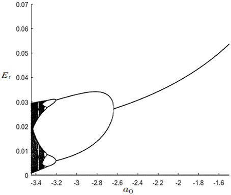
Figure 2. Occurrence of a period-doubling sequence as a₀ decreases.

3.3. The Naimzada-Sodini (2010) Model

In the case of discrete time unidimensional models with overlapping generations, a variation of the model proposed in Zhang [10], with a more general production function, has been provided by Naimzada and Sodini [11]. Remaining close to the paradigm introduced by John and Pecchenino [9], the authors propose a model in which a population of individuals is characterized by a utility function depending on the stock of an environmental good, E_t, and on the consumption of the private good, c_t. It is also assumed that E_t is negatively affected by the consumption but it is improved by specific environmental expenditures.

Differently from Zhang [10], Naimzada and Sodini [11] consider allocations in a decentralized economy. In this case, the choices of each agent between consumption and environmental expenditure generate externalities on the others. A consequence of this assumption is that the environmental maintenance, because of the environment is considered as a public good, is characterized by the classic free-riding problem. In particular, the functional form described by the authors is the following:

$\begin{array}{ll}{E}_{t+1}=(1-b)E_t-\beta {\displaystyle \sum _{i=1}^N{c}_t^i}+\gamma {\displaystyle \sum _{i=1}^N{m}_t^i}+b\overline{E}& (29)\end{array}$

where b ∈ (0, 1) measures the autonomous evolution of environmental quality, β > 0 measures the consumption effect on environment, γ > 0 weighs the environmental expenditures efficiency, N is the number of the agents, and $\overline{E}>0$ represent the long run value of the environmental index in absence of anthropic activity. Individual preferences are described by the utility function U(c_t+1, E_t+1), with U assumed as twice continuous and differentiable. Also in this case, Inada like conditions are also assumed to avoid corner solutions in the optimization problem.

On the production side, compared with [10], the model considers a more general specification, that is a CES-technology:

$\begin{array}{ll}Y=Af(k_t)=A{(\alpha k_t^{-\rho }+(1-\alpha ))}^{-\frac{1}{\rho }}& (30)\end{array}$

where k_t is the physical capital level at t, A > 0 is a scaling parameter, α ∈ (0, 1) measures the degree of capital intensity of production, and $\theta =\frac{1}{1+\rho }$ represents the elasticity of substitution between labor and capital, with ρ > 0.

From the optimality conditions, equilibrium expressions of wage rate w_t, and interest rate r_t are derived as

$\begin{array}{ll}{w}_t=A(1-\alpha ){(\alpha k_t^{-\rho }+(1-\alpha ))}^{-\frac{1+\rho }{\rho }},& (31)\end{array}$

$\begin{array}{ll}{r}_t=A\alpha k_t^{-(1+\rho )}{(\alpha k_t^{-\rho }+(1-\alpha ))}^{-\frac{1+\rho }{\rho }}.& (32)\end{array}$

By assuming that agents are identical, the problem faced by the individual born at t is:

$\underset{c_{t+1},m_{t+1}}{\text{max}}U(c_{t+1},E_{t+1}^e)$

in which

$\begin{array}{ll}{E}_{t+1}^e=(1-b)E_t-\beta N{c}_t+\gamma (m_t^i+(N-1)m_t^e)+b\overline{E}& (33)\end{array}$

represents the expected environmental quality at time t + 1 (depending on $m_t^e$, that is, the expectation of agent i about strategies of others N − 1 identical agents) and the following constraints apply:

$\begin{array}{ll}{w}_t=s_t+m_t,& (34)\end{array}$

$\begin{array}{ll}{c}_{t+1}=(1+r_{t+1}-\delta )s_t,n& (35)\end{array}$

where s_t is the saving and δ represents the depreciation rate of capital.

By assuming that the young individual at t is able to perfectly foresee the environmental index E_t+1 and recalling the Equations (31) - (32), the equilibrium conditions for all t become:

$\begin{array}{ll}-U_{c_{t+1}}(·,·)(1+r_{t+1}-\delta )+\gamma U_{E_{t+1}^e}(·,·)=0,& (36)\end{array}$

$\begin{array}{ll}{m}_t^e=m_t^{\ast },& (37)\end{array}$

$\begin{array}{ll}{E}_{t+1}=(1-b)E_t-\beta N{c}_t^{\ast }+\gamma N{m}_t^{\ast }+b\overline{E},& (38)\end{array}$

$\begin{array}{ll}{k}_{t+1}=s_t^{i\ast }.& (39)\end{array}$

In order to analyse dynamics of the model, the authors, as in Zhang [10], introduce a constant elasticity of substitution between consumption and environment, defined as:

$\begin{array}{ll}{\eta }_E\equiv \frac{E{U}_E}{c{U}_c}>0.& (40)\end{array}$

Hence, they characterize the intertemporal equilibrium conditions by means of a nonlinear difference equation in E_t:

$\begin{array}{l}{E}_{t+1}=\frac{{\eta }_E}{N+{\eta }_E}[\left((1-b)-\frac{N\beta (1-\delta )}{\gamma {\eta }_E}\right)E_t\\ +NA\left[\gamma (1-\alpha )-\beta \alpha {\left[\frac{E_t}{\gamma {\eta }_E}\right]}^{-\rho }\right]\\ \times {\left[\alpha \left(\frac{E_t}{\gamma {\eta }_E}\right)+1-\alpha \right]}^{-\frac{1+\rho }{\rho }}+b\overline{E}]\equiv Z(E_t).& (41)\end{array}$

Therefore, Naimzada and Sodini [11] describe the dynamics distinguishing between two possible cases, depending on the sign of ρ: (i) ρ < 0 and (ii) ρ > 0.

In the case (i), the authors show that the map admits a unique positive fixed point and highlights that qualitative results similar to the ones in Zhang [10] are achievable. Then, the unique fixed point E* could be attracting or repelling and, in the latter case, limit cycles or a chaotic attractor arises. However, differently from Zhang [10], the scaling parameter A affects the stability of E*. Indeed, by starting from the parameterizations $\alpha =0.831,\beta =0.55,\gamma =1.56,\delta =0.001,{\eta }_E=5,\rho =-0.4$, $A=3,b=0.52,\overline{E}=1,N=2,000$, an increase in A generates a loss of stability of E* through a period-doubling bifurcation. In addition, for A ≃ 6, the map exhibits chaotic dynamics.

In the case (ii), the map admits an odd number of fixed points and the ones with even index are unstable. Then, differently from (i), multiple equilibria may exist. In particular, the authors prove that, for ρ > > 0, three steady states exist.

An other interesting phenomenon shown by the authors is the following. By considering a parameter set for which a unique fixed point $E_1^{*}$ exists, an increase of A is able to generate, through a fold bifurcation, two new steady states $E_2^{*}$ and $E_3^{*}$, where $E_2^{*}<E_3^{*}$ is repelling and separates the basins of attraction of the two attracting fixed points $E_1^{*}$ and $E_3^{*}$. Then, a change in A may be engine of a poverty trap (see [12]).

Considering another configuration of parameters (see the parameter set in Figure 3), the authors provide another example in which a different sequence of dynamic phenomena occurs, as A varies.

FIGURE 3

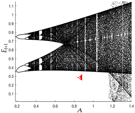
Figure 3. Parameter set: $\alpha =0.07,\beta =0.1,{\eta }_E=11,\rho =12,N=100,\delta =0.4$, $\gamma =0.04,b=0.58,\overline{E}=22$. The part of the bifurcation diagram depicted in black is generated starting from E₀ = 0.6. The part depicted in red shows the existence of a second attractor for A ∈ [0.83, 0.88] (the initial condition is E₀ = 0.29).

For A low, a unique repelling fixed point E¹, enclosed in an attracting limit 2-cycle, exists; by increasing A, the map undergoes the classic period-doubling sequence until a fold bifurcation generates two new fixed points, E² (repelling) and E³ (attracting) with E³ < E² < E¹. When A further increases, first $E_3^{*}$ loses its stability through a flip bifurcation and then a cascade of flip bifurcations appears. Moreover, there exists a region of parameters for which coexistence of attractors occurs (see Figure 3). For larger values of A, the lower attractor dies and all the feasible trajectories are attracted by the remaining attractor that lives at the right of the repelling steady state E².

Figure 4 shows an interesting global phenomenon analyzed by the authors, for even higher values of A: the remaining attractor enlarges and invades the space before occupied by the other attractor.

FIGURE 4

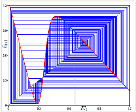
Figure 4. Merger of the attractors, A = 1.21.

Finally, an uncommon phenomenon analyzed in the work is the following one. By fixing $\alpha =0.07,\beta =0.1,{\eta }_E=11,\rho =12$, $N=100,\delta =0.4,\gamma =0.04,b=0.58,\overline{E}=22$, the second iterate of the map is characterized by two humps or more precisely by a maximum and a minimum point. By investigating the second iterate G², it can be noticed that an increase of A may lead to a fold bifurcation of G² inducing a stable 2-cycle and an unstable 2-cycle. In this case, the fold bifurcation arises far from the fixed point that maintains its instability for the whole process (see Figure 5).

FIGURE 5

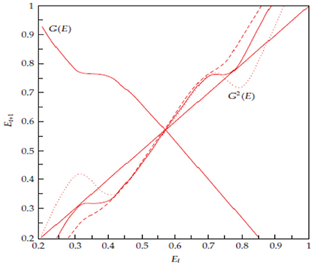
Figure 5. Figure reproduced with the permission of the authors. Source: Naimzada and Sodini [11]. Evolution of the second iterate of G (drawn at the bifurcation value A = 0.132). For A = 0.10, G² has no intersections with the main diagonal (dashed line); for A = 0.132, G² creates 2 tangent points (solid line) and for A = 0.16, two fixed points for G² are born (dotted line).

3.4. The Caravaggio-Sodini Model (2017)

Recently, by following some suggestions from empirical findings⁹, Caravaggio and Sodini [14] have proposed a model in which, by assuming an overlapping generation framework and discrete time, the environmental resource is not an argument in the agent's utility but is taken as an input in the production of a private good. Moreover, differently from John and Pecchenino [9], the model on the one hand assumes that the economic activity damages the environment and that agents consider it only as an externality¹⁰; on the other hand, it assumes that the government imposes a wage taxation with a fixed share devolved to the maintenance of a natural resource¹¹.

About the economic agent, at time t he supplies inelastically his time endowment and the earned wage w_t is allocated between the consumption c_t and the saving s_t. Hence, the individual preferences depend on consumption in the young age, c_t, consumption in the old age, d_t+1 = s_tR_t+1 and on the level of basic services provided by public sector. Thus, the utility function is given by:

$\begin{array}{ll}U(c_t,{\overline{c}}_t,d_{t+1},{\overline{d}}_{t+1},S_t)=\ln (c_t-\rho {\overline{c}}_t)+\ln (S_t)+\varphi \ln (d_{t+1}-\sigma {\overline{d}}_{t+1})& (42)\end{array}$

where ρ, σ ∈ (0, 1) represent the intensity of consumption spillover in young and old age, respectively, ϕ > 0 determines the discount factor and ${\overline{c}}_t$, ${\overline{d}}_{t+1}$ are consumption externalities. Moreover, the government levies a tax on labor wage at the tax rate τ ∈ (0, 1). Saving, remunerated at the real interest factor R_t+1, is used to consume the final good in the old age. Then, the agent has to face the following intertemporal budget constraint:

$\begin{array}{ll}(1-\tau )w_t=\frac{d_{t+1}}{R_{t+1}}+c_t.& (43)\end{array}$

Maximizing the utility function (42) with respect to (43) and considering the ex post conditions ${\overline{c}}_t=c_t$, ${\overline{d}}_{t+1}=d_{t+1}$, the saving function is obtained as:

$\begin{array}{ll}{s}_t=\frac{\varphi (1-\tau )w_t(1-\rho )}{1-\sigma +\varphi (1-\rho )}.& (44)\end{array}$

On the production side, the private good is produced through the following Cobb-Douglas technology:

$\begin{array}{ll}{Y}_t=F(k_t,{\overline{k}}_t,E_t)=A{k}_t^{\alpha }{\overline{k}}_t^{\beta }{E}_t^{\gamma },\text{with}\alpha ,\beta ,\gamma >0\text{and}\alpha +\beta \le 1& (45)\end{array}$

where ${\overline{k}}_t$ represents a production externality, A > 0 is the productivity scaling parameter and E_t is the stock of natural resource involved in the productive process. In that specification, authors assume both the possibility of decreasing social returns to scale and constant social returns to scale, that is α + β ≤ 1. From the known optimality conditions, the equilibrium expressions for wage and interest rate are derived as:

$\begin{array}{ll}{w}_t=A(1-\alpha )k_t^{\alpha }{\overline{k}}_t^{\beta }{E}_t^{\gamma }& (46)\end{array}$

$\begin{array}{ll}{R}_t=A\alpha k_t^{\alpha -1}{\overline{k}}_t^{\beta }{E}_t^{\gamma }.& (47)\end{array}$

Regarding to the evolution of natural resource, a functional form similar to the one introduced in Smulders and Gradus [16] is adopted:

$\begin{array}{ll}{E}_{t+1}=\frac{\overline{E}+G_t^{\theta }}{1+Y_t^{\lambda }},& (48)\end{array}$

where $\overline{E}>0$ represents the natural level of environmental resource, that is the level when no productive activity exists, and λ, θ > 0 weigh the environmental impact of production Y_t and the impact of public environmental expenditures G_t = δ·(τw_t).

By considering the aggregate consistency condition $k_t={\overline{k}}_t$ and the market clearing condition on the capital market k_t+1 = s_t, the dynamics of the model are driven by the following dynamic system:

$\begin{array}{ll}M:\{\begin{array}{l}{k}_{t+1}=\frac{\varphi (1-\tau )(1-\rho )(1-\alpha )A{k}_t^{\alpha +\beta }{E}_t^{\gamma }\%}{1-\sigma +\varphi (1-\rho )}\\ E_{t+1}=\frac{\overline{E}+{\left(\delta \tau (1-\alpha )A{k}_t^{\alpha +\beta }{E}_t^{\gamma }\right)}^{\theta }}{1+{(A{k}_t^{\alpha +\beta }{E}_t^{\gamma })}^{\lambda }}.\end{array}& (49)\end{array}$

Introducing the change of variables:

$\begin{array}{ll}{Y}_t=A{k}_t^{\alpha +\beta }{E}_t^{\gamma },& (50)\end{array}$

the dynamics of the model can be studied through the analysis of the following one-dimensional map:

$\begin{array}{ll}N:Y_{t+1}=A{\left(k_{t+1}\right)}^{\alpha +\beta }{\left(E_{t+1}\right)}^{\gamma }=H(Y_t)& (51)\end{array}$

where H(Y_t) is defined as:

$\begin{array}{ll}H(Y_t):=A{\left(\frac{\varphi (1-\tau )(1-\rho )(1-\alpha )Y_t}{1-\sigma +\varphi (1-\rho )}\right)}^{\alpha +\beta }{\left(\frac{\overline{E}+{\left(\delta \tau (1-\alpha )Y_t\right)}^{\theta }}{1+Y_t^{\lambda }}\right)}^{\gamma }& (52)\end{array}$

In order to analyse the dynamics of the system by studying the dynamic properties of the map N, some relationships between maps M and N are provided:

(a) 0 is a fixed point for N if and only if $(0,\overline{E})$ is a fixed point for M;

(b) Y* > 0 is a fixed point for N if and only if there exist k* and E* such that (k*, E*) is a fixed point for M;

(c) an attracting fixed point for N corresponds to an attracting fixed point for M and vice versa.

For both mathematical and economic reasons, Caravaggio and Sodini [14] distinguish the two cases (i) α + β < 1 and (ii) α + β = 1, highlighting how different parameterizations and different initial conditions may lead the economy on a bounded growth path, on an unbounded growth path or on a poverty trap path.

In particular, in the case (i), a unique interior globally stable fixed point Y* or three interior fixed points $Y_1^{*}<Y_2^{*}<Y_3^{*}$ with $Y_1^{*}$ and $Y_3^{*}$ locally stable and $Y_2^{*}$ unstable are admitted. Therefore, dynamics of N, for initial conditions on the left and the right of $Y_2^{*}$, are captured by $Y_1^{*}$ and $Y_3^{*}$ (see Figure 6A). In addition, investigating further properties of the relationship between M and N, it can be observed that starting from a positive stationary equilibrium Y* for N, an invariant set in the plane (k, E), defined by $E=(\frac{Y^{*}}{A{k}^{\alpha +\beta }}{)}^{\frac{1}{\gamma }}$, is identified. Such expression, for the parameter set considered, describes the stable manifold of the saddle point $(k_2^{*},E_2^{*})$ that separates the basins of attraction of $(k_1^{*},E_1^{*})$ and $(k_3^{*},E_3^{*})$, as depicted in Figure 6B.

FIGURE 6

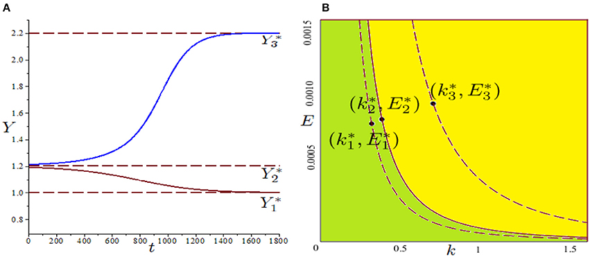
Figure 6. Figure reproduced with the permission of the publisher. Source: Caravaggio and Sodini [14]. Parameter set: $\alpha =0.32,\beta =0.6,\gamma =0.4,\delta =0.7,\theta =3,\lambda =2.87$, $\rho =0.25,\sigma =0.7,\tau =0.2,\varphi =0.6,\overline{E}=0.0007,A=48.6$. (A) Time series of Y converging to $Y_1^{*}$ or to $Y_3^{*}$ for different initial conditions; (B) Dashed lines describe iso-product curves in the plane (k, E) associated with stable fixed points of N, $Y_1^{*}$ and $Y_3^{*}$. The iso-product curve related to the unstable $Y_2^{*}$ (solid line) is the stable manifold of the saddle $(k_2^{*},E_2^{*})$ and separates the basin of attraction for $(k_1^{*},E_1^{*})$ (green region) and $(k_3^{*},E_3^{*})$ (yellow region), respectively.

Authors also highlight the particular role played by the scaling parameter A. Indeed, it can be noted that a decrease in A may cause the disappearance of the fixed points $Y_2^{*}$ and $Y_3^{*}$. Then $Y_1^{*}$ becomes the unique attractor of the system and a successive recovery of A at its original value may not allow the restoration of the previous path. Figures 7A,B provide a numerical example of this occurrence in terms of k and E.

FIGURE 7

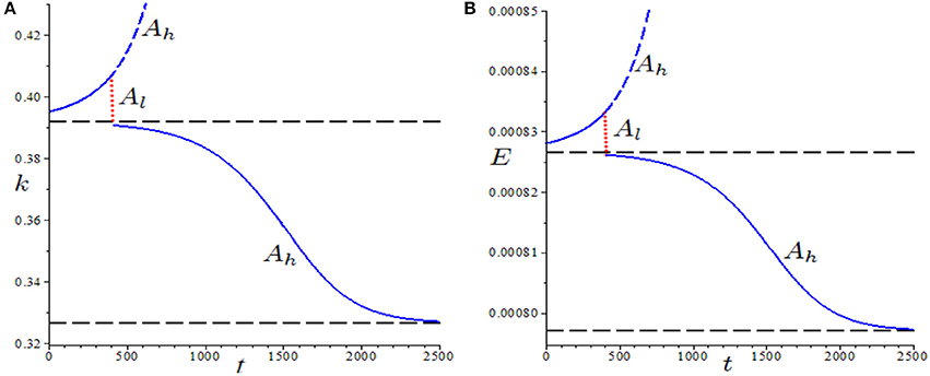
Figure 7. Figure reproduced with the permission of the publisher. Source: Caravaggio and Sodini [14]. Parameter set: $\alpha =0.32,\beta =0.6,\gamma =0.4,\delta =0.7,\theta =3,\lambda =2.87,\rho =0.25$, $\sigma =0.7,\tau =0.2,\varphi =0.6,\overline{E}=0.0007,A_h=48.6,A_l=48.3$. (A) Evolution of capital accumulation over time when a shock in A occurs; (B) Evolution of the stock of environmental resources over time when a shock in A occurs. The red pointed vertical line represents the temporary (exactly 10 iterations) time series generated by A_l.

In the case (ii), Caravaggio and Sodini [14] underline two interesting results: (1) the noninvertibility and unimodality of the map may induce the birth of nonconnected basins of attraction (see Figure 8);

FIGURE 8

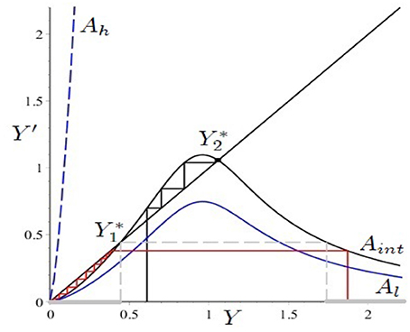
Figure 8. Figure reproduced with the permission of the publisher. Source: Caravaggio and Sodini [14]. Parameter set: $\alpha =0.6,\beta =0.4,\gamma =0.4,\delta =0.1,\theta =1.12,\lambda =8.92,\rho =0.1$, $\sigma =0.2,\tau =0.21,\varphi =0.19,\overline{E}=0.000001,A_h=5,000,A_{int}=250,A_l=150$. For A = A_int, the map admits three stationary equilibria: 0 (stable), $Y_1^{\star }=0.444$ (unstable) and $Y_2^{\star }=1.057$ (stable). The basin of 0 is nonconnected and consists of two parts: the immediate basin in $(0,Y_1^{*})$ and the other part (Y_p, +∞), where Y_p is the preimage of $Y_1^{*}$. On the contrary, the basin of $Y_2^{*}$ is connected being a single interval $(Y_1^{*},Y_p)$.

(2) For λ < θ, it is possible that trajectories, after a long transient, positively diverge. On the contrary, for λ > θ trajectories, after the transient phase, may converge to the unique attractor 0, that represents a nonproductive state for the economy (see Figures 9A,B, respectively).

FIGURE 9

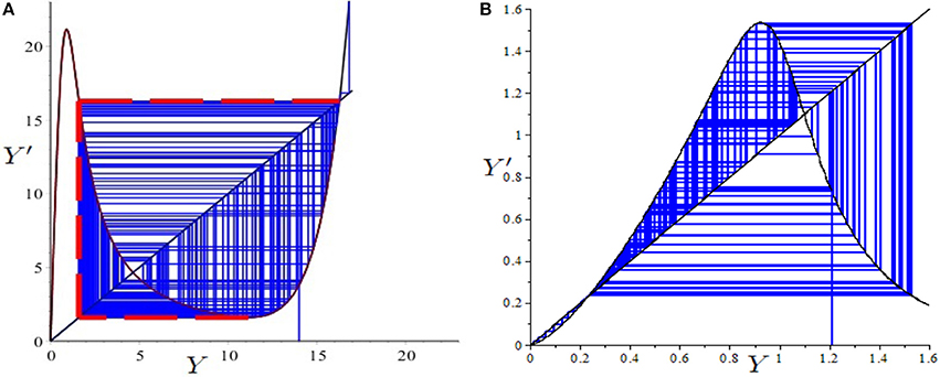
Figure 9. Figure reproduced with the permission of the publisher. Source: Caravaggio and Sodini [14]. (A) Positive divergence when λ < θ; (B) convergence to a nonproductive state when λ > θ.

3.5. The Antoci-Gori-Sodini Model (2016)

Continuing with the literature on the discrete time OLG models, several works in which a different allocation problem for the agents is taken into account have been proposed, as in Antoci and Sodini [17] and in Antoci et al. [18]. In this context, differently from John and Pecchenino [9], where the investment in environmental defensive expenditures is internalized by agents in the allocation problem, economic agents are assumed to be unable of interven for the environmental maintenance. These models therefore consider an environmental quality that is deteriorated by economic activity and individuals who defend themselves from such worsening by simply increasing the consumption of the private good, perceived as a substitute of the environmental one. As shown in Antoci and Sodini [17], since the production has a negative impact on the environment, self-protection choices induce further environmental degradation. Then, a self-enforcing mechanism may be observed according to which environmental depletion leads to an increase in the consumption of private good, which in turn generates further environmental degradation and so on.

These works show also that such self-reinforcing substitution mechanism may fuel undesirable growth paths according to which an increase in consumption of the private good is associated with a reduction in the individual well-being. Moreover, this mechanism may lead to the occurrence of several global phenomena and the individuals' expectations about the future evolution of the environmental quality can induce local and global indeterminacy.¹²

Before introducing the main features of the model in Antoci et al. [18], it can be useful to recall the definition of indeterminacy (local and global). Indeed, indeterminacy occurs if, for a given initial condition on the state variables, different values for the control variable can be chosen. In particular, if such values lead to the same Ω-limit set, then local indeterminacy occurs, otherwise if the different initial values of the control variable lead to different Ω-limit sets, then global indeterminacy arises. On the contrary, a steady state is said to be (a) locally determinate if, for an initial condition on the state variables close to the steady state, there exists, in a neighborhood of the steady state, only one feasible choice for the control variables and (b) globally determinate if, for a given initial condition on the state variables, there exists only one value of the control variables that can be chosen.

Moving on the model, the authors consider an OLG economy composed of identical and perfectly rational individuals who live for two periods, youth and old age. Each young agent allocates his time endowment between labor l_t ∈ (0, 2), remunerated at the wage rate w_t, and leisure 2−l_t. Then, the representative member of generation t earns a labor wage w_tl_t which is entirely saved at time t, that is s_t = w_tl_t. The saving s_t is invested in productive capital (K_t+1 = s_t), that the individual rents to the representative firm at the interest factor R_t+1. The revenue R_t+1s_t is used at the second period of life to buy and consume the quantity C_t+1, so that C_t+1 = R_t+1s_t. Therefore, the lifetime budget constraint of the individual of generation t is given by:

$\begin{array}{ll}{C}_{t+1}=R_{t+1}{w}_t{l}_t.& (53)\end{array}$

Individual preferences depend on leisure when individuals are young and consumption when individuals are old. In addition, the authors assume that the utility function is affected by the environmental quality, E_t+1. Then, the lifetime utility index is represented by a constant inter-temporal elasticity of substitution (CIES) function, that is:

$\begin{array}{ll}{U}_t(l_t,C_{t+1},E_{t+1})=\frac{{(2-l_t)}^{1-\gamma }}{1-\gamma }+\frac{{(C_{t+1}{E}_{t+1}^{\tau })}^{1-\sigma }}{1-\sigma }& (54)\end{array}$

where σ > 0 (σ ≠ 1) and γ > 0 (γ ≠ 1) determine the elasticity of utility with respect to consumption and leisure, respectively, and τ is a positive parameter reflecting the relative influence of environmental quality in defining the individual utility. Moreover, if σ ∈ (0, 1) (resp. σ > 1) then consumption and environment are complements (resp. substitutes). In particular, for σ ∈ (0, 1) (resp. σ > 1) the following derivative holds:

$\begin{array}{ll}\frac{{\partial }^2{U}_t(l_t,C_{t+1},E_{t+1})}{\partial C_{t+1}\partial E_{t+1}}>0(resp.<0).& (55)\end{array}$

¹³

The representative individual of generation t chooses labor supply l_t in order to maximize the value of utility function (54), subject to the intertemporal budget constraint (53) and the condition l_t ∈ (0, 2). Then, in order to get an interior solution, the necessary and sufficient first order condition for the maximization is:

$\begin{array}{ll}-{(2-l_t)}^{-\gamma }+\frac{{(R_{t+1}{w}_t{l}_t{E}_{t+1}^{\tau })}^{1-\sigma }}{l_t}=0.& (56)\end{array}$

On the production side, the authors assume that the firm produces output Y_t through a constant returns to scale Cobb-Douglas technology, that is:

$\begin{array}{ll}{Y}_t=AF(K_t,l_t)=A{K}_t^{\alpha }{l}_t^{1-\alpha }& (57)\end{array}$

where A > 0 is a scaling parameter and α ∈ (0, 1) represents the elasticity of the production function with respect to capital. By assuming that the capital stock K_t fully depreciates at the end of every period, the profit maximization implies that productive factors are remunerated at their marginal products, that is:

$\begin{array}{ll}{R}_t=\alpha A{K}_t^{\alpha -1}{l}_t^{1-\alpha },& (58)\end{array}$

$\begin{array}{ll}{w}_t=(1-\alpha )A{K}_t^{\alpha }{l}_t^{-\alpha }.& (59)\end{array}$

With regard to the environmental resource, the authors define the environmental quality index as a function that negatively depends on the economy-wide average production at time t, that is:

$\begin{array}{ll}{E}_{t+1}=\frac{\overline{E}}{1+{\overline{Y}}_t^{\rho }},& (60)\end{array}$

where $\overline{E}$ is a positive parameter symbolizing the natural value of the environmental quality, and ρ > 0 measures the environmental impact of production. It can be noticed that this specification eliminates the accumulation of environmental damages provoked by the production and, from a mathematical point of view, allows the authors to investigate the dynamical system in the plane (K_t, l_t).

By imposing the market clearing condition K_t+1 = s_t = w_tl_t, assuming that individuals have perfect foresight and that the economy-wide average output coincides, ex post, with the output of the representative firm, equilibrium conditions can be described by the following map:

$\begin{array}{ll}M:\{\begin{array}{l}\begin{array}{l}{K}_{t+1}=V(K_t,l_t)\\ =(1-\alpha )A{K}_t^{\alpha }{l}_t^{1-\alpha }\\ l_{t+1}=Z(K_t,l_t)\\ =K_t^{-\frac{{\alpha }^2}{1-\alpha }}{\left(\frac{l_t^{1-\alpha (1-\alpha )(1-\sigma )}}{{(2-l_t)}^{\gamma }}\right)}^{\frac{1}{(1-\alpha )(1-\sigma )}}{\left(\frac{{[1+{(A{K}_t^{\alpha }{l}_t^{1-\alpha })}^{\rho }]}^{\tau }}{\alpha {(1-\alpha )}^{\alpha }{A}^{1+\alpha }{\overline{E}}^{\tau }}\right)}^{\frac{1}{1-\alpha }}\end{array}\hfill \end{array}& (61)\end{array}$

where M is defined in the set $D:=\left\{(K_0,l_0)\in {ℝ}^2:K_t>0,0<l_t<2,\forall t>0\right\}$.

Regarding to existence, multiplicity and stability of fixed points, the map admits always at least one fixed point in the set D. In particular, if 0 < σ < 1, the map admits a unique fixed point, while if σ > 1, the map admits one or three fixed points, according to the natural value of the environmental quality, $\overline{E}$. Furthermore, the authors prove that for 0 < σ < 1 the fixed point is a saddle (globally determined), independently of the parameterizations; on the contrary, for σ > 1 two cases arise: (i) there exists a unique fixed point that can be a sink or a saddle independently of the parameterizations, or (ii) there exist three fixed points which have not any dynamic properties independent of the applied parameterizations. In the case (ii), given the three fixed points $(K_1^{*},l_1^{*})$, $(K_2^{*},l_2^{*})$ and $(K_3^{*},l_3^{*})$, $(K_1^{*},l_1^{*})$ and $(K_3^{*},l_3^{*})$ can be sink or saddle whereas $(K_2^{*},l_2^{*})$ can be source or saddle.

An important result shown by the authors is that, due to the absence of externalities on the production and the inclusion of the environmental variable only in the agents' utility, the map describing the dynamics of the model is invertible. This implies that, differently from Caravaggio and Sodini [14], basins of attraction are connected sets. Furthermore, the inverse map allows to numerically approximate the stable manifold of saddles, that is the trajectories converging to a determinate equilibrium.

The main issue investigated in the work is the possible rise of local and global indeterminacy. By recalling that in the model l_t is the control variable (that is, the initial value l₀ is fixed after the optimization process), while K_t is the state variable, a stationary equilibrium (K_t, l_t) is locally indetermined if it is an attractor from a dynamic point of view (in other words, it holds that for every eigenvalue λ_i, |λ_i| < 1). On the contrary, (K*, l*) is locally determined if it is a saddle, that is one of the two eigenvalues (in modulus) is larger than 1 and the other (in modulus) is smaller than one. The economic dynamics are said to be globally indetermined if there is coexistence of attractors and/or saddles.

The main configurations of the dynamics can be summarized through four examples. In the example 1, the parameter set is $A=1.25,\overline{E}=12.2,\alpha =0.2,\gamma =1.12,\sigma =3,\tau =1$. In this case, for 0 < ρ < 1 there exists a unique fixed point $(K_1^{*},l_1^{*})$ and it is a saddle (then locally determined). For ρ ≃ 1, $(K_1^{*},l_1^{*})$ becomes stable and it implies local indeterminacy. This means that, given an initial value K₀ sufficiently close to $K_1^{*}$, there exists a continuum of initial conditions l₀ such that trajectories starting from (K₀, l₀) converge to $(K_1^{*},l_1^{*})$ (see Figures 10A,B).

FIGURE 10

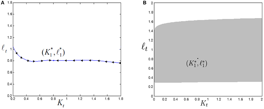
Figure 10. Figure reproduced with the permission of the publisher. Source: Antoci et al. [18]. (A) Stable manifold of the locally determined fixed point $(K_1^{*},l_1^{*})$, obtained for ρ = 0.2. (B) Basin of attraction (in gray) of the locally indeterminate fixed point $(K_1^{*},l_1^{*})$ for ρ = 1.

A further increase in ρ generates a saddle-node bifurcation from which $(K_1^{*},l_1^{*})$ and $(K_3^{*},l_3^{*})$ (attracting) and $(K_2^{*},l_2^{*})$ (saddle) are obtained. Therefore, global indeterminacy arises and then there exists initial values K₀ from which it is possible to reach all coexisting fixed points by opportunely choosing the initial value l₀, as shown in Figure 11. By further increasing the value of ρ, simultaneously $(K_1^{*},l_1^{*})$ approaches the saddle $(K_2^{*},l_2^{*})$ and $(K_3^{*},l_3^{*})$ loses its stability in favor of 2-cycle via a supercritical flip bifurcation. After the collision between $(K_1^{*},l_1^{*})$ and $(K_2^{*},l_2^{*})$ almost all trajectories belonging to D are captured by the 2-cycle arisen from $(K_3^{*},l_3^{*})$. Furthermore, the authors show that, in this case, (i) by starting from K₀ sufficiently far from $K_{3^{*}}$, there exist several l₀ such that trajectories converge to the locally determined $(K_3^{*},l_3^{*})$ and (ii) given K₀, there exist other values of l₀ for which trajectories converge to the 2-cycle. In the latter case, global indeterminacy occurs in a context in which a unique locally determined fixed point exists, as shown also in Coury and Wen [20].

FIGURE 11

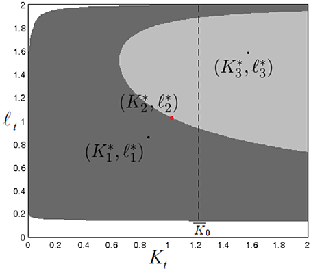
Figure 11. Figure reproduced with the permission of the publisher. Source: [18]. Global indeterminacy (ρ = 3.2): two attracting fixed points, $(K_1^{*},l_1^{*})$ and $(K_3^{*},l_3^{*})$, coexist with the saddle $(K_2^{*},l_2^{*})$.

In the example 2, considering the same parameter set of the example 1 but setting σ = 3.274, if ρ increases over the value 3.1, the system undergoes a sequence of flip bifurcations around $(K_3^{*},l_3^{*})$ (see Figure 12A). Figure 12B shows, when ρ = 3.2465, the coexistence of $(K_1^{*},l_1^{*})$ with a four-piece chaotic attractor. Because of the structure of the basins of attraction, predicting the long term behavior of the economy starting in the North-East portion of the state plane becomes rather difficult.¹⁴

FIGURE 12

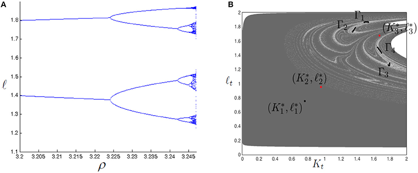
Figure 12. Figure reproduced with the permission of the publisher. Source: Antoci et al. [18]. (A) Bifurcation diagram for ρ. Due to the rise of attractors with rather tangled basins of attraction, the initial conditions were opportunely adapted to the change in ρ in order to follow the evolution of each attractor. (B) Basins of attraction when the attracting fixed point $(K_1^{*},l_1^{*})$ coexists with a four-piece chaotic attractor (ρ = 3.2465).

Finally, In examples 3 and 4, the authors show the occurrence of quasi-periodic dynamics generated via Neimark-Sacker bifurcations, further phases of coexistence and the possible rise of the phenomenon of hysteresis.

4. Continuous Time Models

The models discussed in the previous section have been sketched the main strands of literature on discrete time dynamic modeling with environment. In parallel, the literature has been enriched by several contributions developed in a continuous time framework.

For example, the existence of growth dynamics affected by the substitutability between environmental depletion and consumption of a private good, highlighted in Antoci et al. [18], have been previously analyzed in Antoci [21] in a continuous time model. In this work, the author describes growth dynamics in an economy in which the individual well-being depends on leisure, an environmental resource and a private good that can be consumed as a substitute for the environmental one. Moreover, it is assumed that the production and consumption of the substitute good impose negative externalities through the environmental deterioration. The author shows that the ratio between the technical progress and the environmental quality plays a crucial role. In particular, different dynamic systems rule the equilibrium dynamics of the model depending on such ratio and this can provoke the birth of a bistable regime. Furthermore, the work anticipates the results provided in Antoci et al. [18], in which the substitutability mechanism is engine of undesirable growth paths.

In the same way, the dynamic effects induced by the inclusion of the environmental input in the production function, analyzed in Caravaggio and Sodini [14], have been discussed through a continuous time model in Antoci et al. [2]. The results of this last contribution are described in more detail in the next subsection.

4.1. The Antoci-Russu-Galeotti Model (2011)

In this work, the authors define a growth model in which negative environmental externalities are considered and where the environment is also assumed as a productive input.

The economy is assumed to be composed by a continuum of identical agents and the representative individual produces an output Y(t) through the following Cobb-Douglas technology:

$\begin{array}{ll}Y(t)={[K(t)]}^{\alpha }{[L(t)]}^{\beta }{[E(t)]}^{\gamma },\text{with}\alpha ,\beta ,\gamma >0\text{and}\alpha +\beta <1& (62)\end{array}$

where K(t) is the stock of physical capital accumulated, L(t) is the agent's labor input and E(t) is the stock of a natural resource employed as productive input.

It is assumed an additively nonseparable utility function, as in Bennett and Farmer [22], which depends on leisure 1 − L(t) and consumption of the produced good, C(t):

$\begin{array}{ll}U[C(t),L(t)]=\frac{{[C(t){(1-L(t))}^{ϵ}]}^{1-\eta }-1}{1-\eta }& (63)\end{array}$

where η denotes the inverse of the intertemporal elasticity of substitution in consumption and ϵ, η > 0 with η ≠ 1. Moreover, the function is assumed to be concave with respect to C and 1 − L, and then the condition $\eta >\frac{ϵ}{1+ϵ}$ holds.

The evolution of K(t) is represented by the differential equation:

$\begin{array}{ll}\dot{K}=K^{\alpha }{L}^{\beta }{E}^{\gamma }-C& (64)\end{array}$

and the dynamics of the environmental resource are modeled with the well-known logistic equation augmented by the negative impact of production process:

$\begin{array}{ll}\dot{E}=E(\overline{E}-E)-\delta \overline{Y}& (65)\end{array}$

in which $\overline{E}>0$ is the carrying capacity of the natural resource, $\overline{Y}$ represents the economy-wide average output and the parameter δ > 0 measures the negative impact of production on E.

The authors assume that the representative agent chooses C(t) and L(t) in order to solve the problem

$\begin{array}{l}\underset{C,L}{\text{max}}{\displaystyle {\int }_0^{\infty }\frac{{[C{(1-L)}^{ϵ}]}^{1-\eta }-1}{1-\eta }}{e}^{-\theta t}dt\\ \text{subject to}\dot{K}=K^{\alpha }{L}^{\beta }{E}^{\gamma }-C;\dot{E}=E(\overline{E}-E)-\delta \overline{Y}\end{array}$

where K(0) and L(0) are fixed, K(t), L(t), C(t)≥0, L(t) ∈ [0, 1] and θ > 0 is the discount factor.

Since agents are identical, the ex post condition $\overline{Y}=Y$ holds. This implies that trajectories generated by the model are not socially optimal but Nash equilibria.

Starting from the Hamiltonian function associated to the optimization problem:

$\begin{array}{ll}H=\frac{{[C{(1-L)}^{ϵ}]}^{1-\eta }-1}{1-\eta }+\Omega (K^{\alpha }{L}^{\beta }{E}^{\gamma }-C)& (66)\end{array}$

in which Ω is the co-state variable associated to K, and solving the optimization problem, the authors derive the following dynamic system:

$\begin{array}{ll}\{\begin{array}{l}\dot{K}=\frac{1}{ϵ}{K}^{\alpha }{L}^{\beta -1}{E}^{\gamma }[(\beta +ϵ)L-\beta ]\hfill \\ \dot{E}=E(\overline{E}-E)-\delta K^{\alpha }{L}^{\beta }{E}^{\gamma }\hfill \\ \dot{L}=\frac{f(L)}{f^{\prime }(L)}[\frac{\alpha }{ϵ}{K}^{\alpha -1}{L}^{\beta -1}{E}^{\gamma }[(\beta +ϵ)L-\beta ]\hfill \\ +\gamma (\overline{E}-E-\delta K^{\alpha }{L}^{\beta }{E}^{\gamma -1})++\frac{1}{\eta }(\theta -\alpha K^{\alpha -1}{L}^{\beta }{E}^{\gamma })]\hfill \end{array}& (67)\end{array}$

where $f(L)=\frac{ϵ}{\beta }{(1-L)}^{\frac{ϵ-\eta (1+ϵ)}{\eta }}{L}^{1-\beta }=K^{\alpha }{E}^{\gamma }{\Omega }^{\frac{1}{\eta }}$.

Regarding to the existence of stationary states, the authors show that the system admits (i) zero, one or two stationary states if α + γ < 1, (ii) one or zero stationary states if α + γ = 1, (iii) one stationary state if α + γ > 1.

In the case (i), the authors focus on the instance in which two stationary states $P_1^{*}$ and $P_2^{*}$ exist (with $E_1^{*}<E_2^{*}$ and $K_1^{*}<K_2^{*}$). This configuration is characterized by the assumption:

$\begin{array}{ll}\overline{E}>E_A:=g(\tilde{E})=\frac{2-2\alpha -\gamma }{1-\alpha -\gamma }\tilde{E}& (68)\end{array}$

where $\tilde{E}$ is the unique positive value satisfying the condition $g^{\prime }(\tilde{E})=0$.

Analysing the Jacobian matrix J at $P_1^{*}$ and $P_2^{*}$ and using the Routh-Hurwitz criterion [23] to establish the number of eigenvalues with positive (or negative) real part, configurations of parameters for which $P_1^{*}$ is a sink, whereas $P_2^{*}$ is a saddle with a two-dimensional stable manifold are obtained.

By taking $\overline{E}$ as the bifurcation parameter, as $\overline{E}$ increases, $P_2^{*}$ does not change its nature, while $P_1^{*}$ can undergo one, two or no Hopf bifurcations.

These results show how there exist sufficient conditions to get local indeterminacy, and they are affected by the value of η,¹⁵ high enough values of δ and low enough values of θ (see the numerical example in Figure 13 where, given two initial values for the state variables (K₀, E₀) sufficiently close to their stationary values in $P_1^{*}$, there exists a continuum of initial values l₀ such that the trajectories are attracted by the limit cycle around to $P_1^{*}$).

FIGURE 13

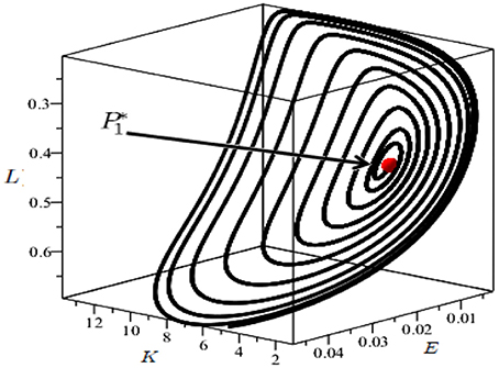
Figure 13. Parameter set: $\alpha =0.1,\beta =0.8,\gamma =0.58,\delta =0.05,ϵ=1,\eta =1.5,\theta =0.001,\overline{E}=0.21$. Locally attracting limit cycle around the unstable stationary point $P_1^{*}$ depicted in red, arisen via Hopf bifurcation.

In the case (iii), where P* is the unique stationary state, the trace of the Jacobian matrix J* is negative for some values of $\overline{E}$, and P* is a saddle with a two-dimensional stable manifold. By increasing the value of $\overline{E}$ (taken as bifurcation parameter) three chances can be obtained: (a) P* remains a saddle with a two-dimensional stable manifold and no Hopf bifurcations occur; (b) P* remains a saddle with a two-dimensional stable manifold but two Hopf bifurcations occur; (c) P* becomes a source and only one Hopf bifurcation occurs.

Regarding to the global analysis, the main result shown by the authors is the emergence of global indeterminacy. As a matter of fact, in the case (i) with $P_1^{*}$ sink and $P_2^{*}$ saddle, there exists a neighborhood N of $P_1^{*}$ such that, for every (E₀, K₀, L₀) ∈ N, the half-line {E = E₀, K = K₀, L < L₀} intersects the stable manifold of $P_2^{*}$. This means that, for every initial couple (E₀, K₀) sufficiently close to $(E_1^{*},K_1^{*})$, there exists a continuum of initial values $L_0^1$ for which the trajectory starting from $(E_0,K_0,L_0^1)$ converges to $P_1^{*}$ and a locally unique $L_0^2$ such that the trajectory starting from $(E_0,K_0,L_0^2)$ converges to $P_2^{*}$ (see Figure 14). Therefore, in this case global indeterminacy occurs.

FIGURE 14

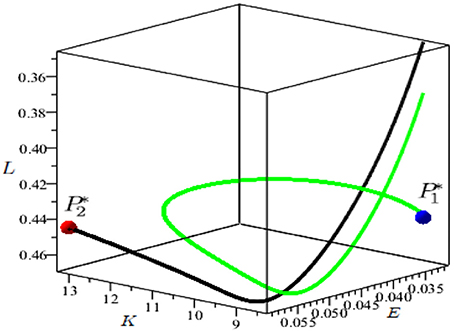
Figure 14. Parameter set: $\alpha =0.1,\beta =0.8,\gamma =0.58,\delta =0.05,ϵ=1,\eta =1.5,\theta =0.001,\overline{E}=0.17$. Global indeterminacy in the space (E, K, L). The trajectory in green approaches the sink $P_1^{*}$ (depicted in blue) starting from the point $(E_1^{*},K_1^{*},L_0^1=0.3745910588598)$, while the trajectory in black, approaching the saddle $P_2^{*}$ (depicted in red), starts from the point $(E_1^{*},K_1^{*},L_0^2=0.345910588598)$.

5. Delayed Dynamics

The interplay between economic activity and environmental quality can be finally analyzed through dynamic models where, although the time is assumed to be continuous, a time delay is introduced to underline the delayed effect of a variable on the others. Specifically, in a context in which the environmental quality is assumed, this approach turns out to be useful in showing both the noninstantaneous environmental effect of economic activity and the impact of the environmental evolution on the economy.

A seminal contribution on this issue is represented by the model described in Matsumoto and Szidarovszky [24], in which a fixed time delay is introduced in the productive sector (that is, a time to built technology is considered) and a negative environmental impact of production is assumed. The authors show that, in an extension of Day [6], chaotic dynamics may arise if a sufficiently large time delay is assumed. In particular, dynamics are described by the following equation:

$\begin{array}{ll}\dot{x}(t)=-\alpha x(t)+h(x(t-T))& (69)\end{array}$

where x is the capital per labor, α > 0 represents the depreciation ratio of capital and h defines the production function in which the fixed delay T > 0 is included.

Another significant contribution is given by Ferrara et al. [25]. In this work, the authors analyse a simplified version of the Green Solow model [4] in which the production negatively affects the environmental evolution but the environmental quality does not generate consequences on the production side. The model is defined by the following dynamic system

$\begin{array}{ll}\{\begin{array}{l}\dot{k}=s{k}_d^{\alpha }-\delta k_d\\ \dot{p}=\varphi k_d^{\alpha }-mp\end{array}& (70)\end{array}$

where k_d = k_t−τ is the individual's capital stock considering the introduction of a time lag τ > 0, p represents the stock of pollution and α ∈ (0, 1) is the capital's share. Moreover, in the first equation, s and δ > 0 denote the saving ratio and the capital depreciation rate, respectively, whereas in the second equation ϕ is the amount of emissions per unit of output and m > 0 describes the pollution decay. In the analysis, the authors provide conditions under which cyclical dynamics in the economic sector may occur and investigate how these ones may affect the environmental dynamics.

In Ferrara et al. [26], following the spirit of models provided in Wirl [27] and Antoci et al. [2], the authors consider an economy composed by agents that are not able to internalize the effect of their choices on the environmental dynamics (although they consider the environmental depletion in the utility function) but that perfectly foresee the evolution of economic variables. The novelty of the model is that the dynamics of the environmental good is assumed to be negatively affected by the economic activity that took place in an earlier date (t − τ).

More in depth, the model assumes that the representative agent produces an output Y(t) through the Cobb-Douglas technology:

$\begin{array}{ll}Y(t)=K{(t)}^{\alpha }& (71)\end{array}$

where α ∈ (0, 1) and K(t) represents the stock of physical capital employed in the production process (for simplicity, L(t) = 1 is assumed). From the environmental point of view, the following linear specification is assumed:

$\begin{array}{ll}\dot{E}=\beta (\overline{E}-E(t))-\gamma \overline{Y}(t-\tau )& (72)\end{array}$

where $\overline{Y}(t-\tau )$ is the economy-wide average output at time t − τ, $\overline{E}>0$ represents the carrying capacity of the natural resource, β > 0 measures the speed of convergence of the environmental quality toward its carrying capacity in absence of production and γ > 0 weighs the negative environmental impact of production.

The utility function U(C(t), E(t)) is dependent on the consumption of a private good and the environmental quality. Then, the following constant intertemporal elasticity of substitution (CIES) formulation is considered:

$\begin{array}{ll}U(C(t),E(t))=\frac{{[C(t)E(t)]}^{1-\sigma }}{1-\sigma }& (73)\end{array}$

where σ > 0 (σ ≠ 1) represents the inverse of intertemporal elasticity of substitution in consumption. Such specification allows to capture both cases of complementarity (σ < 1) and substitutability (σ > 1) between consumption of the private good and environmental degradation.

By assuming no depreciation of capital, the dynamics of K(t) is given by the differential equation

$\begin{array}{ll}\dot{K}=Y(t)-C(t).& (74)\end{array}$

Therefore, the representative agent faces the following intertemporal maximization problem:

$\begin{array}{l}\underset{C}{\text{max}}{\displaystyle {\int }_0^{\infty }{e}^{-rt}}\frac{{(CE)}^{1-\sigma }}{1-\sigma }dt\\ \text{subject to}\dot{K}=K^{\alpha }-C;\dot{E}=\beta (\overline{E}-E)-\gamma {\overline{Y}}_d\end{array}$

where r > 0 is the intertemporal discount rate and ${\overline{Y}}_d=\overline{Y}(t-\tau )$.

By solving the maximization problem through the use of maximum principle and imposing, ex post, the equilibrium condition ${\overline{Y}}_d^{\alpha }={\overline{Y}}^{\alpha }$, the equilibrium dynamics are described by the following system of three nonadvanced differential equations with fixed delay, that is:

$\begin{array}{ll}\{\begin{array}{l}\dot{K}=K^{\alpha }-C\\ \dot{E}=\beta (\overline{E}-E)-\gamma K_d^{\alpha }\\ \dot{C}=\frac{C}{\sigma }\{(1-\sigma )[\frac{\beta (\overline{E}-E)-\gamma K_d^{\alpha }}{E}]-(r-\alpha K^{\alpha -1})\}.\end{array}& (75)\end{array}$

On the one hand, in absence of time delays (τ = 0), the model is saddlepath stable if private consumption and the environmental good are complements and cyclical behaviors appear only assuming substitutability, in line with [18]. On the other hand, with a positive time delay, in contrast with previous results, cyclical dynamics arise also in the case of complementarity between consumption of the private good and the environmental one.

6. Conclusions

In this work we have reviewed the literature highlighting the nonlinear interactions between economic activity and environmental dynamics. We have shown that, regardless of the time setting, the dynamic systems governing the evolution of both economic and environmental variables are able to exhibit the occurrence of cyclical dynamics, multistability or indeterminacy. In addition, we have analyzed the role of some decisive parameters in defining the dynamics of the model. This set of results points out that the analysis of the global properties of dynamic systems, i.e., the structure of both basins of attraction and Ω-limit sets, represents an essential instrument to deepen these issues.

In this field, the heterogeneity in the modeling of environmental resources has not been studied yet. These heterogeneities may concern (i) the introduction of environmental variables affecting the system both as a production input and a consumption good, or (ii) the inclusion of a multiplicity of environmental resources both in the utility and production functions. The effects of this kind of heterogeneities on the dynamic properties in models focusing on the coevolution of economic and environmental variables still represent open questions on which a scholar's agenda may concentrate upon.

Finally, a fruitful research question may concern the introduction of strategic interactions between agents. In particular, it could be relevant to analyse the dynamics driven by the recognition and the achievement of environmental targets, at the international level. Indeed, as described in Biancardi and Villani [28], the decision process related international environmental agreements may generate complex relationships (multistage games) which deserves further investigations.

Author Contributions

AC, MS reviewed the literature on the coevolution of economic and environmental systems and performed the presentation (both theoretical and graphical) of all seminal contribution enclosed in the article.

Conflict of Interest Statement

The authors declare that the research was conducted in the absence of any commercial or financial relationships that could be construed as a potential conflict of interest.

Acknowledgments

The authors gratefully acknowledge Angelo Antoci, Luca Gori, Federica Nieri, and Nicla Pasquini for their valuable suggestions and comments allowing to improve the quality of the work.

Footnotes

1. ^See [1] for a survey.

2. ^See [3] for a complete review.

3. ^This work has been circulated as a working paper for many years and it was a sort of milestone for the literature of the 2000s on the relationship between growth and the environment.

4. ^This assumption is commonly used to simplify the analysis.

5. ^In economic literature, the Inada conditions are assumptions introduced in order to guarantee the stability of an interior equilibrium (see [1]).

6. ^In dynamic modeling, a balanced growth path is a trajectory such that all variables grow at constant (but potentially different) rates.

7. ^In order to simplify the notation, the subscripts denote partial derivatives. Therefore, the general equality $V_x(x,y)=\frac{\partial V(x,y)}{\partial x}=V_x$ henceforth holds.

8. ^Savings are inelastically supplied to the firms.

9. ^See for example, [13].

10. ^Agents do not invest in defensive environmental expenditures.

11. ^About the role of government in public expenditure for the environmental maintenance, see [15].

12. ^With regard to local indeterminacy in OLG models where environmental quality is considered, see also [19]. In this work, the authors show the existence of a unique stationary state and a condition for which it is locally indeterminate. In addition, differently from Zhang [10], the work underlines that the possible emergence of endogenous fluctuations does not require high levels of pollution emission rate.

13. ^The increase in U_t due to an increase in C_t+1 is positively related to the value of the index of environmental quality E_t+1 if σ ∈ (0, 1), viceversa if σ > 1.

14. ^Small changes in K₀ or l₀ may generate a change in the Ω-limit set approached by the economy.

15. ^Indeed, a further condition is given by $\eta \ge \frac{ϵ}{ϵ+\alpha \beta }$.

References

1. Barro RJ, Sala-I-Martin X. Economic Growth, 2nd Edn. Cambridge, MA: The MIT Press (2003).

2. Antoci A, Galeotti M, Russu P. Poverty trap and global indeterminacy in a growth model with open-access natural resources. J Econ Theory (2011) 146:569–91. doi: 10.1016/j.jet.2010.12.003

CrossRef Full Text | Google Scholar

3. Aghion P, Howitt P. Endogenous Growth Theory. Cambridge, MA: The MIT Press (1998).

Google Scholar

4. Brock W, Taylor MS. The green solow model. J Econ Growth (2010) 15:127–53. doi: 10.1007/s10887-010-9051-0

CrossRef Full Text | Google Scholar

5. Xepapadeas A. Economic growth and the environment. Handb Environ Econ. (2005) 3:1219–71. doi: 10.1016/S1574-0099(05)03023-8

CrossRef Full Text | Google Scholar

6. Day RH. Irregular growth cycles. Am Econ Rev. (1982) 72:406–14.

Google Scholar

7. Li TY, Yorke JA. Period three implies chaos. Am Math Monthly (1975) 82:985–92. doi: 10.1080/00029890.1975.11994008

CrossRef Full Text | Google Scholar

8. Yorke JA, Yorke E. Chaotic behavior and fluid dynamics. In: Swinney HL, Gollub JR, editors. Hydrodynamic Instabilities and the Transition to Turbulence. (Berlin: Springer) (1981). p. 77–95.

Google Scholar

9. John A, Pecchenino R. An overlapping generations model of growth and the environment. Econ. J. (1994) 104:1393–410. doi: 10.2307/2235455

CrossRef Full Text | Google Scholar

10. Zhang J. Environmental sustainability, nonlinear dynamics and chaos. Econ Theory (1999) 14:489–500. doi: 10.1007/s001990050307

CrossRef Full Text | Google Scholar

11. Naimzada A, Sodini M. Multiple attractors and nonlinear dynamics in an overlapping generations model with environment. Discr Dyn Nat Soc. (2010) 2010:503695. doi: 10.1155/2010/503695

CrossRef Full Text | Google Scholar

12. Azariadis C, Drazen A. Threshold externalities in economic development. Q J Econ. (1990) 105:501–26. doi: 10.2307/2937797

CrossRef Full Text | Google Scholar

13. Kozluk T, Zipperer V. Environmental policies and productivity growth. OECD J. (2015) 2014:155–85. doi: 10.1787/eco_studies-2014-5jz2drqml75j

CrossRef Full Text | Google Scholar

14. Caravaggio A, Sodini M. Multiple attractors and dynamics in an OLG model with productive environment. Commun Nonlinear Sci Numer Simul. (2017) 58:167–84. doi: 10.1016/j.cnsns.2017.09.019

CrossRef Full Text | Google Scholar

15. Raffin N, Seegmuller T. Longevity, pollution and growth. Math Soc Sci. (2014) 69:22–33. doi: 10.1016/j.mathsocsci.2014.01.005

CrossRef Full Text | Google Scholar

16. Smulders S, Gradus R. Pollution abatement and long-term growth. Eur J Polit Econ. (1996) 12:505–32. doi: 10.1016/S0176-2680(96)00013-4

CrossRef Full Text | Google Scholar

17. Antoci A, Sodini M. Indeterminacy, bifurcations and chaos in an overlapping generations model with negative environmental externalities. Chaos Solitons Fract. (2009) 42:1439–50. doi: 10.1016/j.chaos.2009.03.055

CrossRef Full Text | Google Scholar

18. Antoci A, Gori L, Sodini M. Nonlinear dynamics and global indeterminacy in an overlapping generations model with environmental resources. Commun Nonlinear Sci Numer Simul. (2016) 38:59–71. doi: 10.1016/j.cnsns.2016.02.005

CrossRef Full Text | Google Scholar

19. Seegmuller T, Verchère A. A note on indeterminacy in overlapping generations economies with environment and endogenous labor supply. Macroecon Dyn. (2007) 11:423–9. doi: 10.1017/S1365100506060093

CrossRef Full Text | Google Scholar

20. Coury T, Wen Y. Global indeterminacy in locally determinate real business cycle models. Int J Econ Theory (2009) 5:49–60. doi: 10.1111/j.1742-7363.2008.00102.x

CrossRef Full Text | Google Scholar

21. Antoci A. Environmental degradation as engine of undesirable economic growth via self-protection consumption choices. Ecol Econ. (2009) 68:1385–97. doi: 10.1016/j.ecolecon.2008.09.009

CrossRef Full Text | Google Scholar

22. Bennett RL, Farmer RE. Indeterminacy with non-separable utility. J Econ Theory (2000) 93:118–43. doi: 10.1006/jeth.1999.2633

CrossRef Full Text | Google Scholar

23. Hurwitz A. On the conditions under which an equation has only roots with negative real parts. Math Ann. (1895) 46:273–84.

24. Matsumoto A, Szidarovszky F. Asymptotic behavior of a delay differential neoclassical growth model. Sustainability (2013) 5:440–55. doi: 10.3390/su5020440

CrossRef Full Text | Google Scholar

25. Ferrara M, Guerrini L, Sodini M. Stability and nonlinear dynamics in a Solow model with pollution. Nonlinear Anal Model Control (2014) 19:565–77. doi: 10.15388/NA.2014.4.3

CrossRef Full Text | Google Scholar

26. Ferrara M, Gori L, Sodini M. A continuous time economic growth model with time delays in environmental degradation. J Inform Optim Sci. (2018).

27. Wirl F. Stability and limit cycles in one-dimensional dynamic optimisations of competitive agents with a market externality. J Evol Econ. (1997) 7:73–89. doi: 10.1007/s001910050035

CrossRef Full Text | Google Scholar

28. Biancardi M, Villani G. International environmental agreements with developed and developing countries in a dynamic approach. Nat Resour Model. (2014) 27:338–59. doi: 10.1111/nrm.12037

CrossRef Full Text | Google Scholar