Spectral Functional-Digraph Theory, Stability, and Entropy for Gene Regulatory Networks

1. Introduction–Spectral Theory of Functional Digraphs

1.1. Digraphs, Relations, and Functions

We will refer to a finite graph with directed edges, possibly including directed loops and directed 2-cycles, but no parallel edges, as a digraph. A vertex-labeled digraph represents a relation R on the set of labels, where a directed edge a → b indicates that aRb: hence, the common convention to include loops and opposite directed edges in the definition. When a labeled digraph has exactly one outgoing edge per vertex, it represents an ordinary function F; an edge a→b now tells us that F(a) = b. These are the functional digraphs, also known as maximal directed pseudoforests or directed 1-forests.

On the left-hand side of Figure 1, we have the digraph of a transitive relation on the set {a, b, c, d, e, f}. The digraph on the right depicts an endofunction on the same set, where the images must eventually get trapped in a directed cycle. Endofunctions on a set of n elements are in 1-1 correspondence with the digraphs on n vertices, labeled by this set, where every component contains exactly one directed cycle, and every vertex on such a cycle is the root of a directed in-tree. This is precisely why permutations of a finite set have unique cycle representations. The leaves of the in-trees correspond to the elements of the set that have no pre-images, which are among the transient (non-cycle) vertices.

FIGURE 1

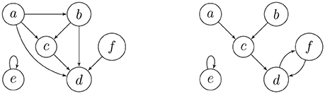
Figure 1. Digraphs for a transitive relation and a function.

1.2. Adjacency Matrices

Let S = {s₁, …, s_N} be a finite set, and R ⊆ S × S be a relation on S. The adjacency matrix, A(G), of a digraph G labeled by S is the N × N matrix given by A(G)_ij = 1 if there exists a directed edge or loop from s_i to s_j, and 0 otherwise. Although the matrix depends on the particular ordering of the vertices, its spectral properties remain unchanged under a simultaneous permutation of the rows and columns; hence, we may call such a matrix the adjacency matrix of the unlabeled digraph. The permutation can be obtained by conjugating A(G) by a permutation matrix. Two labeled digraphs are isomorphic if and only if their adjacency matrices are similar via a permutation matrix. A diagonal entry A(G)_ii is nonzero (i.e., equal to 1) if and only if there is a loop at the vertex s_i. This fact can be generalized to the following well-known statement ([1]) by induction:

Lemma 1. Let G be a digraph and A be its adjacency matrix. Then the number of directed walks from vertex s_i to vertex s_j of length k is given by the entry ${(A^k)}_{ij}$ of the matrix power A^k.

Remark 1. Let A be the adjacency matrix of a relation R. Then

1. R is reflexive if and only if every diagonal entry of A is 1.

2. R is symmetric if and only if A is a symmetric matrix.

3. R is transitive if and only if whenever ${(A^2)}_{ij}>0$, we have A_ij = 1 ¹.

Example 1. The adjacency matrices of the digraphs in Figure 1 are

$A=\left(\begin{array}{llllll}0\hfill & 1\hfill & 1\hfill & 1\hfill & 0\hfill & 0\hfill \\ 0\hfill & 0\hfill & 1\hfill & 1\hfill & 0\hfill & 0\hfill \\ 0\hfill & 0\hfill & 0\hfill & 1\hfill & 0\hfill & 0\hfill \\ 0\hfill & 0\hfill & 0\hfill & 0\hfill & 0\hfill & 0\hfill \\ 0\hfill & 0\hfill & 0\hfill & 0\hfill & 1\hfill & 0\hfill \\ 0\hfill & 0\hfill & 0\hfill & 1\hfill & 0\hfill & 0\hfill \end{array}\right)\text{ and }B=\left(\begin{array}{llllll}0\hfill & 0\hfill & 1\hfill & 0\hfill & 0\hfill & 0\hfill \\ 0\hfill & 0\hfill & 1\hfill & 0\hfill & 0\hfill & 0\hfill \\ 0\hfill & 0\hfill & 0\hfill & 1\hfill & 0\hfill & 0\hfill \\ 0\hfill & 0\hfill & 0\hfill & 0\hfill & 0\hfill & 1\hfill \\ 0\hfill & 0\hfill & 0\hfill & 0\hfill & 1\hfill & 0\hfill \\ 0\hfill & 0\hfill & 0\hfill & 1\hfill & 0\hfill & 0\hfill \end{array}\right)$

respectively (left to right). We observe that

$A^2=\left(\begin{array}{llllll}0\hfill & 0\hfill & 1\hfill & 2\hfill & 0\hfill & 0\hfill \\ 0\hfill & 0\hfill & 0\hfill & 1\hfill & 0\hfill & 0\hfill \\ 0\hfill & 0\hfill & 0\hfill & 0\hfill & 0\hfill & 0\hfill \\ 0\hfill & 0\hfill & 0\hfill & 0\hfill & 0\hfill & 0\hfill \\ 0\hfill & 0\hfill & 0\hfill & 0\hfill & 1\hfill & 0\hfill \\ 0\hfill & 0\hfill & 0\hfill & 0\hfill & 0\hfill & 0\hfill \end{array}\right)\text{and }{B}^2=B^4.$

Comparing A to A² helps us affirm transitivity, and we will see the significance of the equality of two powers of B in Theorems 1 and 2 below.

Some notation: Let 1 denote any column vector with entries of 1 only. Also, if C is a subset of the N vertices of a functional digraph, then let 1_C be the N × 1 indicator vector with entries of 1 corresponding to elements of C and 0's elsewhere. We will moreover denote by X^T the transpose of any matrix or vector X, and by e_i the ith standard basis vector of ℝ^N. We recall that Ae_j is the jth column and $e_i^{T}A$ is the ith row of A.

Lemma 2. Let A be the adjacency matrix of a digraph on the vertex set S = {s₁, …, s_N}. Then $1^{T}A{e}_j$ is the in-degree of vertex s_j, and $e_i^{T}A1$ is the out-degree of vertex s_i. If C ⊆ S, then $1_C^{T}A{e}_j$ is the number of incoming edges to vertex s_j from the vertices in C, and $e_i^{T}A{1}_C$ is the number of outgoing edges from vertex s_i to the vertices in C.

1.3. Eigenvalues and Eigenvectors of Functional Digraphs

Every row of the adjacency matrix A of a functional digraph contains exactly one entry of 1, and columns corresponding to leaves contain only 0's. Moreover, the number of directed walks of every length k ≥ 1 between two given vertices is always 0 or 1, and we reach a unique vertex after following a directed k-path from any given vertex. Hence, as we continue to take powers of A, every row will still contain a unique entry of 1, so that at some kth iteration one of the previous powers of A will be repeated, or else the matrix A^k will become the identity.

Theorem 1. Let G be a functional digraph on the vertex set S = {s₁, …, s_N}, corresponding to a function F : S → S, and A be its N × N adjacency matrix. Then the following hold:

1. The minimal polynomial of A divides a polynomial of the form x^k − x^s = x^s(x^{k − s} − 1), where N ≥ k > s ≥ 0.

2. The real eigenvalues of A are 1 and possibly 0 and/or −1.

3. The N × 1 vector 1 is always a 1-eigenvector of A.

4. Zero is an eigenvalue of A if and only if G is not entirely made up of disjoint cycles. The nullity of A is the number of its zero columns as well as the number of leaves in G.

Proof. 1. We have argued that A^k = A^s for some k > s ≥ 0.

2. The minimal and characteristic polynomials of A have the same roots with possibly different algebraic multiplicities.

3. Because there is exactly one 1 in each row of A, we have A1 = 1.

4. Apply Gaussian elimination to the matrix 0·I − A = −A. Rows with −1's that are all in one particular column are identical and can be reduced to one nonzero row, thus, the number of columns of −A that contain any −1's is the rank of the matrix. Therefore, the nullity of A is exactly the number of zero columns. These are indexed by the leaves. If G consists of cycles only, then 0 is not an eigenvalue, and A is invertible.□

With a suitable ordering of the vertices, we can write the adjacency matrix of a functional digraph in upper-triangular block form, where each triangular block on the diagonal corresponds to a connected component.

Example 2. Consider the functional digraph in Figure 1, whose adjacency matrix B with respect to the alphabetical ordering of the vertices is given in Example 1. However, when we regroup the vertices into connected components and write transient vertices before the cyclic ones, an upper-triangular block form emerges: for the ordering e, a, b, c, d, and f, the adjacency matrix becomes

The second component is represented by a 5 × 5 matrix with a 3 × 3 upper-left block for the transient vertices and a 2 × 2 lower-right block for the cycle vertices, where the latter is a circulant submatrix. The characteristic polynomial of the first component is x − 1, and that of the second component is x³ times x² − 1. In particular, since there are no directed 3-walks in the transient subgraph, the cube of the 3 × 3 block must be the zero matrix.

Theorem 2. Let G be a functional digraph with ν connected components, where the ith component has a directed c_i-cycle and t_i transient vertices. Also, let A be the adjacency matrix of this digraph. Then

1. The characteristic polynomial of A is given by ${\displaystyle \prod _{i=1}^v{x}^{t_i}}\left(x^{c_i}-1\right)$.

2. The algebraic multiplicity of 0 is the total number of transient vertices in G, whereas the geometric multiplicity is the total number of the leaves (and the number of the zero columns) of A. If A is not invertible, then the 0-eigenspace has a basis consisting of one standard basis vector e_i = 1_si for each leaf s_i.

3. The algebraic and geometric multiplicities of the eigenvalue 1 are both equal to ν, the number of cycles and connected components. A basis for the 1-eigenspace is given by

$\left\{{\mathbf{1}}_C:Cisa\underset{\_}{connectedcomponent}ofG\right\}.$

4. The algebraic and geometric multiplicities of the eigenvalue −1 (if any) is the number of even cycles in G.

Proof: Part 1 follows from multiplicativity. The explanation of Part 2 is in Example 2 and Theorem 1. For Part 3, we check that the linearly independent indicator vectors 1_C are indeed 1-eigenvectors of A: we have A1_C = 1_C if and only if $e_i^{T}A{1}_C=e_i^T{1}_C$ for all i. The left-hand side in the last identity is the number of outgoing vertices from s_i into C by Lemma 2, and must be 1 if F(s_i) ∈ C (hence, s_i ∈ C) and 0 otherwise. Since the right-hand side is the ith entry of 1_C, we are done. Finally, note that −1 is a root of $x^{c_i}-1$ if and only if c_i is even.□

1.4. The Transition Matrix

We will call the transpose A^T of the adjacency matrix A of a functional digraph the transition matrix of the corresponding function F on the vertices: A^T is clearly the matrix of the linear transformation F:ℝ^N → ℝ^N, where the vertices of the digraph form an ordered basis of ℝ^N, and F is uniquely defined by its values on the basis elements.

Theorem 3. Let A be the adjacency matrix of a functional digraph on S = {s₁, …, s_N}. Then the following hold:

1. A basis for the 1-eigenspace of A^T is given by the indicator vectors 1_C for each directed cycle C of the digraph.

2. Zero is an eigenvalue if and only if the digraph has transient vertices. When this is the case, a basis for the 0-eigenspace is found as follows: Let s_k be any vertex with in-degree at least two, say,

$F^{-1}(\{s_k\})=\{s_{i_1},\dots ,s_{i_t}\},t\ge 2,i_1<\cdots <i_t.$

3. Then the following are linearly independent 0-eigenvectors of A^T:

$e_{i_1}-e_{i_2},e_{i_1}-e_{i_3},\dots ,e_{i_1}-e_{i_t}.$

The union of these sets of vectors over all s_k with in-degree ≥ 2 is a basis for the 0-eigenspace.

Proof: 1. If we show that $A^T{1}_C=1_C$ for each cycle C, then we will have sufficiently many linearly independent indicator vectors to make up a basis. This is the same as verifying that $1_C^{T}A=1_C^T$, or, that $1_C^{T}A{e}_j=1_C^T{e}_j$ for all j. The left-hand side is the number of incoming edges to vertex s_j from the cycle C by Lemma 2. Cycle vertices cannot map to transient ones in a functional digraph, so we must have $1_C^{T}A{e}_j=1$ if s_j ∈ C and 0 otherwise. This property also describes the entries of the indicator vector $1_C^T$.

2. Let us solve A^TX = 0 for X = ∑x_ie_i. We have

$A^T\left({\displaystyle \sum _{i=1}^N{x}_i}{e}_i\right)={\displaystyle \sum _{i=1}^N{x}_i}{A}^T{1}_{s_i}={\displaystyle \sum _{i=1}^N{x}_i}{1}_{F(s_i)}=0,$

since A^T is the transition matrix that sends e_i = 1_si to 1_F(si), which is some standard basis vector e_k = 1_sk. We rewrite this linear equation by combining the coefficients of distinct vectors 1_F(si) and utilize linear independence. If s_i is the only vertex that goes to F(s_i), then the vector 1_F(si) has coefficient x_i, which must be zero in all solutions X. The only free variables will come from the coefficients of those 1_F(si) = 1_sk for which $\left|F^{-1}(s_k)\right|\ge 2$. Fix one vertex s_k, and say $F^{-1}(\left\{s_k\right\})=\left\{s_{i_1},\dots ,s_{i_t}\right\}$, with t ≥ 2 and i₁ < ⋯ < i_t. Then we can write this sub-system as x_i1 = − x_i2 − x_i3 − ⋯ − x_it, where all x_j not appearing in the equation must take the value 0. Hence, x_i2, x_i3, …, x_it are free variables, and a basis for the solutions of this system is given by

$e_{i_1}-e_{i_2},e_{i_1}-e_{i_3},\dots ,e_{i_1}-e_{i_t}.$

□

1.5. An Algorithm for Identifying Cycles and In-Trees

Let A be the adjacency matrix of a functional digraph, G, where the corresponding function F is defined on vertices s₁, …, s_N. In sections 1.3 and 1.4, we found that the task of breaking up G into its components, cycles, and in-trees can be carried out by finding suitable bases for the 0- and 1-eigenspaces of A and A^T –any software will likely produce eigenvectors in the desired form– and putting the results together. Our final algorithm ([2]) uses a hybrid method for computing cycles and their in-trees as data structures. Given a function F and its adjacency matrix, we apply Algorithm 1 above, where the array value AR[v] is the pre-image set F⁻¹(v) for any vertex v, and T_r is one of the in-trees rooted on a cycle C_k. This method is more general than one given in 1994 by Wuensche [3] (in that it does not depend on where the function comes from, namely, a GRN) and uses the eigenspace computations described in Theorem 3. The “children” of a vertex are those that are at the beginning of incoming edges.

ALGORITHM 1

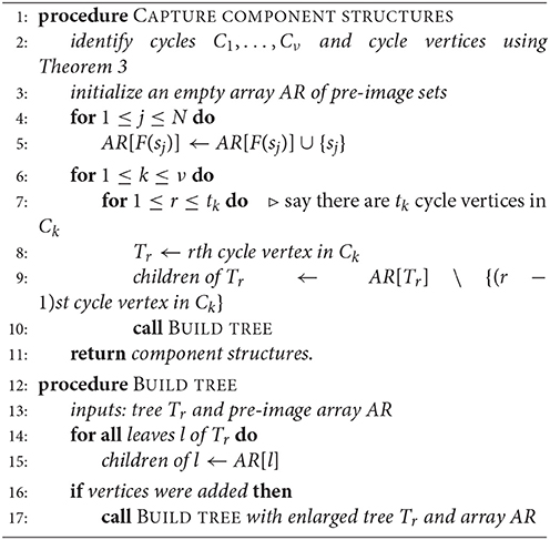
Algorithm 1 Identify cycles and in-trees for function F

1.6. The Trace

Here is yet another way to determine the number and lengths of cycles in a functional digraph G with adjacency matrix A, using Lemma 1 and simple matrix operations, with no need for eigenvector calculations. The number of 1-cycles in G is tr(A). Suppose that s_i and s_j form a 2-cycle. Then the number of directed 2-walks from s_i (resp., s_j) to itself is 1. We may also embark on a directed 2-walk from a fixed point of the function to itself by going around its loop twice, which is possible because 1 divides 2. Otherwise, if a vertex is transient, or on a larger cycle, then advancing two vertices under the function will never get us back to the same vertex. Therefore, the number of 2-cycles in G is [tr(A²) − tr(A)]/2, division by two assuring us that we are counting 2-cycles and not vertices in 2-cycles. Let us generalize, using the notation i|k to mean “i divides k.”

Theorem 4. Let G be a functional digraph on N vertices and A be its adjacency matrix. The number n_k of k-cycles in G is given recursively by

$n_1=\text{tr}(A),and{n}_k=\frac{1}{k}\left[\text{tr}(A^k)-{\displaystyle \sum _{i|k,i<k}i}{n}_i\right]for1<k\le N.$

Consequently, the number of connected components of G is equal to

$\nu ={\displaystyle \sum _{k=1}^N{n}_k}.$

2. Automorphisms and Entropy of Functional Digraphs

2.1. Digraph Automorphisms

The automorphism group Aut(G) of a labeled digraph G is the set of permutations of its vertices that preserve directed edges, and is naturally a subgroup of the full symmetric group on all vertices of G under composition. Let S_n denote the symmetric group on n letters and Hⁿ denote the direct product of n copies of a group H. Recall that the wreath product H ≀ S_n of H by S_n is a semidirect product of Hⁿ by S_n, where S_n acts on Hⁿ via permutations of the factors (4). The following is an adaptation of the well-known result for undirected graphs ([5]).

Theorem 5. Suppose that a labeled digraph G consists of n_j copies of a connected component G_j for 1 ≤ j ≤ ν, where the G_j are mutually non-isomorphic. Then the automorphism group of G is isomorphic to the following Cartesian product:

$Aut(G)\simeq [Aut(G_1)\wr S_{n_1}]\times \cdots \times [Aut(G_{\nu })\wr S_{n_{\nu }}].$

Hence, the order of Aut(G) is

$|Aut(G)|={\displaystyle \prod _{j=1}^{\nu }|}Aut(G_j){|}^{n_j}{n}_j!.$

Lemma 3. Let Aut(G) denote the automorphism group of a digraph G whose vertices are labeled by a set S = {s₁, …, s_N}. Then the number of distinct relations on S that are represented by the unlabeled digraph is equal to the index of Aut(G) in the full permutation group S_N of S, namely,

$[S_N:Aut(G)]=\frac{N!}{|Aut(G)|}.$

2.2. Identifying Similar Structures in Functional Digraphs

To define automorphism groups correctly, we need to determine whether two in-trees, or two connected components, are isomorphic.

2.2.1. In-Trees

Read [6] describes a 1-1 correspondence of rooted trees with a canonical list of binary codes. Two rooted trees are isomorphic if and only if they have the same code. We imagine the root of a given rooted in-tree placed at the top of a diagram. A vertex that is immediately below another one is referred to as the “child” of the latter, whereas the upper one is the “parent.” Hence, the arrows point upward, as this is the actual structure of the digraph. An algorithm for assigning a code (Algorithm 2) and an example (Figure 2) are given below.

ALGORITHM 2

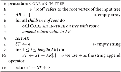
Algorithm 2 Code a rooted tree

FIGURE 2

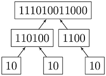
Figure 2. How to code a rooted tree.

2.2.2. Cyclic Lists

Let ℓ = ABC…  be a finite ordered list of r symbols, with r ≥ 1. The cyclic group ℤ_r acts transitively on the set ${M}$ of all cyclic permutations of ℓ, with the generator advancing each symbol one place forward, and moving the last one to the front. There is a unique stabilizer of any list in ${M}$, isomorphic to ℤ_s for some s such that s|r. Now, every cyclic list of order r has a prime (smallest) repeating block of length k; for the cyclic list ABCD, it is the whole list, and for ABABABAB, it is AB (and not ABAB, etc.) Then s = r/k, the number of blocks of ℓ.

A simple way to check whether two lists of length r are cyclically equivalent is to double one and search for the other as a string inside. For large lists, we use a modified Knuth-Morris-Pratt (KMP) string-searching algorithm [7] to find the length of each prime block [2]. A faster alternative would be the algorithm described in a paper by Shiolach [8], but it is more complex and error-prone to implement. Once a prime block is identified, we apply the so-called Lyndon factorization [9] to find the lexicographically minimal version [2]. Then two cyclic lists of the same length are equivalent if and only if their lexicographically minimal rotations are equal. A connected component of a functional digraph is a cyclic list where equal symbols denote isomorphic in-trees, and the trees are cyclically ordered by their roots on the directed cycle.

2.3. Algorithm for the Automorphism Group of a Functional Digraph

2.3.1. Automorphism Group of a Rooted Tree

Given a rooted and coded tree, we proceed from the leaves to the root as we did in section 2.2.1. We provide Algorithm 3 for computing the automorphism group of a rooted tree above; Figure 3 shows the computation for the tree in Figure 2. We deduce that the automorphism group of a rooted tree can be built up from symmetric groups via direct products and wreath products. Indeed, Jordan [5] proved in 1869 that undirected tree automorphisms form a class that contains the identity automorphism, and is closed under taking direct products, as well as wreath products with symmetric groups.

ALGORITHM 3

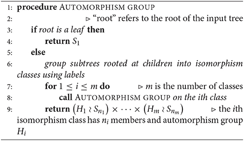
Algorithm 3 Compute the automorphism group of a rooted tree

FIGURE 3

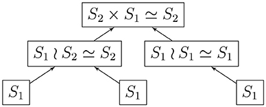
Figure 3. Computing the automorphism group of rooted tree 111010011000.

2.3.2. Automorphism Group of a Connected Component

Any connected component can be represented by a cyclic list of the in-trees of its directed cycle. For example, if there is a three-cycle in that component, with three different types of trees (say A, B, and C) attached to the cycle vertices in that order, then our cyclic list is ℓ = ABC = BCA = CAB. An in-tree consisting of a root • only will be denoted by E.

Theorem 6. If ℓ consists of a_i copies of a tree T_i for 1 ≤ i ≤ k and represents a connected component, where the prime block of ℓ is repeated s times, then the automorphism group of the component is

${\mathbb{Z}}_s\times {\displaystyle \prod _{i=1}^k{\displaystyle \prod _{j=1}^{a_i}Aut}}(T_i),withorders{\displaystyle \prod _{i=1}^k|}Aut(T_i){|}^{a_i}.$

The justification is based on the facts that prime blocks can only move cyclically, and that isomorphic but distinct trees within a block cannot be mapped to one another (roots in a block have to be mapped to roots in some block in the same order, with their in-trees attached).

Example 3. (a) A pure 3-cycle is given by the cyclic list EEE, with stabilizer ℤ₃ (r = s = 3). The automorphism group of each in-tree is the trivial group S₁, and the automorphism group of the directed 3-cycle is

${\mathbb{Z}}_3\times S_1\times S_1\times S_1\simeq {\mathbb{Z}}_3.$

(b) Let A be the in-tree • → •, and AEE be the list describing a component. Then the stabilizer of AEE is ℤ₁, and Aut(A) = S₁, giving us the automorphism group

${\mathbb{Z}}_1\times S_1\times S_1\times S_1\simeq {\mathbb{Z}}_1.$

(c) Let B be the in-tree • → • ← •. We have Aut(B) = S₂. Consider the component BEBE, with stabilizer ℤ₂ for the list. Then the automorphism group of the component is

${\mathbb{Z}}_2\times S_2\times S_1\times S_2\times S_1\simeq {\mathbb{Z}}_2\times {\mathbb{Z}}_2\times {\mathbb{Z}}_2.$

2.3.3. Automorphism Group of a Functional Digraph

Given the adjacency matrix of a functional digraph, we identify its connected components, directed cycles, and in-trees using Algorithm 1. Algorithm 2 codes the trees, which helps us sort them out. Algorithm 3 computes the automorphism groups of the distinct trees, and the algorithm described briefly in section 2.2.2 shows which cyclic lists corresponding to components are identical. Then we find the automorphism group of each distinct component using Theorem 6, and compute the overall group by Theorem 5.

2.4. The Entropy of a Functional Digraph

Defining a notion of entropy for any kind of “system” that has “states” is occasionally useful. The entropy of the directed graph of the states of a finite cellular automaton was considered by Wolfram [10]. He pointed out that entropy should be a measure of irreversibility –in case of a function, non-invertibility– and disorganization. For reasons to be discussed in section 6, we have chosen to define the entropy of a functional digraph G as the nonpositive and non-additive quantity

$S(G)=-\ln |\text{Aut}(G)|$

for any labeling of the vertices. The definition can be extended to any digraph. This way, S(G) has a maximum value of zero when G has maximum asymmetry: there are no authorized permutations of the vertices that leave the digraph invariant, and the automorphism group consists of the identity permutation.

Let G_j (1 ≤ j ≤ ν) denote the non-isomorphic connected components of a functional digraph G, n_j be the number of components of type G_j, C_j be the directed cycle in G_j, $T_i^{(j)}$ (1 ≤ i ≤ k^(j)) be the distinct in-trees attached to the cycle C_j, $a_i^{(j)}$ be the number of in-trees of type $T_i^{(j)}$, and s^(j) be the number of prime blocks in the cyclic list representing G_j. Hence, by Theorems 5 and 6, we have

$\begin{array}{l}S(G)=-{\displaystyle \sum _{j=1}^{\nu }{n}_j}\left[\ln s^{(j)}+{\displaystyle \sum _{i=1}^{k^{(j)}}{a}_i^{(j)}}\ln |\text{Aut}(T_i^{(j)})|\right]-{\displaystyle \sum _{j=1}^{\nu }\ln }(n_j!)\\ =\text{ }-\text{}{\displaystyle \sum _{j=1}^{\nu }{n}_j}\ln s^{(j)}-\text{}{\displaystyle \sum _{j=1}^{\nu }{\displaystyle \sum _{i=1}^{k^{(j)}}{n}_j}}{a}_i^{(j)}\ln |\text{Aut}(T_i^{(j)})|-\text{}{\displaystyle \sum _{j=1}^{\nu }\ln }(n_j!).\end{array}$

To summarize, the entropy of a functional digraph is the sum of the entropies of all constituent in-trees, plus correction factors for the rotational symmetries of prime blocks in cycles, and for the swapping of identical components of the digraph.

2.5. Algorithm for Functional Digraph Entropy

We may now compute the entropy of large functional digraphs without computing the automorphism group; the logarithms grow very slowly. Figure 4 shows the simultaneous coding and entropy computations for one rooted tree. The combined algorithm was implemented in Lua, which can run on many platforms without changes [2].

FIGURE 4

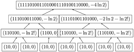
Figure 4. Computing (c, S), code and entropy of a rooted tree, simultaneously.

3. Introduction –Gene Regulatory Networks

3.1. Systems Biology, Modularity, and Gene Regulatory Networks

The idea of modularity in evo-devo, namely, that organisms are simply hierarchically arranged “quasi-independent parts that are tightly integrated within themselves” ([11]), is relatively new. Modern practitioners of biology by and large accept this dogma and deal in systems biology ([12, 13]), where “complex behaviors of biological systems emerge from the properties of the components and interactions in the systems” ([14]). We will introduce the systems-biological model of Boolean networks, in the particular case of GRNs, below. Two kinds of digraphs, wiring diagrams and phase spaces, are involved in the compositions of GRNs. Their adjacency matrices and spectra play an important role in describing the physical structure of the networks, which is the first direct link of linear algebra to biology. The second link is behavioral and involves the stability and adaptability of GRNs in terms of the symmetries (automorphism group) of their phase spaces, which, in turn, may be predicted by the entropy of these digraphs.

There are many directions of gene regulation in which a mathematician, biologist, or programmer may invest their efforts ([12, 13]), but we choose to study a generic, fully-known GRN and emphasize the usefulness of the universe of all possible deterministic successions of its collective states, a.k.a. the phase space. Although exponentially larger than the wiring diagram—a digraph showing which genes affect which, a structural simplicity makes the former more desirable over the latter, in our opinion, when computational complexity is taken out of the picture. A phase space is nothing but a digraph representation of a function on a finite set, and its sparse adjacency matrix as well as its computable entropy can reveal troves of information about real-life systems.

This fertile area of systems biology arguably originated in a 1969 article [15] by Stuart A. Kauffman, who was responsible for crystallizing notions such as (1) consistent cell types (phenotypes) are due to stable cycles in the phase space of GRNs, whereas cellular differentiation (adaptability) is the result of slight instability of same; (2) stability and adaptability of organisms may depend strongly on the connectivity of these networks as well as the rules of interaction between the components; and (3) biological evolution may well be the result of the interaction of self-organization with natural selection [15–17]. Kauffman experimentally studied the stability properties of large ensembles of random GRNs with selected parameters, and came to an interesting conclusion: regardless of the number n of genes, the average number k of incoming degrees for the wiring diagram was the decisive factor for whether the system was going to be stable, chaotic, or in between. In particular, k < 2 indicated stability, meaning mostly the states staying in the same small basin of attraction under a stochastic perturbation; k > 2 indicated chaotic behavior, e.g., having large, practically infinite, cycles; and k = 2 was just right, in that such systems exhibited a good balance between stability and adaptability, with some medium-size cycles. Without this balance, the existence and diversity of life would not have been possible. Kauffman [15, 16] convincingly argues via simulations and real-life observations that it is more plausible for nature to have initiated random connections in “metabolic nets” than not, and those that were successful had low connectivity and hence a delicate balance between stability and adaptability.

3.2. Structure and Examples of GRNs

Gene Regulatory Networks (GRNs) form a flexible modeling scheme for synthesizing and analyzing the interactions of clusters of up to thousands of factors such as functional genes, enzymes, and other proteins in a cell (all loosely called genes) that affect one another's function in a particular biological process, such as the successfully deciphered lac operon in Escherichia coli [18–20]. A GRN consists of a wiring diagram, which is a labeled digraph on n vertices (genes), where a directed edge indicates an influence of the gene at the initial vertex on the one at the terminal vertex. The nature of the combined influence of k genes on a fixed one is described by an update function of k variables for the target gene. The simplest GRN models make the fewest assumptions, namely, only ON/OFF states for the genes and synchronous deterministic updating of the states by Boolean update functions. Then the phase (state) space of the GRN –a functional digraph depicting all possible collective states and the deterministic transition rules of all genes– is neatly divided into connected components, each being the basin of attraction of a single dynamic attractor, or directed cycle. We contend that the adjacency matrices of phase spaces, which have been largely ignored in the GRN literature (with few exceptions), provide a rich source of information on the structure and properties of the whole system. For example, according to Wuensche [21], “[i]n the context of random Boolean networks of genetic regulatory networks, basins of attraction represent a kind of modular functionality, in that they allow alternative patterns of gene expression in the same genome, providing a mechanism for cell differentiation, stability, and adaptability.”

Example 4 (Wang et al. [14], Figure 1). Figure 5 shows a small wiring diagram of three genes, v₁, v₂, and v₃, where directed edges show nontrivial influences of the genes on one another. The update rule for gene v_i is given by the Boolean function f_i, where a variable x_j may take on the value 1 or 0 according to the active/inactive state of gene v_j, and the phase/state space shows the deterministic flow of the combined states of the genes. There are three basins of attraction, meaning that applying the rules to any combined initial state of the genes (possibly in the form of low/high concentrations of certain chemicals) causes the dynamics to be caught forever in one of the three directed cycles shown; two of them are loops and one is a two-cycle. The top (the wiring diagram and the Boolean update functions) and the bottom (the phase space) of Figure 5 are completely equivalent.

FIGURE 5

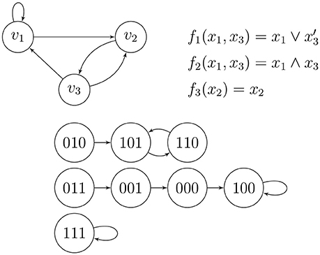
Figure 5. Two equivalent pictures of a gene regulatory network (GRN).

A Boolean function written in terms of logic operators can be converted into a polynomial over 𝔽₂ via the redundant dictionary x ∧ y = xy (AND), x ∨ y = x + y + xy (OR), x′ = 1 + x (NOT), and x ⊕ y = x + y (XOR). When these functions are written in simplest form, they contain no fictitious variables. The update functions f_i collectively determine a global update function F = (f₁, …, f_n) from ${𝔽}_2^n$ to ${𝔽}_2^n$.

Certain kinds of Boolean functions have emerged to play an important role in GRN theory via parallel works of biologists, mathematicians, and electrical engineers over decades, as summarized by He et al. [22] (also see [16]). A canalizing Boolean function is one that is non-constant and contains a dominant, canalizing variable x_i such that when x_i takes on a particular value, the function takes on a particular value. For example, f(x, y) = x ∧ y and f(x, y) = x ∨ y are both canalizing functions, each of which have x and y as canalizing variables. A nested canalizing function (NCF), called a unate cascade function by electrical engineers, is of the form

$f(x_1,\dots ,x_n)=y_1{\diamond }_1(y_2{\diamond }_2(\cdots (y_{n-1}{\diamond }_{n-1}{y}_n))\cdots ),$

where each y_i is either x_i or $x_i^{\prime }$, and each operation ◇_i is either ∧ or ∨. Apart from a certain economy of calculation (they have the shortest “average path lengths” for their binary decision diagrams among all other Boolean functions in the same number of variables; see [22]), or perhaps because of it, they are thought to be some of the best candidates for update functions in GRNs. Indeed, there are many known examples of NCFs in systems biology. Kauffman [15] showed that NCFs with average incoming degree k = 2 were best candidates for deterministic GRNs to become successful models. Note that the GRN in Example 4 and Figure 5 exhibits NCFs.

3.3. Computing the Matrix of the Phase Space

The N = 2ⁿ states in the phase space of a GRN on n genes are the vertices of a functional digraph. We can simply choose to convert the binary representations of the states (with n digits) to nonnegative integers, and add 1 to simplify the indexing of the adjacency matrix. Thus, 000 is 1, 001 is 2, 111 is 8, etc. That is, “row x₁ ⋯ x_n” has a 1 in “column F(x₁ ⋯ x_n).”

Example 5. We consider again the phase space of the three-gene GRN in Example 4 and Figure 5. Once we make the conversion from the binary labels of the vertices to decimal (plus one), we form the adjacency matrix

$A=\left(\begin{array}{llllllll}0\hfill & 0\hfill & 0\hfill & 0\hfill & 1\hfill & 0\hfill & 0\hfill & 0\hfill \\ 1\hfill & 0\hfill & 0\hfill & 0\hfill & 0\hfill & 0\hfill & 0\hfill & 0\hfill \\ 0\hfill & 0\hfill & 0\hfill & 0\hfill & 0\hfill & 1\hfill & 0\hfill & 0\hfill \\ 0\hfill & 1\hfill & 0\hfill & 0\hfill & 0\hfill & 0\hfill & 0\hfill & 0\hfill \\ 0\hfill & 0\hfill & 0\hfill & 0\hfill & 1\hfill & 0\hfill & 0\hfill & 0\hfill \\ 0\hfill & 0\hfill & 0\hfill & 0\hfill & 0\hfill & 0\hfill & 1\hfill & 0\hfill \\ 0\hfill & 0\hfill & 0\hfill & 0\hfill & 0\hfill & 1\hfill & 0\hfill & 0\hfill \\ 0\hfill & 0\hfill & 0\hfill & 0\hfill & 0\hfill & 0\hfill & 0\hfill & 1\hfill \end{array}\right).$

3.4. The Inverse Problem

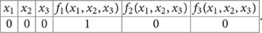
Conversely, every 2ⁿ × 2ⁿ matrix with exactly one 1 in every row and 0's elsewhere corresponds to a Boolean function $F:{𝔽}_2^n\to {𝔽}_2^n$ when we identify the rows and column indices with binary representations of 0 through 2ⁿ − 1: every functional digraph with 2ⁿ consecutively labeled vertices is the phase space of some GRN with update function F. We make a 2ⁿ × 2n table by filling out the left half with the digits of these binary numbers that correspond to the rows of A, and the right half with the digits of the binary numbers that correspond to the column for which that row has a 1 in A. For example, if n = 3 and the first row of the matrix has a 1 in the 5th column (↔ 100) as in Example 5, then the first row of the table will read

x₁0x₂0x₃0f₁(x₁, x₂, x₃)1f₂(x₁, x₂, x₃)0f₃(x₁, x₂, x₃₎0.

In short, this is the truth table of all n Boolean functions that act on the n labeled genes v₁, …, v_n.

4. Stability of GRNs

4.1. Old and New Definitions of Stability

We shall study the stability of the phase space of a GRN under stochastic perturbations, which are chance flips of bits (the on-off states) in the overall state of the wiring diagram. The definition of stability varies somewhat in the literature, but has about the same effect on the structure of the phase space. Kauffman [15] originally defined the stability of any one attractor (cycle) as the system's tendency to stay in the same basin after a minimal perturbation, that is, a chance flip of the state of any one of the genes. He also envisioned a series of such flips, which form a Markov process. In many other studies, stability is “characterized by whether small errors, or random external perturbations, tend to die out or propagate throughout the network” ([22]). The latter approach deals directly with the wiring diagram, and measures the spread of fluctuations, but not a priori whether such fluctuations result in an overall phase change from one basin to another. Following and expanding Kauffman, stability for us will mean a high probability of the GRN staying in the same basin of attraction of the phase space after any number of possible flips of individual gene-states in one time step, whereas instability will be indicated by a high probability of switching to another basin. Using our new tools, we will also define and compute the entropy of a GRN in terms of the group of automorphisms (in other words, the symmetry) of its phase space, showing strong correlations with stability: after all, the physical and information-theoretic definitions of entropy are measures of the disorder of the underlying micro-states of a system. Fast algorithms that compute the graph structure as well as the stability and entropy of a generic phase space from its adjacency matrix will be provided.

4.2. Computing Stability

Given a connected component with m states {s_u1, …, s_um} in the phase space of an n-gene GRN, we define the kth-order stability of the component to be the probability p_k that randomly flipping k bits in one randomly chosen state will produce another state in the same component, where 0 ≤ k ≤ n (clearly, p₀ = 1). This probability is equal to the number T_k of distinct ordered pairs (s_ui, s_uj) where flipping k bits of s_ui in arbitrary positions produces the state s_uj, divided by the number of all possible k-flips of all states, which is $m\left(\genfrac{}{}{0.0pt}{}{n}{k}\right)$ (note that T₀ = 0). We can compute all stabilities simultaneously by starting with the component's states by Algorithm 4, once the components have been characterized by Algorithm 1.

ALGORITHM 4

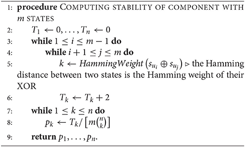
Algorithm 4 Stability of given connected component

Alternatively, since a GRN is expected to spend most of its time in cycle states, we may assume that only one of the cycle states will be affected. Let a and b be the numbers of cycle and transient states in the given component of m states respectively (a + b = m). We initialize all T_i to zero as before, and add 2 to T_k if the Hamming distance between two distinct cycle states is k and add 1 if the distance between a cycle state and a transient state is k. There are $\left(\genfrac{}{}{0.0pt}{}{a}{2}\right)$ unordered cycle pairs and ab mixed state pairs. After we compute the T_k, the k-stability for the component becomes $p_k=T_k/\left[a\left(\genfrac{}{}{0.0pt}{}{n}{k}\right)\right]$ (where T₀ = a).

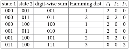
Example 6. Consider the phase space for the three-gene GRN in Example 4. We find the six unordered Hamming distances between the four states of the largest connected component, C:

We have T₁ = 6, T₂ = 4, and T₃ = 2 (these are the numbers of ordered pairs of states in C that differ by one, two, and three flips respectively.) Finally, we compute

$p_1=\frac{T_1}{|C|\left(\begin{array}{c}n\\ 1\end{array}\right)}=\frac{1}{2},p_2=\frac{T_2}{|C|\left(\begin{array}{c}n\\ 2\end{array}\right)}=\frac{1}{3},\text{ and }{p}_3=\frac{T_3}{|C|\left(\begin{array}{c}n\\ 3\end{array}\right)}=\frac{1}{2}.$

These are the probabilities that the component C will be mapped to itself after a flip of one, two, or three bits of a randomly chosen state respectively.

Hence, we may now construct the transition matrix P⁽¹⁾ of Kauffman [15], which gives us the probability that state s_i goes to state s_j after one flip of any one state in the whole phase space: $P_{ij}^{(1)}=P(s_i\mapsto s_j|\mathrm{\text{one flip}})$. There will be exactly n (1/n)'s in each row/column, and the rest of the N − n entries will be zero. This is a symmetric matrix since flipping is described as the addition of 1 = −1 to one digit in 𝔽₂. The matrix represents the linear transformation that sends each state to a weighted linear combination of its 1-neighbors in terms of Hamming distance. We can similarly construct matrices P^(k) for 1 ≤ k ≤ n, where k out of n bits in a state will be flipped: each row/column will contain $\left(\genfrac{}{}{0.0pt}{}{n}{k}\right)$ nonzero elements, all equal to $1/\left(\genfrac{}{}{0.0pt}{}{n}{k}\right)$. We define P⁽⁰⁾ = I; if no flips occur, then all states go to themselves with probability 1.

Let us fix a connected component C of the phase space. The jth column of P^(k), $P^{(k)}{e}_j$, multiplied by 1/|C|, represents the probability distribution for the k-flipped state s_j. We multiply the result on the left by $1_C^T$. The final operation adds up the probabilities that the state s_j will end up in component C. If we sum these numbers over all j for which s_j ∈ C, then we obtain the probability $p_k^C$ that a k-flip will result in C being mapped back to C:

$p_k^C=\frac{1}{\left|C\right|}{\displaystyle \sum _{s_j\in C}{\mathbf{1}}_C^T}{P}^{(k)}{e}_j=\frac{1}{\left|C\right|}{\mathbf{1}}_C^T{P}^{(k)}{\displaystyle \sum _{s_j\in C}{e}_j}=\frac{1}{\left|C\right|}{\mathbf{1}}_C^T{P}^{(k)}{\mathbf{1}}_C.$

If we want to switch to just starting with the cycle states, say C′ ⊆ C, then the vector 1_C on the right can be replaced by $1_{C^{\prime }}$. Using this formalism, we can apply flips with any probability distribution we like in a simulation.

Example 7. Let us repeat the computations in Example 6 with the matrix formulas. Once again, let C be the largest connected component of our phase space. The transition matrices for the whole phase space are

$P^{(1)}=\left(\begin{array}{cccccccc}0& 1/3& 1/3& 0& 1/3& 0& 0& 0\\ 1/3& 0& 0& 1/3& 0& 1/3& 0& 0\\ 1/3& 0& 0& 1/3& 0& 0& 1/3& 0\\ 0& 1/3& 1/3& 0& 0& 0& 0& 1/3\\ 1/3& 0& 0& 0& 0& 1/3& 1/3& 0\\ 0& 1/3& 0& 0& 1/3& 0& 0& 1/3\\ 0& 0& 1/3& 0& 1/3& 0& 0& 1/3\\ 0& 0& 0& 1/3& 0& 1/3& 1/3& 0\end{array}\right),$

$P^{(2)}=\left(\begin{array}{cccccccc}0& 0& 0& 1/3& 0& 1/3& 1/3& 0\\ 0& 0& 1/3& 0& 1/3& 0& 0& 1/3\\ 0& 1/3& 0& 0& 1/3& 0& 0& 1/3\\ 1/3& 0& 0& 0& 0& 1/3& 1/3& 0\\ 0& 1/3& 1/3& 0& 0& 0& 0& 1/3\\ 1/3& 0& 0& 1/3& 0& 0& 1/3& 0\\ 1/3& 0& 0& 1/3& 0& 1/3& 0& 0\\ 0& 1/3& 1/3& 0& 1/3& 0& 0& 0\end{array}\right),$

and

$P^{(3)}=\left(\begin{array}{cccccccc}0& 0& 0& 0& 0& 0& 0& 1\\ 0& 0& 0& 0& 0& 0& 1& 0\\ 0& 0& 0& 0& 0& 1& 0& 0\\ 0& 0& 0& 0& 1& 0& 0& 0\\ 0& 0& 0& 1& 0& 0& 0& 0\\ 0& 0& 1& 0& 0& 0& 0& 0\\ 0& 1& 0& 0& 0& 0& 0& 0\\ 1& 0& 0& 0& 0& 0& 0& 0\end{array}\right).$

The indicator vector of the component is 1_C = (1, 1, 0, 1, 1, 0, 0, 0)^T, and the k-stabilities of C for k = 1, 2, 3 are given by

$\begin{array}{l}{p}_1=\frac{1}{4}{\mathbf{1}}_C^T{P}^{(1)}{\mathbf{1}}_C=\frac{1}{2},p_2=\frac{1}{4}{\mathbf{1}}_C^T{P}^{(2)}{\mathbf{1}}_C=\frac{1}{3},p_3=\frac{1}{4}{\mathbf{1}}_C^T{P}^{(3)}{\mathbf{1}}_C\\ =\frac{1}{2}.\end{array}$

Next, we would like to define and compute the overall stability, p, of the connected component. Naturally, p is the probability that a randomly chosen state (alternatively, a cycle state) will stay in the component after a set of randomly chosen bits of it are flipped. We will assume here that each bit is flipped independently of the others with probability ϵ. This leads to the binomial distribution B(n, ϵ). Any other distribution on the number of bits can be similarly accommodated. This may be necessary as the “genes” are expected to be structurally and behaviorally different, unlike the statistical-mechanics situation with identical particles of gas. Given any state, the probability that k bits of it will be flipped is $\left(\genfrac{}{}{0.0pt}{}{n}{k}\right){ϵ}^k{(1-ϵ)}^k$. Then we have

$\begin{array}{l}p={\displaystyle \sum _{k=0}^n\left(\begin{array}{c}n\\ k\end{array}\right)}{ϵ}^k{\left(1-ϵ\right)}^k{p}_k={\displaystyle \sum _{k=0}^n\left(\begin{array}{c}n\\ k\end{array}\right)}{ϵ}^k{\left(1-ϵ\right)}^k\frac{T_k}{m\left(\begin{array}{c}n\\ k\end{array}\right)}\\ =\frac{1}{m}{\displaystyle \sum _{k=0}^n{ϵ}^k}{\left(1-ϵ\right)}^{n-k}{T}_k\end{array}$

if all states are targeted for flips, and

$p=\frac{1}{a}{\displaystyle \sum _{k=0}^n{ϵ}^k}{(1-ϵ)}^{n-k}{T}_k$

if only cycle states are targeted. Assume that there are ν connected components, with m⁽¹⁾, …, m^(ν) states each, and a⁽¹⁾, …, a^(ν) corresponding cycle states respectively. Let p⁽ⁱ⁾ denote the stability of the ith component computed as above. The individual stabilities will be weighted by the probability that a randomly chosen state will belong to that component, or alternatively, be a cycle state of that component. In the first case, we compute the stability of the phase space as

$P={\displaystyle \sum _{i=1}^{\nu }\frac{m^{(i)}}{2^n}}{p}^{(i)}=\frac{1}{2^n}{\displaystyle \sum _{i=1}^{\nu }{m}^{(i)}}{p}^{(i)}=\frac{1}{2^n}{\displaystyle \sum _{k=0}^n{ϵ}^k}{(1-ϵ)}^{n-k}{\displaystyle \sum _{i=1}^{\nu }{T}_k^{(i)}},$

and in the second case, as

$P={\displaystyle \sum _{i=1}^{\nu }\frac{a^{(i)}}{{\displaystyle \sum _{j=1}^{\nu }{a}^{(j)}}}}{p}^{(i)}=\frac{{\displaystyle \sum _{i=1}^{\nu }{a}^{(i)}}{p}^{(i)}}{{\displaystyle \sum _{j=1}^{\nu }{a}^{(j)}}}.$

5. Entropy of GRNs: a Comparison With Stability

5.1. Simulation

We fix N = 2ⁿ, the number of states in the phase space. There are a_N unlabeled non-isomorphic phase spaces, or different-shaped functions, given by the OEIS sequence A001372 [23]. Call these unlabeled digraphs D₁, …, D_aN. Let ${\left\{P(i)\right\}}_{i=1}^{a_N}$ be an arbitrary probability mass function. Define the entropy expectation of P to be

$H(P)={\displaystyle \sum _{i=1}^{a_N}P}(i)S(D_i),$

where S(D_i) is the entropy defined above. The neutral entropy expectation is defined to be

$\frac{N!}{N^N}{\displaystyle \sum _{i=1}^{a_N}S}(D_i)e^{S(D_i)}.$

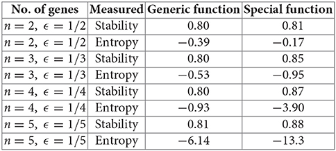
This is equivalent to the expectation for the probability mass function $p(i)=\left[N!/\left|\mathrm{\text{Aut}}(D_i)\right|\right]/N^N$ (see Lemma 3). For n = 2, 3, 4, 5, and using generic vs. nested canalizing Boolean update functions (section 3.2) with k = 2, we ran 100,000 simulations and averaged the stability and entropy values, as defined in this paper. The mean stability values were slightly higher with special update functions, in line with Kauffman's ideas [15, 16]. However, the mean entropy calculations were more interesting: for n = 3, 4, 5, we had a markedly lower value for entropy (hence, more order and symmetry) for special update functions, correlating with the higher stability. The difference got more prominent as n increased. Only the case n = 2, which is too small to be meaningful, was anomalous.

The Lua code created by the first author can be accessed at [2]. We hope that our modest results will lead to more ambitious simulations, start new theoretical discussions, and open new possibilities in experimental designs.

6. Concluding Remarks

There is a theoretical chasm in the current literature between the definition and practice of GRNs. As fewer vertices are needed, simulations of the wiring diagrams rather than the phase spaces is the norm, but the mathematical framework is somewhat incomplete. In contrast, a phase space gives us both the wiring diagram and the update function, and is much more tractable. In the words of Wuensche [21], when we look at the phase space,

High convergence implies order [high symmetry, low entropy] in space-time patterns: short, bushy, highly branching transient trees, with many leaves and small attractor periods. Conversely, low convergence implies chaos [low symmetry, high entropy] in space-time patterns: long, sparsely branching transient trees, with few leaves and long attractor periods.

Hence, we are justified in considering the digraph symmetries of the phase space as a measure of convergence and stability.

It may eventually be possible to bridge the theory gap between definitions and simulation results for biological phase spaces, and analytically demonstrate the relationships among the connectivity of the wiring space, and the stability, symmetry, and entropy of the phase space. Systems biology and evolutionary theory would benefit from such a solid foundation.

Moreover, mathematicians should appreciate functional digraphs and their automorphism groups and entropies in their own right, with a concrete algorithm to compute the latter objects. It would also be worthwhile to shift the focus of algebraic graph theory from undirected graphs to digraphs, from static configurations to dynamic ones, and from the spectral properties of Laplacians (usually associated with undirected graphs) to those of the adjacency matrices of digraphs: although tournament scheduling will never go out of fashion, dynamical and directed networks such as GRNs and the Internet are increasingly more important in real-world problems.

7. Author Contributions

FA is the author who initiated the study, made spectral computations, did most of the writing and editing, and researched existing literature on GRNs. Contributions from both authors were substantial and collaborative. DA is an undergraduate computer science and mathematics major at UIUC, with prior experience in publishing and presenting academic work. His contributions have been theoretical as well as computational. DA was the one who suggested the new definitions of entropy and stability, as well as methods of computing automorphism groups, and has done all the coding.

Conflict of Interest Statement

The authors declare that the research was conducted in the absence of any commercial or financial relationships that could be construed as a potential conflict of interest.

Footnotes

1. ^Contrast with Harary et al. [1], Chapter 5.

References

1. Harary F, Norman RZ, Cartwright D. Structural Models: An Introduction to the Theory of Directed Graphs. New York, NY: Wiley (1965).

Google Scholar

2. Akman D. Available online at: https://github.com/GeneRegulatoryNetworks/Algorithms

3. Wuensche A. The ghost in the machine: basins of attraction of random Boolean networks. In: Langton CG, editor. Artificial Life III. Santa Fe Institute Studies in the Sciences of Complexity; Reading, MA: Addison-Wesley (1994). p. 465–501.

Google Scholar

4. Rotman JJ. An Introduction to the Theory of Groups, Graduate Texts in Mathematics. 4th ed. New York, NY: Springer (1994).

5. Jordan C. Sur les assemblages de lignes. J Reine Angew Math. (1869) 70:185–90.

Google Scholar

6. Read RC. The coding of various kinds of unlabeled trees. In: Read RC, editor. Graph Theory and Computing. New York, NY: Academic Press (1972). p. 153–82.

Google Scholar

7. Knuth D, Morris JH, Pratt V. Fast pattern matching in strings. SIAM J Comput. (1977) 6:323–350. doi: 10.1137/0206024

CrossRef Full Text | Google Scholar

8. Shiolach Y. Fast canonization of circular strings. J Algorithms (1981) 2:107–121.

9. Chen KT, Fox RH, Lyndon RC. Free differential calculus IV: the quotient groups of the lower central series. Ann Math. (1958) 68:81–95.

Google Scholar

10. Wolfram S. Statistical mechanics of cellular automata. Rev Modern Phys. (1983) 55:601–44.

Google Scholar

11. Schlosser G, Wagner GP. Chapter 1: Introduction: the modularity concept in developmental and evolutionary biology. In: Schlosser G, Wagner GP, editors. Modularity in Development and Evolution. Chicago, IL: Chicago University Press (2004). p. 1–11.

Google Scholar

12. Breitling R. What is systems biology? Front Physiol. (2010) 1:9. doi: 10.3389/fphys.2010.00009

PubMed Abstract | CrossRef Full Text | Google Scholar

13. Ideker T, Galitski T, Hood L. A new approach to decoding life: systems biology. Annu Rev Genomics Hum Genet. (2001) 2:343–72. doi: 10.1146/annurev.genom.2.1.343

PubMed Abstract | CrossRef Full Text | Google Scholar

14. Wang RS, Saadatpour A, Albert R. Boolean modeling in systems biology: an overview of methodology and applications. Phys Biol. (2012) 9:055001. doi: 10.1088/1478-3975/9/5/055001

PubMed Abstract | CrossRef Full Text | Google Scholar

15. Kauffman SA. Metabolic stability and epigenesis in randomly constructed genetic nets. J Theor Biol. (1969) 22:437–67.

PubMed Abstract | Google Scholar

16. Kauffman SA. The Origins of Order: Self-Organization and Selection in Evolution. New York, NY: Oxford University Press (1993).

Google Scholar

17. Kauffman SA. Antichaos and adaptation. Sci Am. (1991) 265:78–84.

PubMed Abstract | Google Scholar

18. Jacob F, Monod J. Genetic regulatory mechanisms in the synthesis of proteins. J Mol Biol. (1961) 3:318–56.

PubMed Abstract | Google Scholar

19. Laubenbacher R, Sturmfels B. Computer algebra in systems biology. Amer Math Monthly (2009) 116:882–891. doi: 10.4169/000298909X477005

CrossRef Full Text | Google Scholar

20. Robeva R, Kirkwood B, Davies R. Chapter 1: Mechanisms of gene regulation: Boolean network models of the lactose operon in Escherichia coli. In: Robeva R, Hodge T. editors. Mathematical Concepts and Methods in Modern Biology: Using Modern Discrete Models. Amsterdam: Academic Press (2013). p. 1–35.

21. Wuensche A. Chapter 13: Basins of attraction in network dynamics: a conceptual framework for biomolecular networks. In: Schlosser G, Wagner GP, editors. Modularity in Development and Evolution. Chicago, IL: Chicago University Press (2004). 288–311.

Google Scholar

22. He Q, Macauley M, Davies R. Chapter 5: Dynamics of complex boolean networks: canalization, stability, and criticality. In: Robeva R, editor. Algebraic and Discrete Methods for Modern Biology. Amsterdam: Academic Press (2015). p. 93–119.

Google Scholar

23. The Online Encyclopedia of Integer Sequences. Available online at: https://oeis.org