A Comparison of the Single, Conditional and Person-Specific Standard Error of Measurement: What do They Measure and When to Use Them?

Introduction

Within the Classical Test Theory (CTT), the Standard Error of measurement (SEm; [1]) is often used as an expression of (un)certainty of test results in education, psychological assessment and health related research. Tests based on CTT usually report the traditional “single” SEm, which briefly works as follows. The test is administered once to a group of persons from the desired population (i.e., the “norm population”) and one CTT-based SEm is estimated for all future examinees, hence the term “single” [1–4]. Another possibility is the estimation of a person-specific SEm, which is calculated—as the name implies—for every examinee separately. This person-specific SEm is usually seen as an intermediate step in the estimation of the conditional SEm (see [5]), but as we show it can also be used on its own. When the expected value is taken of the person-specific SEm over all examinees with the same (expected) “true” test score, it yields a SEm for every group of examinees separately called the conditional SEm (see, for instance, [5]).

The choice for either of the three SEms depends on the assumptions that each of these SEms make about measurement (un)certainty. The single SEm, for instance, can only be used when two strict assumptions are met [6]. First, all persons must be measured with the same accuracy; i.e., the measurement error variance must be constant. Second, the person's intra-individual variation in measurements must equal the inter-individual variation in measurement of the norm-population examinees; i.e., intra-individual variation and inter-individual variation must be interchangeable [7]. Multiple authors have questioned the reasonableness of these assumptions. Sijtsma [8], for instance, writes: “… there is no reason whatsoever to assume that the propensity distributions of different persons must be identical to one another and to the between-person distribution based on single-administration data” (p. 118). With “propensity distribution” Sijtsma [8] refers to the hypothetical distribution of repeated measurements of single examinees. When picturing a class of—in many aspects—different examinees, it is hard to imagine that the test result of each of these examinees is governed by the same underlying propensity distribution. Furthermore, it seems unlikely that these propensity distributions equal an aggregated, between-person distribution calculated on the basis of a single test take. Molenaar [6] concludes: “(CTT) gives rise to serious questions regarding its applicability to individual assessment” (p. 203, also see [7]).

The two assumptions are relaxed when we move from the single to the conditional SEm. Instead of constant measurement error variance, the conditional SEm is based on the more lenient assumption of homogeneous measurement error variance (see [9]). This assumption states that measurement error variance is constant conditional on “true” test score. Thus, measurement error variance is only assumed constant for examinees with the same, underlying “true” test score. The same holds for the second assumption; only within a group of examinees with the same “true” test score, intra-individual variation and inter-individual variation in measurement are assumed interchangeable. Finally, a move from the conditional to the person-specific SEm leads to a drop of both assumptions altogether.

Based on the assumptions above, one might be inclined to opt for a conditional SEm or even for a person-specific one. However, there is no free lunch. The increasingly lenient assumptions with respect to measurement (un)certainty are accompanied by increasingly stricter assumptions with respect to the structure of a test and its items (we illustrate this in the next sections). Furthermore, there is a trade-off between the unbiasedness of SEm-estimates and their estimation variability. For instance, if examinees have their own unique measurement (un)certainty, the person-specific SEm will provide us with an unbiased estimate at the cost of being the most variable estimate of SEm.

Conventionally, CTT test makers and test users have “blindly” adopted the single SEm for individual inferences. We propose to not base this decision on convention, but on a deliberate consideration of characteristics of the test, its norm population and assumptions one is willing to make and their influence on the trade-off between unbiasedness and estimation variance. To aid this deliberate consideration, this paper first discusses the Classical Test Theory and how the single SEm, the person-specific SEm and the conditional SEm fit in this framework. In this discussion, differences in the estimation of the three SEms are shown and underlying assumptions are highlighted. Then, we zoom in on the trade-off between unbiasedness and estimation variance of the three SEms, which is followed by a simulation study. In this simulation study, we investigate how characteristics of the test and its norm population (i.e., number of repeated test takes, number of items, overall reliability, divisibility in parallel test parts, anticipated relationship between true test score and SEm and whether the scores are continuous or rounded and truncated) influence the trade-off between unbiasedness and estimation variance. Based on this simulation study, we end with a set of practical recommendations when to use each of the SEms.

Classical Test Theory

Throughout this paper, we built on the ideas and notation of Classical Test Theory¹ (CTT; [1–4]). CTT comprises a set of assumptions and conceptualizations that make it possible to model measurement error [4, 11]. In this section, we discuss the fundamentals of CTT. In the next section, we discuss how respectively the single Standard Error of measurement (SEm), the person-specific SEm and the conditional SEm fit within this CTT framework.

In essence, CTT assumes that every person has a “true” overall test score. This “true” overall test score is assumed to be time invariant. The difference between the fixed “true” score and the score obtained on a measurement is considered random measurement error:

$\begin{array}{rc}{e}_{gi}={\tau }_i-x_{gi}.& (1)\end{array}$

In Equation 1, e_gi denotes person's i measurement error on measurement occasion g. τ_i refers to the person's “true”, overall test score and x_gi to person's i obtained score on measurement occasion g. For this equation to hold, CTT assumes that person i is part of a well-defined population of persons ℘ (i ∈ ℘) and that the specific test, let's call this test a, is part of a well-defined set of possible tests ℜ (a ∈ ℜ).

Assume we can repeat the measurement of person i with test a many times independently. In that case, the random variable $E_{{}^{*}i}$ would contain all measurement errors e_gi of person i over G repeated measurements and the random variable $X_{{}^{*}i}$ would contain all observed scores x_gi of person i over G repeated measurements. Note the replacement of g with an asterisk to denote random measurements. τ_i in Equation 1 can then be conceptualized as the expected value of $X_{{}^{*}i}$:

$\begin{array}{rc}{\tau }_i={\text{E}}_i\left[X_{{}^{*}i}\right].& (2)\end{array}$

Since the expected value of x_gi equals τ_i, the expected value of $E_{{}^{*}i}$ is zero:

$\begin{array}{rc}{\text{E}}_i\left[E_{{}^{*}i}\right]=0,& (3)\end{array}$

where $E_{{}^{*}i}$ is expected to be normally distributed with finite variance σ²($E_{{}^{*}i}$):²

$\begin{array}{rc}{E}_{{}^{*}i}~N(0,{\sigma }^2(E_{{}^{*}i})),& (4)\end{array}$

where σ²($E_{{}^{*}i}$) here refers to intra-individual variation. Although Equations 1–4 are useful for the conceptualization of the conditional and the person-specific standard error of measurement later, they are not generally the focus of CTT [9]. Rather, CTT shifts the focus from the repeated measurement of a single, specific examinee to the single measurement of repeatedly, randomly selected examinees [1, 12]. Given that Equation 1 holds for a specific examinee i, it also holds for any randomly selected examinee. Therefore, if we denote the error random variable over randomly selected examinees by $E_{g^{*}}$, the true score random variable by $T_{{}^{*}}$ and the observed score random variable by $X_{g^{*}}$,

$\begin{array}{rc}{E}_{g^{*}}=T_{{}^{*}}-X_{g^{*}}& (5)\end{array}$

in ℘ or any subpopulation of ℘ (note the substitution of i by * to denote randomly selected examinees). Again, $E_{g^{*}}$ is expected to be normally distributed with finite variance σ²($E_{g^{*}}$):

$\begin{array}{rc}{E}_{g^{*}}~N(0,{\sigma }^2(E_{g^{*}})),& (6)\end{array}$

where σ²($E_{g^{*}}$) refers to inter-individual variation. As we explain in the coming sections, σ²($E_{g^{*}}$) in Equation 6 forms the basis for the single SEm while σ²($E_{{}^{*}i}$) from Equation 4 is crucial to the conditional and person-specific SEm.

Single Standard Error of Measurement

Definition

The single standard error of measurement, abbreviated here as single SEm, is defined as $\sqrt{{\sigma }^2(E_{g^{*}})}$; the square root of the variance in measurement errors of randomly selected examinees (see Equation 6). Because of the linear relationship in Equation 5 and zero correlation between $E_{g^{*}}$ and $T_{{}^{*}}$, the variance in measurement errors of randomly selected examinees is simply the difference between the total variation in observed scores and true-score variance (for proof see [9]):

$\begin{array}{rc}{\sigma }^2(E_{g^{*}})={\sigma }^2(X_{g^{*}})-{\sigma }^2(T_{{}^{*}}).& (7)\end{array}$

Estimation

As mentioned in the introduction, the single SEm is estimated based on a norm population. Since this norm population is only tested once, the true-score variance σ²(T*) is unknown and the single SEm cannot be estimated directly using Equation 7. In order to estimate σ²(E_g*), and eventually $\sqrt{{\sigma }^2(E_{g^{*}})}$, the unobservable quantity σ²(T*) must be rewritten in a potentially observable quantity. CTT does this by splitting the single measurement of the norm population into two parallel parts. “Parallel” means that the items and/or scores in the parts have the same underlying true score variable $T_{{}^{*}}$ and experimentally independent errors with equal variance σ²(E_g*) in ℘ and every subpopulation of ℘ (see definition 2.13.4, [1]). “Experimentally independent” (definition 2.10.1; [1]) implies that the correlation between errors of the parts equals zero. From a practical point of view, parallel test parts can be constructed by matching item content and item characteristics over parts. Examples of such item characteristics are item difficulty—the proportion of persons of the norm population answering the item correctly—and the reliability index, which is the point-biserial correlation between item and total score multiplied by the item standard deviation. Thus, even though items in a test are likely to differ in terms of difficulty and reliability, the idea is to group them in such a way that the groups of items (the parallel test parts) are comparable. An example of an algorithm capable of grouping items in an optimal way can be found in Sanders and Verschoor [14]. In the remainder of this article, we use K to denote the number of parallel test parts and k to refer to a specific parallel part. Multiple coefficients exist based on the correlation between K parallel measurements, such as the Spearman-Brown split half coefficient [15, 16]. These coefficients, here denoted by ${\rho }_{X{X}^{\prime }}$, are meant to estimate the reliability of the test, i.e., the ratio $\frac{{\sigma }^2(T_{{}^{*}})}{{\sigma }^2(X_{g^{*}})}$ (see [1]) adjusting for the change in test length and hence the single SEm can be estimated using:

$\begin{array}{r}{\sigma }^2(E_{g^{*}})={\sigma }^2(X_{g^{*}})-{\sigma }^2(T_{{}^{*}})={\sigma }^2(X_{g^{*}})-{\sigma }^2(X_{g^{*}})\frac{{\sigma }^2(T_{{}^{*}})}{{\sigma }^2(X_{g^{*}})}\\ ={\sigma }^2(X_{g^{*}})(1-{\rho }_{X{X}^{\prime }}).& (8)\end{array}$

In the remainder, we will use the Spearman-Brown split half coefficient (Equation 8). Note, however, that alternatives exist for the estimation of reliability that are based on more lenient assumptions of parallelism. Test halves can, for instance, be tau-equivalent, meaning that the true scores in both test parts are allowed to differ by a constant (equal for all examinees) and that their error variances are allowed to differ as well [17, 18] (also see [19] for an overview of reliability coefficients and their assumptions of parallelism). From a practical point of view, items in tau-equivalent test parts do not have to be matched as strictly on item characteristics such as item difficulty as is the case for parallel test parts.

Person-Specific Standard Error of Measurement

Definition

Whereas the single SEm is based on the variance in measurement errors of randomly selected examinees σ²(E_g*), see Equation 6, the person-specific SEm can be expressed as $\sqrt{{\sigma }^2(E_{{}^{*}i})}$; the square root of the variance in person i's measurement errors over repeated measurements (see Equation 4). As shown by Lord and Novick [1], the single SEm and the person-specific SEm are related to one another:

$\begin{array}{rc}{\sigma }^2(E_{g^{*}})=E\left[{\sigma }^2(E_{{}^{*}i})\right],& (9)\end{array}$

indicating that the between person variance on which the single SEm is based, is equal to the expected value of the within person error variance on which the person-specific error variance is based ([1]; p. 35; for a graphical illustration see our Figure 1). In other words, the single SEm $\sqrt{{\sigma }^2(E_{g^{*}})}$is the mean standard error of measurement in ℘ [1]. Estimating $\sqrt{{\sigma }^2(E_{{}^{*}i})}$ for every person separately thus leads to a correct estimate of $\sqrt{{\sigma }^2(E_{g^{*}})}$on average while allowing the possibility that some persons' measurements are inherently more consistent than others. Equation 9 shows that it is possible to aggregate σ²(E*_i) on the level of specific examinees to reach an estimate of σ²(E_g*) on a population level, but not the other way around. Thus, if we want to use σ²(E_g*), on which the single SEm is based, to make inferences on an individual level, we need to assume that (1) every examinee has the same error variance σ²(E_g*) and that this error variance equals σ²(E_g*); the assumptions of constant measurement error and interchangeability of intra-individual and inter-individual variation discussed previously.

FIGURE 1

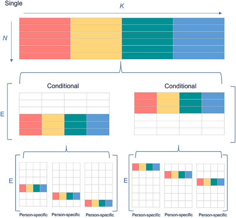
Figure 1. Illustration of the relationship between the single, conditional and person-specific standard error of measurement. The rows symbolize examinees N and the columns parallel parts K. The different colors indicate different test scores for the K parallel parts. E[] refers to the expectation over the variances between the brackets.

Estimation

Just as with the single SEm, the estimation of the person-specific SEm is based on splitting the test in parallel test parts. When a test is administered multiple times, the person-specific SEm can be estimated based on the variances within parallel test parts, σ²(X*_ki), operationalized as $\frac{{\displaystyle \sum _{g=1}^G}{(x_{gki}-{\bar{x}}_{*ki})}^2}{G-1}$where ${\bar{x}}_{*ki}$ denotes the mean of the kth parallel test part. Since the overall test score x_gi is the sum over (let's for simplicity assume unit-weighted) scores for each of the parallel parts, the error variance of x_gi can be expressed as [1]:

$\begin{array}{l}{\sigma }^2(E_{{}^{*}i})={\sigma }^2(X_{{}^{*}i})={\sum }_{k=1}^K{\sigma }^2(X_{{}^{*}ki})\\ +2{\sum }_{k<p}{\sigma }^2(X_{{}^{*}ki},X_{{}^{*}pi})& (10\text{a})\end{array}$

$\begin{array}{rc}{\sigma }^2(E_{{}^{*}i})={\sigma }^2(X_{{}^{*}i})={\sum }_{k=1}^K{\sigma }^2(X_{{}^{*}ki}).& (10\text{b})\end{array}$

In other words, the variance of the composite test score x_gi, and thus σ²(E*_i), is a function of the (unit-weighted) within variances of the parallel parts and their covariance. Since the parallel parts are experimentally independent, these covariances equal zero (Equation 10b, see Hu et al. [20] for the estimation of the person-specific SEm in the context of many repeated measurements).

As stressed in Sijtsma [8], there generally is a “… practical impossibility to administer the same test to the same individuals repeatedly – even twice is nearly impossible” (p. 117). Therefore, Equation 10 must be modified to accommodate a situation with only one test take. This is done by replacing the within parallel parts variances, ${\sigma }^2(X_{*ki})$, with the variance between parallel parts, ${\sigma }^2(X_{g*i})$:

$\begin{array}{rc}{\sigma }^2(E_{{}^{*}i})={\sigma }^2(X_{{}^{*}i})={\sum }_{k=1}^K{\sigma }^2(X_{g^{*}i})=K{\sigma }^2(X_{g^{*}i}).& (11)\end{array}$

This replacement is justified since, if we operationalize the variance between parallel parts as $\frac{{\displaystyle \sum _{k=1}^K}{(x_{gki}-{\bar{x}}_{g*i})}^2}{K-1}$where ${\bar{x}}_{g*i}$ denotes the mean of the gth measurement, the expected value of this between variance equals the expected value of the parallel parts' within variance, calculated across repeated measures:

$\begin{array}{rc}{\text{E}}_i\left[{\sigma }^2(X_{*ki})\right]={\text{E}}_i\left[{\sigma }^2(X_{g*i})\right]& (12)\end{array}$

The proof for this is straightforward:

$\begin{array}{l}{\text{E}}_i\left[K{\sigma }^2(X_{g*i})\right]=K{\text{E}}_i\left[\frac{{\displaystyle \sum _{k=1}^K}{(x_{gki}-{\overline{x}}_{g*i})}^2}{K-1}\right]\\ =K\frac{{\displaystyle \sum _{g=1}^G}\frac{{\displaystyle \sum _{k=1}^K}{(x_{gki}-{\overline{x}}_{g*i})}^2}{K-1}}{G-1}\end{array}$

and

$\begin{array}{l}{\text{E}}_i\left[K{\sigma }^2(X_{*ki})\right]=K{\text{E}}_i\left[\frac{{\displaystyle \sum _{g=1}^G}{(x_{gki}-{\overline{x}}_{*ki})}^2}{G-1}\right]=K\frac{{\displaystyle \sum _{k=1}^K}\frac{{\displaystyle \sum _{g=1}^G}{(x_{gki}-{\overline{x}}_{*ki})}^2}{G-1}}{K-1}\end{array}$

In other words, the expected variance between and within parallel parts is the same ■.

For normally distributed parallel measurements, the between variance σ²(X_g*i) is known to follow a scaled chi-squared distribution (see [21])³. Therefore, the between variance σ²(X_1*i) at a specific test take can also be perceived as a random sample of the scaled chi-squared distribution of a fixed, unknown ${\sigma }^2(E_{{}^{*}i})$ of person i.

Conditional Standard Error of Measurement

Definition

Just as the person-specific SEm, the conditional SEm is based on Equation 4. This conditional SEm can simply be expressed as the expected value of the person-specific SEms of examinees belonging to the same group j:

$\begin{array}{rc}{{\sigma }_{i\in j}(E_{{}^{*}i})=\sqrt{{{\text{E}}_{i\in j}}_{}\left[{\sigma }^2(E_{{}^{*}i})\right]}}_{}.& (13)\end{array}$

Ideally, every examinee in group j has the same “true” test score. Since examinee's “true” scores are unknown, they are typically grouped according to their total test scores⁴. Building on Equation 9, the relationship between the conditional and the single SEm can be described as follows (for a graphical illustration see Figure 1):

$\begin{array}{rc}{\sigma }^2(E_{g^{*}})={\text{E}}_{}\left[{\sigma }_{i\in j}^2(E_{{}^{*}i})\right],& (14)\end{array}$

that is, when we take the expected value over all the error variances in groups j, we find the between person variance on which the single SEm is based. Estimating ${\sigma }_{i\in j}^2(E_{{}^{*}i})$ for every group separately thus leads to a correct mean estimate of ${\sigma }^2(E_{g^{*}})$while allowing the possibility that low-scoring, average-scoring and/or high-scoring examinees have measurements that are inherently more or less consistent. Equation 13 shows that whereas the conditional SEm can be estimated by aggregating the person-specific SEms, it does not work the other way around. Thus, if we want to use ${\sigma }_{i\in j}^2(E_{{}^{*}i})$, on which the conditional SEm is based, to make inferences on an individual level, we need to assume that every examinee within group j has the same error variance; this is the homogeneous measurement error variance assumption discussed previously.

Estimation

Many procedures have been proposed in the literature to estimate the conditional SEm, including but not restricted to the binomial procedure [23], the compound binomial procedure [23] the Feldt-Qualls procedure ([25]; for a comparison of this procedure and the procedures previously mentioned see [26]), the item response theory procedure by Wang et al. [27] and the bootstrap procedure advocated by Colton et al. [28]. In the present article, we focus on the Feldt and Qualls [5] procedure, since this procedure is very similar to the procedure for estimating the person-specific SEm discussed previously. The Feldt and Qualls [5] procedure extends the original method proposed by Thorndike [29], where a test is split in two parallel halves. Thorndike [29] showed that the difference between two half-test scores equals the difference between their two errors (up to a constant, when the half tests are essentially tau-equivalent instead of classically parallel). With the assumption that the two errors are independent, the variance of the difference between the two half-test scores equals the error variance we are interested in. Feldt and Qualls [5] generalize this finding of Thorndike [29] to a situation with more than two parallel (or essentially tau-equivalent) parts:

$\begin{array}{rc}{\sigma }^2(E_{{}^{*}i})=K\left[\frac{{\displaystyle {\sum }_{k=1}^K}{(x_{gki}-{\overline{x}}_{g^{*}i})}^2}{K-1}\right],& (15)\end{array}$

where K in Equation 15 corrects for test length. That is, since the division of tests in parallel parts shortens the test by a factor K, we multiply by K to obtain an estimate for tests with the original test length [5]. Note that Equation 15 is equal to Equation 11 discussed earlier. To obtain the conditional SEm, the expected value needs to be taken over the result in Equation 15 for all examinees in a certain group j. The person-specific SEm can thus also be perceived as a special case of the conditional SEm when n_j = 1:

$\begin{array}{rc}{\sigma }_{i\in j}^2({\text{E}}_{{}^{*}i})=E_{i\in j}\langle K\left[\frac{{\displaystyle \sum _{k=1}^K}{\left(x_{gki}-{\overline{x}}_{g^{*}i}\right)}^2}{K-1}\right]\rangle .& (16)\end{array}$

When the parts are (essentially) tau-equivalent instead of classically parallel, Equation 15 can be replaced with:

$\begin{array}{rc}{\sigma }^2(E_{{}^{*}i})=K\left[\frac{{\displaystyle \sum _{k=1}^K}{\left(\left[x_{gki}-{\overline{x}}_{g^{*}i}\right]-\left[{\overline{x}}_{g^{*}i}-{\overline{x}}_{g^{**}}\right]\right)}^2}{K-1}\right]& (17)\end{array}$

where the part $\left[{\overline{x}}_{g^{*}i}-{\overline{x}}_{g^{**}}\right]$ accounts for differences in means of the parallel parts (${\overline{x}}_{g^{**}}$ denotes the “grand” mean over all parallel test parts) for the person-specific SEm with n_j = 1 and Equation 16 can be replaced with:

$\begin{array}{rc}{\sigma }_{i\in j}^2(E_{{}^{*}i})={\text{E}}_{i\in j}\langle K\left[\frac{{\displaystyle \sum _{k=1}^K}{\left(\left[X_{gki}-{\overline{X}}_{g^{*}i}\right]-\left[{\overline{X}}_{g^{*}i}-{\overline{X}}_{g^{**}}\right]\right)}^2}{K-1}\right]\rangle & (18)\end{array}$

for the conditional SEm with n_j > 1.

Bias-Variance Trade-Off

Ultimately, we want the estimate of SEm to be as reflective of the examinee's error variation as possible. Keeping in mind that the examinee is tested once, there are two factors that influence the adequacy of the estimated SEm for the examinee: (1) the (un)biasedness of the estimate and (2) its estimation variance.

Variance

Looking at the variance first, the following (in)equalities are at play:

$\begin{array}{c}Rule1.varianc{e}_{single}\le varianc{e}_{conditional}\le varianc{e}_{person-specific}\end{array}$

The justification for this rule is as follows. As discussed before, the variance between parallel parts of a person follows a scaled chi-squared distribution. The variance of this distribution equals:

$\begin{array}{ll}{\sigma }^2\left({\sigma }^2\left(X_{g*i}\right)\right)=\frac{2{\left({\text{E}}_i\left[{\sigma }^2\left(X_{g*i}\right)\right]\right)}^2}{K-1}.& (19)\end{array}$

Since the estimate of the person-specific error variance ${\sigma }^2(E_{{}^{*}i})$ simply follows by multiplying σ²(X_g*i) by K (see Equation 11), the estimation variance of ${\sigma }^2(E_{{}^{*}i})$ is:

$\begin{array}{rc}{\sigma }^2({\sigma }^2(E_{*i}))=K^2{\sigma }^2({\sigma }^2(X_{g*i}))& (20)\end{array}$

(see Feldt and Qualls [5]). By rules of error propagation, we know that the variance of n_j independent examinees equals $\frac{\sum _i{\sigma }^2({\sigma }^2(E_{{}^{*}i}))}{{n_j}^2}$ and thus the variance of the conditional SEm can be expressed as:

$\begin{array}{rc}{\sigma }^2\left({\sigma }_{i\in j}^2(E_{{}^{*}i})\right)=\frac{{\displaystyle {\sum }_i}{K}^2{\sigma }^2({\sigma }^2(X_{g^{*}i}))}{{n_j}^2}.& (21)\end{array}$

The variance of the conditional SEm thus also depends on the size of groups the J groups. Finally, since the single error variance ${\sigma }^2\left(E_{g^{\ast }}\right)=E_{}[{\sigma }^2\left(E{\ast }_i\right)]$ is usually computed for all future examinees, it is a constant and therefore its variance equals zero:

$\begin{array}{rc}{\sigma }^2({\sigma }^2(E_{g^{*}}))=0.& (22)\end{array}$

Comparing Equations 21 and 22, we see that Equation 21 can only equal Equation 22 when the numerator of Equation 21 results in zero. Since K² cannot equal zero (K has to be at least 2), the expression ${\sigma }^2({\sigma }^2(X_{g^{*}i}))$ has to become zero, which means that there is no variation in the between variances ${\sigma }^2(X_{g^{*}i})$. When this is true, also Equation 20 results in zero, explaining why the conditional and person-specific estimation variances are larger or equal to the estimation variance of the single SEm. On top of the situation in which ${\sigma }^2({\sigma }^2(X_{g^{*}i}))=0$, Equation 20 and 21 result in the same value when n_j = 1 (in this case, Equation 21 simplifies into Equation 20). In other instances, the person-specific SEm always exceeds the estimation variance of the conditional SEm.

Figure 2 illustrates Rule 1 graphically (see the R file “Figure 2.R” on the OSF page https://osf.io/6km3z/ for detailed information about this plot). The flat, mint colored surface shows the estimation variance of the single SEm and the tilted vertical surface illustrates the estimation variance of the person-specific SEm. The darkest colored surface belongs to the estimation variance of the conditional SEm. All three surfaces touch when there is no variation in test score variance over test takes (left side x-axis). The surface of the person-specific SEm and the conditional SEm also touch when n_j equals one (right side of the y-axis). Other than at these two touching points, the dark-colored surface lies above the mint-colored surface, implying that the estimation variance of the conditional SEm exceeds the estimation variance of the single SEm, whereas the surface of the person-specific SEm consistently lies above the surface of the conditional SEm.

FIGURE 2

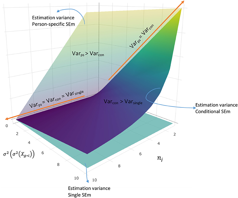
Figure 2. Relationship between the estimation variance of the person-specific -, conditional,- and single error variance, for a fictional examinee i.

Bias

Turning to the (un)biasedness, the following rule holds:

$\begin{array}{l}Rule2.bia{s}_{single},bia{s}_{conditional}\ge bia{s}_{person-specific}\end{array}$

The rationale for this rule is as follows. Using Equations 11 and 12, it is easy to show that the expected value of the estimator $\widehat{{\sigma }^2(E_{{}^{*}i})}$ equals ${\sigma }^2(E_{{}^{*}i})$:

$\begin{array}{rc}{\text{E}}_i\widehat{\left[{\sigma }^2(E_{{}^{*}i})\right]}=K{\text{E}}_i\left[{\sigma }^2(X_{g^{*}i})\right]=K{\text{E}}_i\left[{\sigma }^2(X_{{}^{*}ki})\right]={\sigma }^2(E_{{}^{*}i}).& (23)\end{array}$

Thus, in the long run the error variance of examinee i is correctly estimated. Other estimators are either as unbiased as $\widehat{{\sigma }^2(E_{{}^{*}i})}$ or more biased. Using Equation 8, we see that the expected value of the estimator $\widehat{{\sigma }^2(E_{g^{*}})}$ equals ${\sigma }^2(E_{g^{*}})$. As Equation 9 shows, $\widehat{{\sigma }^2(E_{g^{*}})}$ is only an unbiased estimator for ${\sigma }^2(E_{{}^{*}i})$ when the ${\sigma }^2(E_{{}^{*}i})$ of examinee i equals $\text{E}\left[{\sigma }^2(E_{{}^{*}i})\right]$ over all examinees in ℘. This is either the case when all examinees have the same error variance or when examinee i happens to have an error variance that equals the mean error variance of the population. Finally, based on Equation 16, the expected value of the estimator $\widehat{{{\sigma }^2}_{i\in j}(E_{{}^{*}i})}$ equals ${\sigma }_{i\in j}^2(E_{{}^{*}i})$ when the grouping is based on true scores⁵. $\widehat{{{\sigma }^2}_{i\in j}(E_{{}^{*}i})}$ is thus only an unbiased estimator for ${\sigma }^2(E_{{}^{*}i})$ when the ${\sigma }^2(E_{{}^{*}i})$ of examinee i equals $E_{i\in j}\left[{\sigma }^2(E_{{}^{*}i})\right]$ over all examinees in group j. Again, this occurs when either all examinees in group j have the same error variance or when the error variance of examinee i equals the mean error variance of the group. It is impossible to know whether ${\sigma }^2(E_{{}^{*}i})$ of examinee i happens to be closer to the population mean $\widehat{{\sigma }^2(E_{g^{*}})}$ or the group mean $\widehat{{{\sigma }^2}_{i\in j}(E_{{}^{*}i})}$ and therefore the bias for the single- and conditional SEm are separated by a comma in Rule 2. Figure 3 illustrates Rule 2 graphically (for more detailed information on how Figure 3 was constructed, see the R file “Figure 3.R” on OSF page https://osf.io/6km3z/). The x-axes vary the true error variance of fictional examinee i and the y-axes the variation in true error variances within group j (n_j = 100) where examinee i belongs to. Figure 3A illustrates the bias (estimate of error variance–true error variance) of the single-, conditional-, and person-specific SEm over 10,000 fictional test takes when ${\sigma }^2(E_{{}^{*}i})$ of examinee i equals the group mean $E_{i\in j}\left[{\sigma }^2(E_{{}^{*}i})\right]$, Figure 3B the bias when ${\sigma }^2(E_{{}^{*}i})$ is one standard deviation removed from $E_{i\in j}\left[{\sigma }^2(E_{{}^{*}i})\right]$ and Figure 3C the bias when ${\sigma }^2(E_{{}^{*}i})$ is two standard deviations removed from $E_{i\in j}\left[{\sigma }^2(E_{{}^{*}i})\right]$. The (almost) flat surface for the person-specific SEm in all three plots illustrates that the person-specific SEm is unbiased regardless of the true error variance and variation of true error variances in group j. The tilted vertical surface for the single SEm shows that this SEm is only unbiased when ${\sigma }^2(E_{{}^{*}i})$ collides with the $\widehat{{\sigma }^2(E_{g^{*}})}$. As the first plot shows, when ${\sigma }^2(E_{{}^{*}i})$ equals $E_{i\in j}\left[{\sigma }^2(E_{{}^{*}i})\right]$, both the conditional and person-specific SEm are unbiased (although the surface of the conditional SEm is “bumpier” due to the introduction of variation over the 100 group members). When that is not the case (second and third plot), bias quickly rises when the variance in personal error variances within group j increases.

FIGURE 3

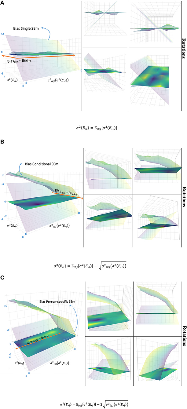
Figure 3. Relationship between the bias of the person-specific -, conditional-, and single SEm variance, for a fictional examinee i. When the error variance of examinee i equals the average error variance in group j (A), both the person-specific SEm and the conditional SEm provide an unbiased estimate. When this is not the case (B,C), the bias of the conditional SEm increases rapidly, with increasing variance over the error variances within group j (y-axis). The single SEm (tilted vertical surface) is only unbiased when the error variance of the examinee (x-axis) coincides with the average population error variance (visible in A–C). To aid interpretation, different rotations of the A–C figure are included at the right side.

Although Rules 1 and 2 and Figures 2, 3 provide insight into the estimation variance and (un)biasedness of the three estimators, it is hard to choose one of the three looking at these two figures separately. Ideally, we would want to choose between the person-specific-, conditional–and single SEm based on the (un)biasedness and variance simultaneously. A measure which naturally fits the need to balance bias and estimation variance is the mean squared error (MSE), which can be expressed as the sum of the bias squared and the estimation variance. In the next sections, we show how to use the MSE to choose between the single, conditional and person-specific SEm in different testing situations.

Simulation

Simulation Design

To compare the single, conditional and person-specific SEm, we simulated item and test scores for 1,000 examinees and 10,000 repeated test takes (see the annotated R file on the OSF page https://osf.io/6km3z/). Six characteristics of the test and the norm population were varied: (1) whether the parallel test scores are continuous and unrestricted or rounded to integers and truncated, (2) the number of repeated test takes, (3) the number of items of the test, (4) the number of parallel test parts K, (5) the relationship between the 1,000 “true” examinee scores and their error variances and (6) the overall reliability of the test. Figure 4 summarizes these six characteristics. Each of these characteristics is also briefly discussed below.

FIGURE 4

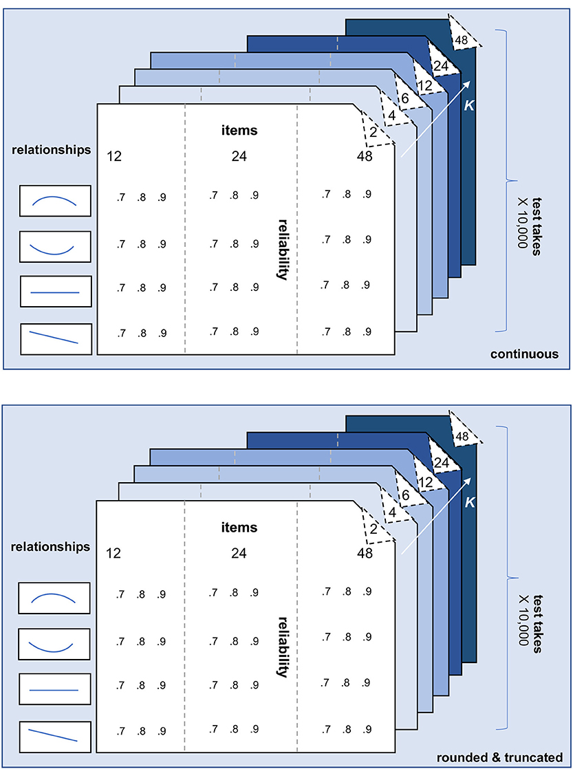
Figure 4. Schematic overview of the simulation design. The characteristics number of repeated test takes (2), number of items (3), number of parallel test parts K (4), relationship between “true” test score and error variance (5), and overall test reliability (6) are varied for both the scenario with continuous test scores (1; upper part of the figure) and rounded and truncated test scores (lower part of the figure). Each slide within “continuous” and “rounded and truncated” belongs to a specific number of parallel test parts K. Within each slide ≤ K = 12, 3 (number of items) × 4 (relationships) × 3 (reliabilities) = 36 conditions are being simulated. The slides K = 24 and K = 48 add another 24 (K = 24) and 12 (K = 48) conditions.

(1) Continuous vs. rounded and truncated scores. As can be seen in Figure 4, all of the other five characteristics are varied for a scenario with continuous item-, parallel-, and total scores and a scenario with rounded and truncated scores. In the “rounded and truncated” scenario (see lower part Figure 4), each item can be answered correctly (item score = 1) or incorrectly (item score = 0), leading to a total score with a possible range between 0 (every item answered incorrectly) and the maximum number of items considered (every item answered correctly). In the “continuous” scenario (see upper part Figure 4), the item- and total scores are on a similar scale as the “rounded and truncated” ones, but these scores are not restricted or rounded. Note that the Classical Test Theory and the formulas for the person-specific SEm, the conditional SEm and the single SEm discussed previously are all based on this continuous scenario. The “rounded and truncated” scenario, however, provides a more realistic reflection of test practice.

(2) Number of repeated test takes. In this simulation study, we simulate 10,000 repeated test takes for each of the examinees. This large number makes it possible to estimate the long run bias, estimation variance and MSE. In practice, however, we do not have 10,000 test takes per examinees and therefore we will also look at fewer test takes (e.g., 1, 2, 3, 4, 5, 10, 25, 50, and 500) to see how accurate SEms estimates are in the short run.

(3) Number of items. Respectively 12, 24, and 48 items are used in this simulation study. Based on previous studies (see, for instance, [5]) 12 items can be perceived as a small test, whereas between 24 and 48 items can be seen as a realistic test size. To keep the simulation results comparable over the varying number of items, for the “rounded and truncated” scenario the relative proportion of items correct of the 1,000 examinees for a certain test take were kept equal (i.e., if person i has 6 items correct on a 12-item test at test take j, he has 12 items correct on a 24-item test at the same test take, et cetera). For the “continuous” scenario, the average item score was kept the same for the varying number of items.

(4) Number of parallel test parts. To compare the effectiveness of various partitions, the 12, 24, and 48 items were respectively divided in parallel parts of K = 2, K = 4, K = 6, and K = 12. For the tests with items > 12, we additionally added K = 24 (24- and 48-item test) and K = 48 (48-item test). By keeping K fixed over the different number of items, the number of items per parallel test part varies. For K = 2, for instance, there are respectively 6, 12, and 24 items in each of the 2 parallel test parts, depending on the number of items in the test. The simulation of the parallel test parts is based on the premise that division of the test in parallel test parts is possible (something that should be checked by the test maker or user in a realistic test situation). On the item level, we thus implicitly assume that the mean item difficulty of the items in every parallel test part is the same. Note that this assumption is harder to fulfill when there are few items in a parallel test part.

(5) Relationship true score and error variance. The choice for either the single-, conditional-, or person-specific SEm also depends on the anticipated relationship between examinees' true scores and their error variance. Users of the conditional SEm, for instance, assume that there is a relationship between true score and error variance whereas such an assumption is not (necessarily) considered when opting for the single SEm or the person-specific SEm. In this simulation study we investigate the influence of four different relationships between true score and error variance, which are all depicted in Figure 5.

The relationships in Figure 5 are all based on the “continuous” scenario. Thus, these relationships show what error variances we might expect for different true scores if there were no test restrictions (i.e., no minimum or maximum scores and no rounding). It is important to stress that the error variances (y-axis) in the “continuous” scenario might differ somewhat from the error variances when test restrictions such as truncation and rounding are taken into account. Due to rounding and truncation, examinees at the extremes, for instance, might have a lower error variance over test takes than in the scenario with continuous scores. On the scale of the test, the results of these examinees are thus relatively consistent and even though the test might make an error theoretically (i.e., the “true” score of an examinee is−15 while he/she keeps getting the minimum score 0 at the test), the test makes this error consistently over test takes, lowering the error variance σ²(E*_i) over test takes. In the results section, the continuous “true” error variances (Figure 5) are used to assess bias and the MSE in the “continuous” scenario whereas the bias and MSE in the “rounded and truncated” scenario are assessed with error variances that are adjusted to take this rounding and truncation into account.

(6) Overall reliability of the test. To test the influence of (overall) reliability, we created data for an overall reliability of 0.7, 0.8, and 0.9. According to often used rules-of-thumb, 0.7 is the minimum acceptable level of reliability, 0.8 is preferred and 0.9 is desirable for high stakes assessment (see [30]). As discussed previously, the reliability of a test for a certain norm population can be expressed as: $\frac{{\sigma }^2(T_{{}^{*}})}{{\sigma }^2(X_{g^{*}})}$; the ratio of the “true” score variance to the total variance in X_g* where ${\sigma }^2\left(X_{g^{\ast }}\right)={\sigma }^2\left(T\ast \right)+{\sigma }^2\left(E_{g^{\ast }}\right)$ (see Equation 7). In our simulation study, we simulate “true” scores for the 1,000 examinees once for all scenario's (see “Simulated dataset(s)” and the x-axis in Figure 5). Therefore, the variance term ${\sigma }^2(T_{{}^{*}})$ in the divisor of the ratio is a constant. To increase the reliability, we manipulated the overall variance (denominator) by lowering the error variance σ²(E_g*). Since ${\sigma }^2\left(E_{g^{\ast }}\right)=E_{}[{\sigma }^2\left(E{\ast }_i\right)]$ (see Equation 9), we divided every of the 1,000 simulated error variances σ²(E*_i) by a certain number d to reach the required reliability level. Note that this division results in a higher overall reliability but does not alter the relationship between true scores and error variances as depicted in Figure 5 (see section above).

FIGURE 5

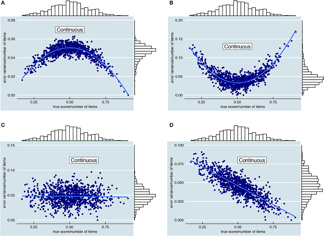
Figure 5. Visualization of the four simulated relationships between “true” total test score (x-axis) and error variance (y-axis). Each dot represents one of the 1,000 fictional examinees. To ease comparison, the error variance and the true score are divided by the number of items in the plots. Note that the y-axis scale depends on the chosen level of reliability. (A) Quadratic relationship between true score and error variance, with lower error variances for examinees with extreme true scores. (B) Quadratic relationship between true score and error variance, with higher error variances for examinees with extreme true scores. (C) Absence of a relationship between true score and error variance. (D) Linearly decreasing relationship between true score and error variance.

Simulated Dataset(s)

True Scores τ_i

Following the simulation design described above, data was simulated in a top-down way, starting with the simulation of the distribution of true test scores τ_i over all 1,000 examinees in ℘. To accommodate different number of items (see Figure 4) we simulated true scores using a standardized metric⁶ and consequently transformed these scores to the scales of 12, 24, and 48 items. Note that the distribution of true scores is fixed over all other scenarios depicted in Figure 4.

Error Variances ${\sigma }^2(E_{{}^{*}i})$

Next, the error variances σ² (E∗_i) were simulated. Just as with the true scores τ_i, the error variances were rescaled for the different number of items. Other than in the case of the true scores, however, the error variances were not fixed over all other scenarios in Figure 4. Rather, the error variance of all examinees varied depending on the anticipated relationship between true score and error variance (see Figure 5) and the overall reliability of the test (which simply shifts the values in Figure 5 down by a factor d). In total, four (relationships true score-error variance) × three (reliabilities) = 12 error variances ${\sigma }^2(E_{{}^{*}i})$were thus simulated for each of the 1,000 examinees.

Total-, Item-, and Parallel Test Scores

For each of the 1,000 examinees and their 12 error variances ${\sigma }^2(E_{{}^{*}i})$ (see above), a vector of 10,000 error scores $E_{{}^{*}i}$ was simulated. Since the three types of SEm are all estimated on the level of parallel test scores, we simulated these error scores on the level of the parallel test parts, $E_{{}^{*}ik}$, first. For this, we made use of the fact that σ²(E*_i) is a sum over the parallel test error variances: $E{\ast }_{ik}~N\left(0,{\sigma }^2\left(E{\ast }_i\right)/K\right)$. $E_{{}^{*}i}$ simply resulted from adding the parallel errors for a certain test take g. To create parallel test scores for each of the 10,000 test takes, the parallel error score was added to the examinee's “true” parallel test score τ_i/K (scaled to the number of items in the test). For the “rounded and truncated” scenario, these parallel test scores were rounded to the nearest integer. When the combination of true score and error resulted in a rounded parallel test score lower than 0 or higher than the number of items/K, the parallel test score was truncated to be zero or equal to the number of items/K, respectively.

Estimation of the SEms, Their Bias and Estimation Variance

After creating the data (see above), the single SEm, conditional SEm and the person-specific SEm were estimated for each of the 1,000 examinees and each of the 10,000 test takes. This process was repeated for all conditions and the “continuous” and “rounded and truncated” scenario separately (see Figure 4). The person-specific SEm was estimated using Equation 11. We subsequently calculated the conditional SEm with Equation 16, using the total score as grouping factor. Since literature on the conditional SEm (see for instance [5]) mentions the additional possibility of grouping examinees in narrow intervals of total scores, we also used Equation 16 for groupings including examinees with different—but adjacent—total scores. Specifically, we used groupings in which the total score ± 1 was used as grouping factor (in the remainder denoted by “con. +1”), total score ± 2 (“con. +2”) and total score ± 3 (“con. +3”). When it was impossible to add or subtract a number from the examinee's total score without crossing the threshold 0 or the maximum score, the largest number was taken which could still be added and subtracted. Thus, “con. +2” means that grouping of examinees is based on total score ± 2 for all total scores ≥ 2 and ≤ the maximum number of items-2, total score ± 1 for total scores 1 and the maximum number of items-1 and just the total score for scores 0 and the maximum number of items, for instance. The single SEm was estimated last based on the Spearman-Brown prophecy formula (see [15]) between the parallel test parts over all examinees within every repeated measurement; ${\rho }_{X{X}^{\prime }}$(see Equation 8). Note that this estimation of the single SEm was based on K = 2, whereas the estimation of the person-specific and the conditional SEms was based on varying K. Finally, the bias squared (${\left[\widehat{{\sigma }^2(E_{{}^{*}i})}-{\sigma }^2(E_{{}^{*}i})\right]}^2$) was estimated for all 1,000 examinees and all conditions ($\widehat{{\sigma }^2(E_{{}^{*}i})}$ is the average estimate of ${\sigma }^2(E_{{}^{*}i})$ over the 10,000 test takes). This bias squared was added to the estimation variance (${\sigma }^2(\widehat{{\sigma }^2(E_{{}^{*}i})})$) over the 10,000 test takes to calculate the MSE.

Results

In the simulation design, six characteristics of the test and the norm population were varied: (1) whether the parallel test scores are continuous and unrestricted or rounded to integers and truncated, (2) the number of repeated test takes, (3) the number of items of the test, (4) the number of parallel test parts K, (5) the relationship between the 1,000 “true” examinee scores and their error variances and (6) the overall reliability of the test. Below, the influences of each of these characteristics on the bias, estimation variance and MSE of the three kinds of SEm are discussed.

Continuous vs. Rounded and Truncated

When parallel test scores were rounded and truncated, we saw an alteration of the simulation results. This alteration had two general causes: (1) the error variances as depicted in Figure 5 were altered and (2) rounding and truncation limited the between variance over parallel test parts. Each of these two causes is discussed below. Because of the influence of rounding and truncation, in the other sections results are discussed separately for the “continuous” and the “rounded and truncated” case.

Alteration of the Error Variances

The error variances ${\sigma }^2(E_{{}^{*}i})$ as displayed in Figure 5 are based on continuous parallel test scores. Rounding and truncating these parallel test scores alters the total test scores—the sum over the parallel test scores—and thus the error variances. In a sense, rounding and truncation thus “push” the error variances in a certain direction that takes into account the limitations of the scale of the test. In Figure 6, an example of the possible extreme influence of rounding and truncation on the error variances ${\sigma }^2(E_{{}^{*}i})$ is showed. This example is based on the relationship in Figure 5A and 12 items; comparable plots for the other relationships of Figure 5 and 24 and 48 items can be found in the Supplementary Material, Part I.

FIGURE 6

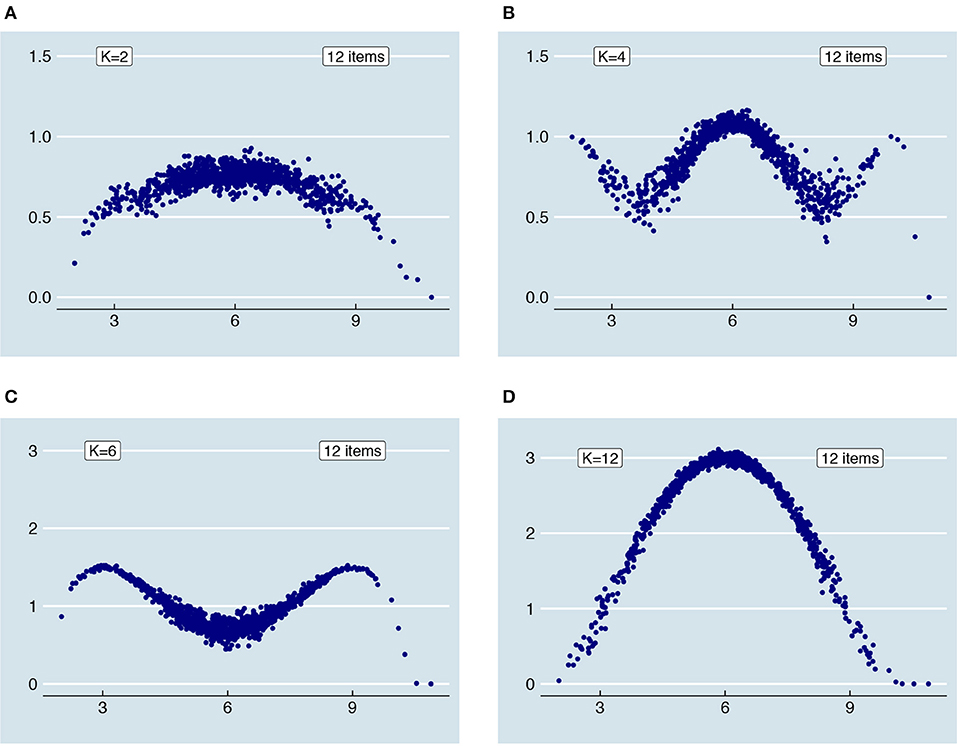
Figure 6. Influence of rounding and truncation on error variances for a test with 12 items, a .8 reliability and K = 2, 4, 6, and 12 respectively. Note the difference in scale of (A) and (B) vs. (C) and (D).

Based on Figure 6 and Supplementary Material, Part I, a few observations can be made. First, since rounding and truncation take place on the level of parallel test scores, the choice for K influences the error variances. Figures 7, 8 illustrate why this is the case. These two figures are based on two example examinees for a test with 12 items and K = 4. The first examinee has a “true” test score of 4; the second a “true” test score of 6. Before rounding and truncation, these two examinees have the exact same error variance of 0.20; after that an error variance of respectively 0.10 and 1.00. Looking at the distribution of parallel test scores (Figure 7) for the examinee with true score 4 (Figure 7A) and the examinee with true score 6 (Figure 7B) we see that there is indeed very little variation in the parallel test scores for the first examinee while there is a relatively large variation in the second examinee's case, due to an (almost) equal amount of parallel scores 1 and 2. Looking at the underlying continuous error distributions for one of the parallel test parts (Figure 8), we see that there is (almost) no difference between the two examinees. What is different is the effect of the error on the rounded parallel test score. Since the score 4 is divisible by K = 4, the continuous “true” parallel test score is 1. Only when the parallel test error is larger or equal to 0.5 or smaller or equal to −0.5, the parallel test score will be rounded one score up and down, respectively. Since the score 6 is not divisible by K = 4, the continuous “true” parallel test score is 1.5. Any negative error larger than −0.000⋯1 leads to a rounding down to 1 whereas any positive error smaller than 0.999⋯9 has no influence on the rounded score. Thus, although the original errors of examinee 1 and 2 are similar due to their similar (continuous) error variance, the effect of these errors on the rounded parallel test scores is different. Would we change K to another number, say 3, then the effect of the error on the rounded parallel test score would change accordingly.

FIGURE 7

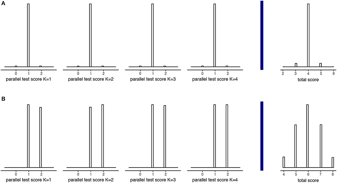
Figure 7. Parallel and total test scores for two example examinees with true score 4 (A) and true score 6 (B), both having a true error variance of 0.2 on a 12 item test with K = 4.

FIGURE 8

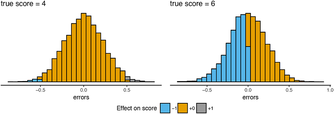
Figure 8. Error score distribution for the first parallel test and the effect on the parallel test score for the two examinees of Figure 7.

A second observation is that the truncated and rounded error variances reassemble the continuous error variances more closely when the number of items is larger (see Supplementary Material, Part I). Generally, when there are more than 3 items within each parallel test part, the distribution of truncated and rounded error variances is very similar to that of the continuous one. Last, in the extreme case of having only one item within each parallel test part, the relationship between “true” score and error variance becomes more or less parabolic regardless of the “original” relationship as depicted in Figure 5. In that case, the error variances approximate those of a binomial distribution (see [23]); they become a compromise between the simulated relationship and a binomial one. In Figure 9, the relationship between “true” scores and error variances is shown for 12 items and K = 12 together with the binomial error for comparison.

FIGURE 9

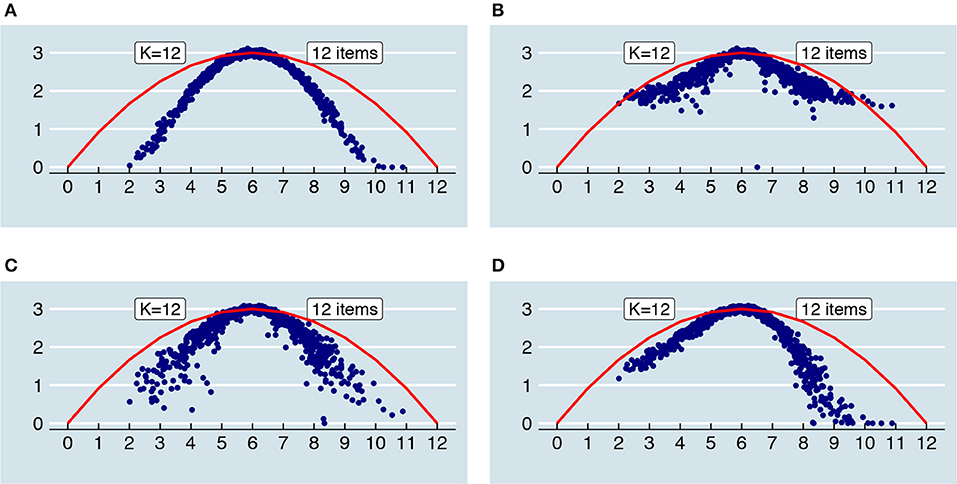
Figure 9. When the parallel test scores are truncated and rounded, the relationships between “true” scores and error variances as depicted in Figure 5 change. In the extreme case, when there are only 12 items and K = 12, the relationship between “true” scores and error variances of an originally quadratic increase (A), quadratic decrease (B), flat relationship (C) and linear decrease (D) all more or less reassemble that of the red parabola, which corresponds to the binomial error of a 12-item, dichotomously scored test.

In the section “Bias-Variance Trade-Off,” it was explained that the person-specific SEm provides an unbiased estimate of ${\sigma }^2(E_{{}^{*}i}).$ As visualized in Figure 10, this holds when parallel test scores are continuous (Figure 10A) and when parallel test scores are rounded and truncated (Figure 10B). Equation 11 thus holds when we use it based on continuous parallel test scores to estimate the continuous ${\sigma }^2(E_{{}^{*}i})$ as depicted in Figure 5. Likewise, when we use the person-specific SEm based on rounded and truncated parallel test scores we obtain an unbiased estimate of the rounded and truncated ${\sigma }^2(E_{{}^{*}i})$counterpart (see Supplementary Material, Part I). The person-specific SEm based on rounded and truncated parallel scores only gives an unbiased estimate of the continuous ${\sigma }^2(E_{{}^{*}i})$in so far as the continuous and rounded and truncated ${\sigma }^2(E_{{}^{*}i})$are similar.

FIGURE 10

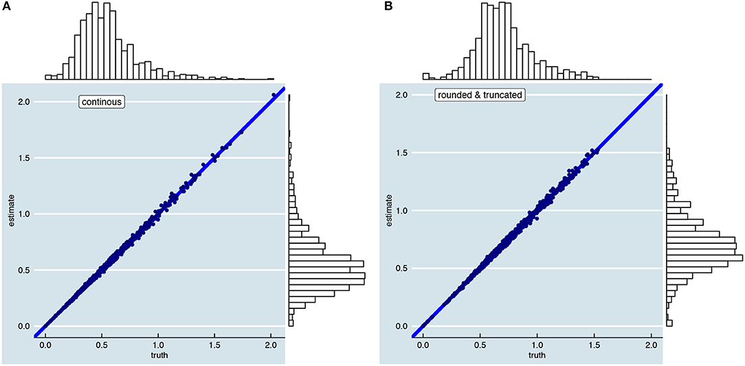
Figure 10. Visualization of unbiasedness of the person-specific SEm over 10,000 repeated test takes. The left figure (A) is based on continuous parallel test scores; the right figure (B) on rounded and truncated test scores. The two figures are examples of a test with 12-items, K = 2, a reliability of 0.8 and a relationship between “true” score and error variance as shown in Figure 5B.

Limits on Between Variance

When the number of items in a parallel test part is small and/or the size of K is small, truncation and rounding lead to another problem: the number of possible between variances becomes limited. Since the person-specific and the conditional SEm are based on the between variance over parallel test parts, this also means that the possible estimates for ${\sigma }^2(E_{{}^{*}i})$ are limited. With 12 items and K = 12, for instance, only 13 unique combinations can be made of 0 and 1 scores (note that Equation 24 is an adjustment of the formula for combinations with replacement):

$\begin{array}{rc}\frac{(n_s+K-1)!}{K!(n_s-1)!}=\frac{(2+12-1)!}{12!(2-1)!}=13& (24)\end{array}$

where n_s denotes the number of possible scores (in this case, 2; 0 and 1). With these 13 combinations, only 7 unique between variances can be obtained. Thus, using Equation 11, there are only 7 possible estimates of the person-specific SEm at every test take. When there are such few options, there is a high chance that none of the possible SEm estimates are close to the true ${\sigma }^2(E_{{}^{*}i})$ of the examinee. In the long run this is not problematic, since we average over the ${\sigma }^2(E_{{}^{*}i})$-estimates and thus are still able to obtain an unbiased overall estimate. But when we only have one test take (as we usually do) this is troublesome.

Figure 11 shows the options for the between variance when there are respectively 12 items with K = 2, 4, 6, and 12. In the Supplementary Material, Part II, the same figure is available but then for tests with respectively 24 and 48 items. Looking at Figure 11, there are the fewest options for the ${\sigma }^2(E_{{}^{*}i})$-estimate when either the size K is small (i.e., K = 2) or when there are few items within each K (i.e., K = 12). An important distinction between having a small K vs. having few items within each K is, however, that most of the options are within the range of the actual error variances with K = 12 whereas most of these options are outside this range when K = 2. A reasonable number of items (see Supplementary Material, Part II) and a balance between not having too few parallel test parts but also not too few items within each K seems essential.

FIGURE 11

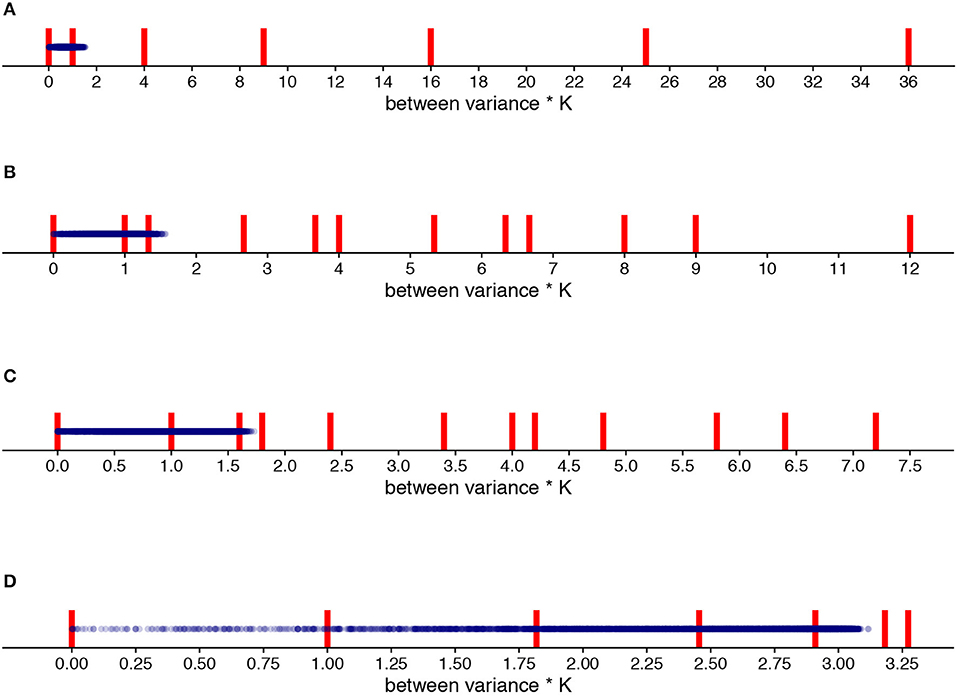
Figure 11. All options of the between variance multiplied by K (red vertical lines; see Equation 11) for K = 2 (A), K = 4 (B), K = 6 (C) and K = 12 (D) compared to the “true” truncated and rounded error variances of the 1,000 examinees (blue dots). Note the difference in x-axis scale.

The conditional SEm also suffers from having few estimation options when K and the number of items within K are small. However, since the conditional SEm consists of taking an average over similar examinees, the number of estimation options accumulates the more examinees are taken together. With only one extra examinee, for instance, there are 7² possible combinations of between variances for the example of 12 items and K = 12 of which 27 lead to a unique between variance estimate when averaged. This more than doubling notwithstanding, in practice the problem of having few options can still occur. Especially when there is a notable relationship between “true” score and error variance, it is likely that we average over just one or a few between variance options.

Number of Repeated Test Takes

In the section “Bias-Variance Trade-Off” we discussed the long run properties of the three different SEm estimators. However, favorable long run properties do not guarantee that the SEm estimator is appropriate to use in the short run, when only having one or just a few test takes. Below, we discuss the short run properties of the person-specific and the conditional SEm (not the single SEm, since this SEm does not change with more or less test takes) and reasons why the person-specific and conditional SEm might not be as appropriate to use in the short run as in the long run.

Short Run Performance of SEm

To see how well the conditional and person-specific SEm perform in the short run, we plotted these SEm estimates after only 1, 2, 3, 4, 5, 10, 25, and 50 test takes, together with the true error variances we are trying to estimate⁷, for both the scenario with continuous parallel test scores and rounded and truncated parallel test scores. The result can be seen in the Supplementary Material, Part V. The Pearson correlation between the true error variance and the estimates are shown at the right side of the plots. Additionally, a table is presented with the within variance at true error variance 0.6 and the between variance over all examinees. When there is only one test take, the correlation between the truth and the SEm estimates is very low for the person-specific SEm (only 0.09 in both the continuous and rounded and truncated case). The conditional SEm is only slightly better (0.20 in the continuous case and 0.12 in the rounded and truncated case). The SEm estimates for different true error variances appear to overlap to a large extent, although variation in the SEm estimate increases along the x-axis and higher estimates are observed occasionally for higher true error variances. After 50 test takes, the correlation has increased notably but the variance in estimated SEm for examinees with 0.6 as their “true” error variance is still about the same as the overall between variance. As Figure 12 shows, about 100 (conditional SEm, Figure 12B) to 200 (person-specific SEm, Figure 12A) test takes are needed to reach high levels of correlation. When parallel test scores are rounded and truncated (second part Supplementary Material, Part V), we generally need more test takes (see Supplementary Material, Part VI, which contains the equivalent to Figure 12 for rounded and truncated parallel test scores). The correlations are therefore generally lower than in the continuous case.

FIGURE 12

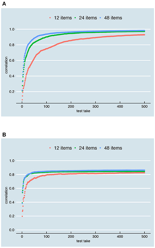
Figure 12. Correlation between the true error variance and the SEm-estimate for different number of test takes (x-axis) and a test with respectively 12, 24, and 48 items. (A) Shows the correlations for the person-specific SEm; (B) A comparable figure for the conditional SEm. Both are based on continuous parallel test scores, an overall reliability of 0.8 and a relationship between “true” score and error variance as depicted in Figure 5A.

Reasons for Bad Short Run Performance

We found two general reasons for the suboptimal short run performance as observed in Supplementary Material, Part V and Figure 12. One of these reasons was already discussed in the previous section and visualized in Figure 11: because of few possible between variances, the SEm for a single test can only take on few different values. This influence is clearly visible in the first plot of the “rounded and truncated” scenario in Supplementary Material, Part V. There is also another reason why the person-specific (and to a certain degree the conditional SEm) might not be suitable estimators of the error variance after one or just a few test takes, even when parallel test scores are continuous. As visualized in Figure 13, the distribution of possible between variances for different underlying error variances overlap to a high extent, especially in the small between variances range. Therefore, if we would randomly observe one between variance it can be the result of very different underlying error variances. As Figure 13 shows, a problematic feature of the distributions of between variances is that the variance of this distribution directly depends on the size of the underlying error variance (see Equations 19 and 20 and the sd in Figure 13).

FIGURE 13

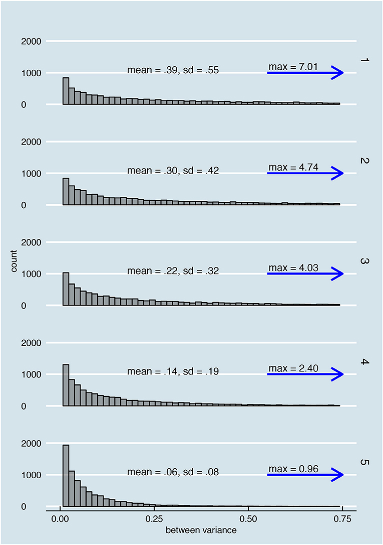
Figure 13. Overlap in the distributions of possible between variances for 5 examinees with underlying error variances 0.75 (examinee 1), 0.60 (examinee 2), 0.44 (examinee 3), 0.28 (examinee 4), and 0.12 (examinee 5).

Therefore, the accuracy of any estimate based on the between variances directly depends on that what we are trying to estimate; the error variance. Since the error variance is unknown, we do not know exactly how accurate we can expect one estimate to be. Other problematic features of the distribution of between variances are that zero is always the most probable between variance, no matter how large the underlying error variance (see again Figure 13 and the overabundance of zeroes in Supplementary Material, Part V) and that the distribution has a large tail. Regarding the former, we might be tempted to conclude that there is little error variation when we observe a between variance of zero but the underlying error variance might actually be relatively large. With regard to the latter, for comparison purposes Figure 13 only shows the histogram values until 0.75, but as the blue arrow and the “max = .” shows, the distributions are stretched out over a far wider range. The large between variances are rare, but they are necessary to reach an accurate estimate on average. Due to the relationship between error variance and variation in the possible between variances, observing a low between variance does not contain as much information about the underlying error variance as does observing a high between variance. Whereas a low between variance can be the result of small, medium or even large error variances, a large between variance is very unlikely to be the result of a small or even medium error variance. Finally, the distribution of between variances does not become less spread out when we include more items or increase K.

Number of Items

By incrementing the number of items, the scale of the parallel test scores and hence the size of the true error variances (see Figure 5, Supplementary Material, Part I) increased. Consequently, comparing the absolute bias, estimation variance and MSE is not very insightful, as it simply reflects this change in scale. To compare the bias and estimation variance for the different number of items, we therefore decided to use a relative version. Specifically, we express bias as a percentage of the true error variances:

$\begin{array}{cc}\%\text{bias}=\left[\frac{{\displaystyle {\sum }_i\left(\widehat{{\sigma }^2\left(E{\ast }_i\right)}-{\sigma }^2\left(E{\ast }_i\right)\right)}}{{\displaystyle {\sum }_i{\sigma }^2\left(E{\ast }_i\right)}}\right]100& (25)\end{array}$

and we use the coefficient of variation (see [24]) as a relative measure of estimation variance, which is simply the estimation standard deviation expressed as a percentage of the mean:

$\begin{array}{rc}\text{CV}=\left[\frac{{\displaystyle {\sum }_i}\sqrt{{\sigma }^2({\sigma }^2(E_{{}^{*}i}))}}{{\displaystyle {\sum }_i}{\sigma }^2(E_{{}^{*}i})}\right]100& (26)\end{array}$

Below, we discuss the percentage bias and coefficient of variation when compared over tests with different lengths (i.e., with 12, 24, and 48 items). We also discuss whether and how having a larger test is beneficial for the SEm-estimates.

Percentage Bias

In Figure 14, the percentage bias is visualized for different number of items, for the relationship depicted in Figure 5A and with continuous parallel test scores (for the other relationships, see Supplementary Material, Part IV). According to this figure, bias is not dependent on the number of items in the test (all bars are of equal height for the person-specific, conditional and single SEm). Note that the percentage bias for the person-specific and conditional SEm is very close to zero, but not exactly null. The small deviation from zero stems from the fact that we have a limited norm population size (1,000) and a limited number of repeated test takes (10,000) over which we determine the bias. The covariance between the parallel test parts (see Equation 10a) over the 10,000 test takes are, for instance, very close to zero, but not exactly zero (as Equation 10b assumes). The “$2\sum _{k<p}{\sigma }^2(X_{{}^{*}ki},X_{{}^{*}pi})$” part in Equation 10a for the first five examinees for a test with 12 items, 2 parallel test parts, an overall reliability of 0.8 and a relationship as in Figure 5A, are for instance −0.00056, −0.001686, −0.004748, −0.000355, and −0.014109. Therefore, the between variance (see Equation 12) on which the person-specific and conditional SEm are based is not exactly equal to the within variance of Equation 10a, leading to a small bias over the limited set of test takes. As Equation 12 postulates, this bias is expected to disappear with an infinite number of tests.

FIGURE 14

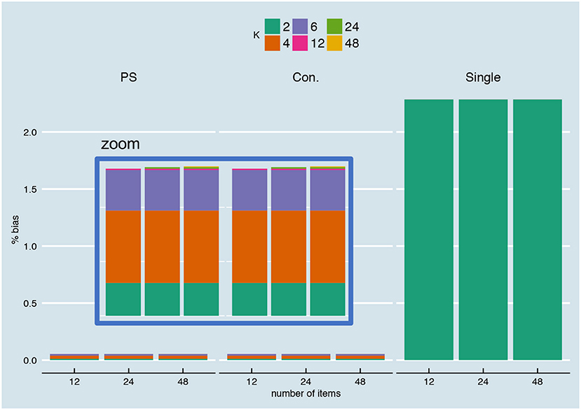
Figure 14. Percentage bias (see Equation 25) for different number of items, for the relationship depicted in Figure 5A and with continuous parallel test scores.

When parallel test scores are rounded and truncated, the percentage bias as observed in the continuous case changes (see Supplementary Material, Part IV). Due to truncation and rounding, the percentage bias is not exactly the same anymore for different test lengths. The percentage bias now depends on the changed relationship between “true” test score and error variance (see Supplementary Material, Part I) and the between variances that can be estimated with a certain number of items and K (see Supplementary Material, Part II). Additionally, the percentage bias decreases in the case of the “con.+1,” “con.+2,” and “con.+3” when moving from a 12-item to respectively a 24-item and 48-item test. This has to do with the fact that “+1” is a larger step in a 12-item test (1/12th) than in a 24-item test (1/24th) or a 48-item test (1/48th). Hence, we introduce relatively more bias when we include examinees with +1 scores when the scale of the test is smaller (and similarly for examinees with +2 and +3 scores).

Coefficient of Variation

Figure 15 shows the coefficient of variation for different number of items for the relationship depicted in Figure 5A with continuous parallel test scores (for the other relationships, again see Supplementary Material, Part IV). Not surprisingly, the coefficient of variation is exactly the same over different numbers of items for the person-specific SEm and the single SEm. As expressed earlier in Equation 19 and Equation 20, the estimation variance of the person-specific SEm does not depend on the number of items. The single SEm has a small random variation from test take to test take (since the scores of the norm population change randomly over test takes), but this random variation also does not depend on the number of items. For the conditional SEm, there is a small increase in the CV when moving from a 12- to a 24- and 48-item test. Inspection of Equation 21 shows that the estimation variance for the conditional SEm not only depends on K (as the variance for the personal SEm) but also on n_j; the number of examinees within one group j. Since we kept the overall number of examinees (1,000) equal over the different test lengths, the number of examinees with the same total score decreased when doubling the number of items from 12 to 24 and from 24 to 48; leading to the slight increase in CV.

FIGURE 15

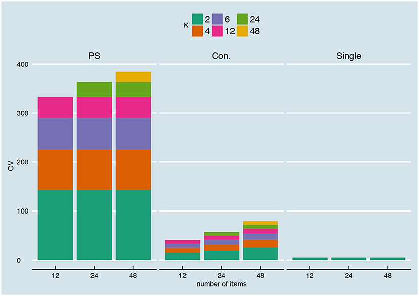
Figure 15. Coefficient of variation (see Equation 26) for different number of items, for the relationship depicted in Figure 5A and with continuous parallel test scores.

When parallel test scores are rounded and truncated, the CV changes (see Supplementary Material, Part IV). For the person-specific SEm, the CV is not exactly the same anymore over the different test sizes. Additionally, the CV becomes smaller when moving from a conditional to a conditional “+1,” “+2,” and “+3” for a fixed test size. This again has to do with the n_j in Equation 21. Because of the +1, +2, and +3, more examinees are included in a group j leading to a smaller estimation variance. This decrease in CV is largest for the 12-item test since—as discussed previously—the +1, +2 and +3 are relatively larger intervals in a smaller test. Including examinees with +1 therefore increases n_j faster for a smaller test.

Benefits of Having a Larger Test

Looking at Figures 14, 15 and Supplementary Material, Part IV, in the long run there is no advantage in having a larger test when estimating the SEm. The relative bias and estimation variance do not change when increasing the number of items, as bias and estimation variance do not depend on test length (see section “Bias-Variance Trade-Off”). When using rounded and truncated parallel test parts, however, there is an advantage in having a larger test as discussed in the previous sections. With a larger test size, the estimable error variance depends less on K and the between variance can take on more different values. Additionally, in the short run the SEm estimates are more accurate when based on a larger test. As Figure 12 showed, with a larger test, initial correlations between true error variance and the SEm estimates are higher and there are fewer repeated test takes needed to reach a high correlation.

Number of Parallel Test Parts

Figure 15 (previous section) shows why it is beneficial for the person-specific and conditional SEm to choose K as high as possible when parallel scores are continuous: the estimation variance goes down with increasing K. This relationship between the estimation variance and K was also discussed in the section “Bias-Variance Trade-Off.” A more puzzling result of the previous section (see Figure 14) is that the relative bias observed after 10,000 test takes also seems to depend on K to some extent. In Figure 14, the relative bias of K = 12 is, for instance, structurally lower than the relative bias of K = 4 (also see Supplementary Material, Part IV). It is unclear why this difference in bias for different values K occurs, especially since it is not linearly related to K. Since we are using a limited number of repeated measures (10,000) and a limited sized norm-population (1,000 examinees) and R has a limited precision in its calculations, the differences observed may be a reflection of these limitations instead of real differences over K. Inspection of the average SEm-estimates with different sizes for K at least shows that the absolute differences are neglectable in any practical situation. All in all, the comment that it is “advantageous to use as many [parallel] parts as possible” ([5] p. 154) seems to hold in the case of continuous parallel test scores.

When parallel test scores are rounded and truncated, the choice for K becomes more delicate. As was already discussed in the section “Continuous versus rounded and truncated,” the observable error variance depends on characteristics of the test, including the size of K. When every parallel part contains few items, the resulting error variance estimate highly depends on K and therefore the estimate of the error variance cannot be generalized to a similar test with larger or smaller K. Furthermore, the choice for K influences the between variances that can be observed (see again Figure 11). Instead of opting for the largest K possible, it therefore seems advisable in case of rounded and truncated scores to balance K and the number of items within each parallel test part.

Relationship True Score and Error Variance

In this simulation, we varied the relationship between “true” score and error variance according to Figure 5. The question is whether the preference for one of the different SEms depends on these underlying relationships. Figure 16 shows a grid with all possible combinations of K, the number of items and the overall reliability for the relationships depicted in Figure 5A (Figure 16A), Figure 5B (Figure 16B), Figure 5C (Figure 16C), and Figure 5D (Figure 16D). The colors within this grid show which of the three SEms had the lowest absolute MSE and thus would be favored in which situation. Figure 17 shows similar figures but for the case with rounded and truncated parallel test parts. In these figures, also the conditional “+1”, “+2,” and “+3” are included.

FIGURE 16

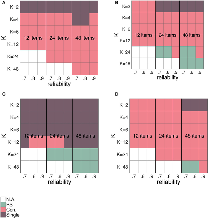
Figure 16. Preference for the person-specific SEm (green), the conditional SEm (pink) or the single SEm (purple) based on the MSE for different K's, number of items and overall reliability. Plot (A) corresponds to the relationship between “true” scores and error variances as depicted in Figure 5A, (B) to the relationship of Figure 5B, (C) to the relationship in Figure 5C and (D) to the relationship in Figure 5D. All four plots are based on continuous parallel test scores.

FIGURE 17

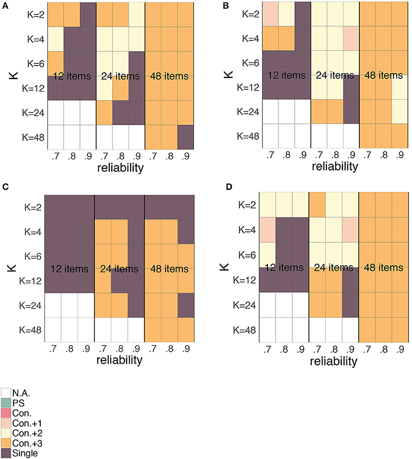
Figure 17. Preference for the person-specific SEm (green), the conditional SEm (pink), the conditional SEm “+1” (light pink), the conditional SEm “+2” (yellow), the conditional SEm “+3” (orange) or the single SEm (purple) based on the MSE for different K's, number of items and overall reliability. Plot (A) corresponds to the relationship between “true” scores and error variances as depicted in Figure 5A, (B) to the relationship of Figure 5B, (C) to the relationship in Figure 5C and (D) to the relationship in Figure 5D. All four plots are based on rounded and truncated parallel test scores.

Turning first to Figure 16, we see a comparable pattern for all relationships exact for the “flat” or “no relationship” case (Figures 5C, 16C). When no relationship between “true” score and error variance is anticipated, the single SEm is generally the best choice unless the number of items and K are large. When we do anticipate a relationship between “true” score and error variance, the conditional SEm is generally favored, unless K is small relative to the number of items (favoring the single SEm) or when both the number of items and K are large (favoring the person-specific SEm).

Looking at Figure 17, we see again some comparability over all relationships except for Figure 17C. For the “flat” or “no relationship” case (Figure 17C), the single SEm is again favored most, together with the conditional SEm with a large interval width. Opposed to the single SEm, the “con.+3” can adjust its estimate such that the error variances for “extreme” true scores are correctly estimated. Since variation at these extremes of the scale (see Figure 5C) is less than in the middle, having a SEm-estimate close to the real error variances at these extremes lowers the overall discrepancy between the estimated SEm and the true error variances. In the other three figures, the “con.+3” option is also a popular choice. To a lesser extent, also the “con.+1” and “con.+2” options are favored over the person-specific and the “regular” conditional SEm. The popularity of the conditional SEms with a larger interval makes sense, because they are stable (like the single SEm) but also flexible enough to capture the anticipated relationship between “true” score and error variance. They also lead to the largest possible group size n_j, which directly lowers the estimation variance (see section “Bias-Variance Trade-Off”). Other than in the case of continuous parallel test scores, the single SEm is not chosen when K is small relative to the number of items. For rounded and truncated scores, the single SEm is for instance favored when the number of items is small (i.e., 12) and K relatively large. In the section on rounding and truncation, we saw that the relationship between true score and error variance was highly altered when the number of items was small relative to K (see Figure 6). For a 12-item test, this influence was already present with a K larger than 2. When such an alteration occurs, it is better to stick with the single SEm (which is always based on K = 2, see section “Simulated Dataset(s)”) than to opt for a conditional SEm with a larger K.

Overall Reliability

As explained under “simulation design,” the overall reliability of the test was manipulated by dividing every examinee's error variance by d. Since this lowers the size and therefore the scale of the error variances, we expect the bias², estimation variance and MSE to go down when moving from a 0.7 to a 0.8 and 0.9 overall reliability. Figure 18 shows that this is indeed the case for a test with 24 items, with K running from 2 to 6 and error variances as in Figure 5A (similar figures for other number of items, K and error variances can be requested from the first author). In this figure, the reliability is varied on the x-axis and every type of SEm is shown separately (note the difference in y-axis for the person-specific SEm compared to the other SEms). Despite the decrease in bias² in absolute sense, there is no clear downward trend in the percentage bias (see Table 1, Equation 25). Additionally, the relative differences in MSE, bias² and estimation variance between the single, person-specific, and conditional SEms are comparable regardless of whether there is an overall reliability of 0.7, 0.8 or 0.9 (see Figure 18). Figure 18 furthermore shows that the proportion of the MSE “caused” by bias is not notably different for the different overall reliability except for the conditional SEm (see percentages on top of the bars in Figure 18). This bias inflation for relatively low reliabilities is caused by using the total score instead of the true score of examinees as grouping factor in the calculation of the conditional SEm (see [22]). The higher the overall reliability, the smaller the difference between the total and true scores and thus the less bias is introduced in the grouping.

TABLE 1

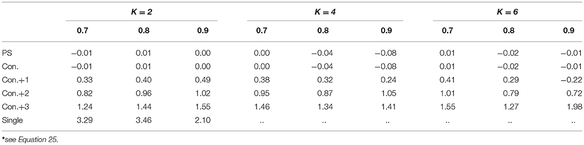
Table 1. Percentage bias* accompanying Figures 18A–C.

FIGURE 18

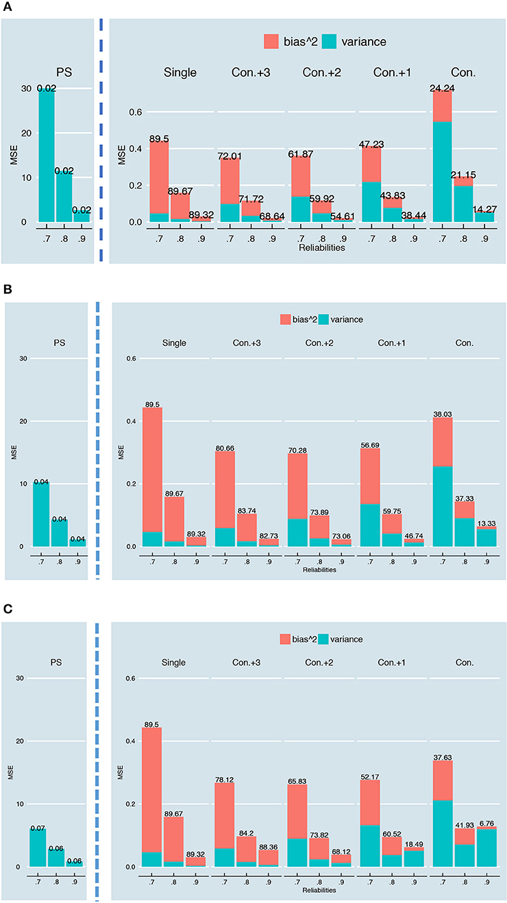
Figure 18. Bias², variance and MSE for a test with 24-items and K = 2 (A), K = 4 (B), and K = 6 (C) parallel test parts. The overall reliability of the test is varied on the x-axis. The numbers on top of the bars show the percentage of the MSE “caused” by the bias², which is also reflected in the size of the stacked pink bar. Note that these plots are based on the relationship in Figure 5A; similar plots for the other relationships can be requested from the first author.

The results shown so far are all based upon rounded and truncated parallel test scores. Supplementary Material, Part III contains similar plots as in Figure 18, but then for continuous parallel test scores. Generally, the results with continuous and rounded and truncated parallel test scores are very similar. The MSE, bias² and estimation variance are, however, overall somewhat lower when no rounding and truncation have taken place. Also, rounding and truncation apparently increase the bias² notably when opting for a conditional SEm; in the continuous case (see Supplementary Material, Part III) the MSE of the conditional SEm is almost completely caused by estimation variance.

Discussion

By convention, the single standard error of measurement (SEm) is used to express measurement (un)certainty of examinees (see Equation 8). By using this single SEm, two strict assumptions are made regarding measurement (un)certainty. First, it is assumed that all persons are measured with the same accuracy; i.e., measurement error variance is assumed constant. Second, the person's intra-individual variation in measurements is assumed equal to the inter-individual variation in measurement of the norm-population examinees; i.e., intra-individual variation and inter-individual variation are interchangeable [6]. To circumvent these assumptions, one can also opt for the conditional SEm. The conditional SEm relaxes the two assumptions in that only examinees with the same (expected) true scores are assumed to have constant measurement error variance and interchangeability of inter- and intra-individual variation. Instead of basing the estimate of SEm on all examinees in the normpopulation, like the single SEm, the conditional SEm takes the expected value of the person-specific measure of SEm over all examinees with the same obtained total score (see Equation 16). In the conditional SEm literature, this person-specific measure of SEm is treated as an intermediate step but—as this paper showed—can also be used as a result on its own. Using this person-specific SEm has the advantage that no assumptions are made regarding measurement (un)certainty (see Equation 11). Every relaxation of the two assumptions of the single SEm—however—comes with a price: in practice, the estimation variance of the conditional SEm and person-specific SEm always exceed the estimation variance of the single SEm⁸. In this paper, we have illustrated how the mean squared error (MSE)—a measure that is based on both estimation variance and bias—can be used to make a choice for either the single, the person-specific or the conditional SEm in realistic test situations. This “optimal” SEm guarantees that the estimated SEm is as close as possible to the true error variance of examinees. We also showed, using a simulation study, how the person-specific SEm, the conditional SEm and the single SEm are influenced by six characteristics of the test situation: (1) whether the parallel test scores are continuous and unrestricted or rounded to integers and truncated, (2) the number of repeated test takes, (3) the number of items of the test, (4) the number of parallel test parts K, (5) the relationship between the 1,000 “true” examinee scores and their error variances and (6) the overall reliability of the test. Refraining from repeating all findings for each of these six characteristics here, we like to highlight three important overall conclusions from the simulation study. First, it is important to realize that the three different SEms are developed for a situation with continuous test scores. When scores are rounded and truncated—as they typically are in practice—we face a number of challenges in the estimation of the person-specific and the conditional SEm that we should keep in mind. Second, it is important to stress that even though the MSE helps to balance long run unbiasedness and estimation variance, it does not guarantee that the estimates for a single test take make sense. Rounding and truncation can for instance lead to sparseness in the possible SEm-estimates (see Figure 11), such that no single estimate can be close to the real error variance after one test take. One single estimate also relatively often equals zero, since zero is the between variance that most often occurs for any underlying error variance (see Supplementary Material, Part V). It would be dangerous to conclude that this examinee is thus measured very accurately, since the underlying error variance can still be large. Third, it is advisable to think about the purpose of the SEm-estimation, and to choose accordingly. The conditional SEm, for instance, can be suitable in certain test situations to get an idea of how variable we expect the test scores to be. It might not be so suitable, however, to construct a confidence interval and to see whether this confidence interval overlaps with or is smaller/larger than the confidence interval of another examinee. Since both the total score and the SEm on which the confidence intervals are based vary, we don't want to draw conclusions that might be based on random error in one or all total scores and one or all error variances. It might be fairer to use the single SEm in that case. As a last example: the person-specific SEm might not be suitable in a certain situation as a direct measure of error variance but it could be suitable to select examinees for which the estimate is relatively large. Since large between variances are rare (or non-existent) for small and medium error variances (see Figure 13), a large between variance points to a large underlying error variance. This can be a reason to be careful with using the single SEm for this specific examinee. In order to help making a choice between the single, conditional and person-specific SEm, we end with a set of practical recommendations.

Practical Recommendations

This paper shows that there is not one type of SEm (i.e., single, conditional with different sizes of intervals or person-specific) that is superior in every test situation. Therefore, in order to choose one must first come to a realistic estimation of the “truth” (i.e., how strong is the anticipated relationship between true score and error variance? How “unique” do we expect the error variances of different examinees to be?) and a realistic idea of the limits and possibilities of the test (i.e., how reliable is the test for the examinees that you have/had in mind? How many parallel or tau-equivalent parts K are feasible, taking for instance the item difficulties and item content into account?). Preferably, this endeavor is followed by a small simulation to find the optimal balance between bias and variance in the error variance estimate(s). Alternatively, one could use the following rules of thumb, based on the results of our simulation:

• When a test is based on a limited set of items and/or can only be divided in a limited set of parallel (or tau-equivalent) test parts K, the gain in (less) bias does not make up for the loss (increase in) estimation variance. In such a situation, either use the single SEm or a conditional SEm in which you make coarse intervals. When you do not expect a relationship between “true” score and error variance (Figure 5C), selecting the single SEm is most appropriate in this situation.

• When the overall reliability of the test for a group of examinees is low, be cautious in the interpretation of the conditional SEm. The single SEm is preferred in this case, except when you expect a strong relationship between true score and true error variance.

• Opting for a person-specific SEm is only encouraged when you either have continuous parallel test scores plus a large number of items and a large K (see Figure 16) or when it is possible to test an examinee multiple times (see [20]).

• Be sure to have at least three items in every parallel test part if your test consists of rounded and truncated scores, to minimize the influence of truncation and rounding. Where possible, check the limitations that rounding and truncation put on the possible between variances (see Figure 11) and see whether taking an average over similar examinees (conditional SEm) solves these limitations.

• When in doubt, choose a conditional SEm with coarse intervals (i.e., “con.+3”). Especially when you anticipate a relationship between “true” score and error variance, the conditional SEm with coarse intervals is able to capture the main trend whilst being a fairly stable estimate.

Author Contributions

KL and RV both contributed to the study idea and design. KL conducted the simulation and wrote and revised the paper with feedback of RV.

Funding

KL is supported by a NWO-talent grant (406-15-062); RV with a NWO-VIDI grant (452-14-006).

Conflict of Interest Statement

The authors declare that the research was conducted in the absence of any commercial or financial relationships that could be construed as a potential conflict of interest.

Supplementary Material

The Supplementary Material for this article can be found online at: https://www.frontiersin.org/articles/10.3389/fams.2018.00040/full#supplementary-material

Footnotes

1. ^Note that over time, researchers have extended and revised the CTT-model for different purposes (see [10]). Here, we only discuss the most basic and common CTT-model.

2. ^Note that there are also CTT-models in which different distributions are considered such as the binomial and beta-binomial (e.g., [13]).

3. ^The rationale is as follows. Since parallel measurements have experimentally independent errors, the joint distribution function over all (parallel) parts factors into the score distributions for each of the parallel parts separately ([1]; definition 2.10.1). Sampling scores one by one from their K respective distributions is thus stochastically the same as sampling from the joint distribution at once. For normal distributions such as this joint distribution, it is known by Cochran's theorem that the variance σ²(X_g*i) follows a scaled chi-squared distribution.

4. ^Grouping by total score instead of “true” score introduces some bias, depending on the reliability of test. See [22].

5. ^Some bias will be introduced in the conditional SEm resulting from basing the groups j on observed rather than true test scores (see [22]).

6. ^We simulated the “true” scores based on a Gaussian distribution. This choice is rather arbitrary; Classical Test Theory does not assume τ_i to be normally distributed in the norm population. Note that the resulting estimates of σ²(E*_i) are not influenced by this choice.

7. ^The plots in the Supplementary Material, Part V are all based on a 12-item test, with an overall reliability of 0.8 and K = 2 and the relationship depicted in Figure 5A. Plots for any other combination of number of items, K, overall reliability and relationship between “true” score and error variance can be requested from the first author.

8. ^Only in the unrealistic case that examinees have the same between variance at every test take (see Figure 2), the estimation variances of the conditional, person-specific and single SEm coincide.

References

1. Lord FM, Novick MR. Statistical Theories of Mental Test Scores. Reading, MA: Addison-Wesley Publishing Company (1968).

Google Scholar

2. Spearman C. The proof and measurement of association between two things. Am J Psychol. (1904) 15:72–101. doi: 10.2307/1412159

CrossRef Full Text | Google Scholar

3. Guilford JP. Psychometric Methods. New York, NY: McGraw-Hill. (1936).

Google Scholar

4. Gulliksen H. Theory of Mental Tests. New York, NY: Wiley (1950).

Google Scholar

5. Feldt LS, Qualls AL. Estimation of measurement error variance at specific score levels. J Educ Meas. (1996) 33:141–56. doi: 10.1111/j.1745-3984.1996.tb00486.x

CrossRef Full Text | Google Scholar

6. Molenaar PCM. A manifesto on psychology as idiographic science: bringing the person back into scientific psychology–this time forever. Measurement (2004) 2:201–18. doi: 10.1207/s15366359mea0204_1

CrossRef Full Text | Google Scholar

7. Molenaar PCM. Person-oriented and subject-specific methodology: some additional remarks. J Pers Orient Res. (2016) 2:16–9. doi: 10.17505/jpor.2016.03

CrossRef Full Text | Google Scholar

8. Sijtsma K. On the use, the misuse, and the very limited usefulness of Cronbach's alpha. Psychometrika (2009) 74:107–20. doi: 10.1007/s11336-008-9101-0

PubMed Abstract | CrossRef Full Text | Google Scholar

9. Novick MR. The axioms and principal results of classical test theory. J Math Psychol. (1966) 3:1–18. doi: 10.1016/0022-2496(66)90002-2

CrossRef Full Text | Google Scholar

10. Hambleton RK, Jones RW. Comparison of classical test theory and item response theory and their applications to test development. Instruct Topics Educ Meas. (1993) 12:38–47.

Google Scholar

11. DeVellis RF. Classical test theory. Med Care (2006). 44:50–9. doi: 10.1097/01.mlr.0000245426.10853.30

PubMed Abstract | CrossRef Full Text | Google Scholar

12. Cronbach LJ. My current thoughts on coefficient Alpha and successor procedures. Educ Psychol Meas. (2004) 64:391–418. doi: 10.1177/0013164404266386

CrossRef Full Text | Google Scholar

13. Van der Linden WJ. Binomial test models and item difficulty. Appl Psychol Meas. (1979) 3:401–11. doi: 10.1177/014662167900300311

CrossRef Full Text | Google Scholar

14. Sanders, PF, and Verschoor, AJ Parallel test construction using classical item parameters. Appl Psychol Meas. (1996) 22:212–23. doi: 10.1177/01466216980223002

CrossRef Full Text | Google Scholar

15. Spearman C. Correlation calculated from faulty data. Br J Psychol. (1910). 3:271–95. doi: 10.1111/j.2044-8295.1910.tb00206.x

CrossRef Full Text | Google Scholar

16. Brown W. Some experimental results in the correlation of mental abilities. Br J Psychol. (1910) 3:296–322. doi: 10.1111/j.2044-8295.1910.tb00207.x

CrossRef Full Text | Google Scholar

17. Brennan, RL Generalizability theory and classical test theory. Appl Meas Educ. (2010) 24:1–21. doi: 10.1080/08957347.2011.532417

CrossRef Full Text | Google Scholar

18. Traub R. Classical test theory in historical perspective. Educ Meas. (1997) 16:8–14. doi: 10.1111/j.1745-3992.1997.tb00603.x

CrossRef Full Text | Google Scholar

19. Haertel EH. Reliability. In: Brennan RL, editor. Educational Measurement, 4th ed. Westport, CT: American Council on Education/Praeger (2006). pp. 65–110.

Google Scholar

20. Hu Y, Nesselroade JR, Erbacher MK, Boker SM, Burt SA, Keel PK, et al. Test reliability at the individual level. Struct Equation Model. (2016) 23:532–43. doi: 10.1080/10705511.2016.1148605

PubMed Abstract | CrossRef Full Text | Google Scholar

21. Knight K. Mathematical Statistics. New York, NY: Chapmann and Hall (2000).

Google Scholar

22. Woodruff DJ. Conditional standard error of measurement in prediction. J Educ Meas. (1990) 27:191–208. doi: 10.1111/j.1745-3984.1990.tb00743.x

CrossRef Full Text | Google Scholar

23. Brennan RL, Lee W. Conditional scale-score standard errors of measurement under binomial and compound binomial assumptions. Educ Psychol Meas. (1999) 59:5–24. doi: 10.1177/0013164499591001

CrossRef Full Text | Google Scholar

24. Walther AB, Moore JL. The concepts of bias, precision and accuracy, and their use in testing the performance of species richness estimators, with a literature review of estimator performance. Ecography (2005) 28:815–829. doi: 10.1111/j.2005.0906-7590.04112.x

CrossRef Full Text | Google Scholar

25. Feldt LS, Qualls AL. Approximating scale score standard error of measurement from the raw score standard error. Appl Meas Educ. (1998) 11:159–77. doi: 10.1207/s15324818ame1102_3

CrossRef Full Text | Google Scholar

26. Lee W-C, Brennan RL, Kolen MJ. Estimators of conditional scale-score standard errors of measurement: a simulation study. J Educ Meas. (2000) 37:1–20. doi: 10.1111/j.1745-3984.2000.tb01073.x

CrossRef Full Text | Google Scholar

27. Wang T, Kolen MJ, Harris DJ. Conditional standard errors, reliability and decision consistency of performance levels using polytomous IRT. In: Paper Presented at the Annual Meeting of the American Educational Research Association (New York, NY) (1996).

Google Scholar

28. Colton DA, Gao X, Kolen MJ. Assessing the reliability of performance level scores using bootstrapping. In: Paper Presented at the Annual Meeting of the American Educational Research Association. (New York, NY) (1996).

Google Scholar

29. Thorndike RL. Reliability. In: E. F. Lindquist, editor. Educational Measurement, pp. 560–620. Washington, DC: American Council of Education. (1951).

Google Scholar

30. Nunnally JC, Bernstein IH. Psychometric Theory. New York, NY: McGraw-Hill (1994).

Google Scholar