Extracranial Estimation of Neural Mass Model Parameters Using the Unscented Kalman Filter

1. Introduction

After several decades studying its morphology and dynamics [1], the basic mechanisms that describe the functioning of the brain are still far from being completely understood. There are different reasons that explain this arduous route toward understanding this organ. First, the neurons that form the brain are very diverse morphologically [2] and dynamically [3]. Second, these neurons are connected to each other in extremely large numbers and forming very complex networks [4], whose structural characteristics are still mostly unknown. And third, brain dynamics are very irregular and complex [5, 6]. The opposed views of an essentially noisy brain and a deterministic brain exhibiting chaotic activity have been often contrasted. On the one hand there is multiple evidence, both theoretical and experimental, that justifies a stochastic view of the brain [7, 8]. On the other hand, other studies reveal deterministic, or rather reproducible, dynamical behaviour [9, 10] both at the microscopic scale [11] and at the mesoscale recorded by electroencephalograms (EEG) or magnetoencephalograms (MEG) [12]. The reality is probably a combination of the two views. The fact that the brain receives continuous external inputs from the sensory system also makes its dynamical and experimental interpretation more complex because, even though experiments are designed to minimise uncontrolled inputs, they cannot completely rule them out. Another important limitation for studying the brain is that experimental recordings (such as EEG or fRMI) are almost always indirect reflections of the underlying neural activity [13].

A way of facing the complexities described above is by systematically comparing the experimental observations of brain activity with mathematical models based on specific hypotheses, which can thereby be validated or disproven. Modelling cerebral activity has been attempted both with top-down and bottom-up approaches [14–18]. Many of these theoretical models are simplifications that capture the basic ingredients of brain dynamics, while others are detailed accounts of the dynamics of neurons that necessarily forgo the description of the whole brain. In that context, a more feasible scale of study is the mesoscopic scale [19–25]. Many of the modern experimental techniques record information coming from populations of neurons working together. Neural mass models describe the activity of these populations mathematically using reasonably simple equations [26, 27]. These models can describe both the intrinsic oscillatory behaviour recorded at the mesoscale or event-related responses [28, 29] with morphologically plausible assumptions for their construction.

In all modelling strategies, however, identifying realistic values for the parameters of the model is a challenging task. One way to address this problem is by integrating experimental information into the models using Bayesian inference [30–35]. This strategy has started to be pursued by using Kalman filtering to integrate experimental data at both the microscopic scale of neuronal networks [36–38] and the mesoscopic scale of neural mass models [39–42]. This data assimilation approach aims to tackle the high level of noise in neuronal activity, and allows to estimate both the state and the parameters of the theoretical model using the experimental data available. The method has been used to estimate, for example, the effective connectivity that characterises epileptic seizures on a patient-specific basis (see [43] and references therein). Kalman filtering has also been used to analyse the suppression of epileptic seizures in coupled neural mass models [40, 44], and the induction of the anesthetized state by drugs [45]. But these studies use mainly invasive intracranial signals, and it would be desirable to extend them to non-invasive extracranial measurements such as EEG. Intracranial signals can be translated into EEG signals in a forward manner [46, 47], and, in the opposite direction, solving the inverse problem allows to infer intracranial signals from EEG recordings [48–50]. In this paper we advance the applications of Kalman filtering in neuroscience by extending the current procedures with a model of the head, exploring the possibilities of using non-invasive scalp measurements.

2. Methods

To obtain a reliable estimation of the state and the dynamics of the brain, we require a biologically inspired mathematical model of its dynamics, experimental data (as non-invasive as possible), and the means of fusing both sources of information together. In this paper, for the purpose of providing a proof-of-concept of our proposed data assimilation approach, we use in silico data, instead of real experimental observations, generated by Jansen and Rit's model [26, 51], as a way to represent the dynamical evolution of the cortical structures. We then use the unscented Kalman filter as our data assimilation algorithm to estimate the state and a specific parameter of the model jointly [52–54].

2.1. Mesoscopic Neural Mass Model

Jansen and Rit's model [26, 51] describes the mesoscopic activity of a population of neurons [55, 56], providing a good compromise between physiological realism and computational simplicity. This model reduces the neuronal diversity of a cortical column to three interacting populations: pyramidal neurons, excitatory interneurons, and inhibitory interneurons. The larger pyramidal population excites both groups of interneurons, which in turn feed back into the pyramidal cells. In our approximation, the pyramidal population is also driven by neighbouring columns and by excitatory noise representing the input from distant areas of the brain. The model is given by the following set of coupled second-order differential equations [26, 57]:

$\begin{array}{ll}{ẍ}_0^i(t)+2a{ẋ}_0^i(t)+a^2{x}_0^i(t)=Aa\text{ Sigm}\left[x_1^i(t)-x_2^i(t)\right],& (1)\end{array}$

$\begin{array}{l}{\ddot{x}}_1^i(t)+2a{\dot{x}}_1^i(t)+a^2{x}_1^i(t)=Aa(p^i(t)+k{\displaystyle \sum _{j=1}^{N_d}{K}^{ij}}\text{ Sigm}(x_1^j(t-{\tau }^{ij})\\ -x_2^j(t-{\tau }^{ij}))+C_2\text{ Sigm}[C_1{x}_0^i(t)]),& (2)\end{array}$

$\begin{array}{ll}{ẍ}_2^i(t)+2b{ẋ}_2^i(t)+b^2{x}_2^i(t)=Bb(C_4\text{ Sigm}\left[C_3{x}_0^i(t)\right]),& (3)\end{array}$

where x₀ is the average excitatory postsynaptic potential (PSP) coming to the two interneuron populations, and x₁ (x₂) is the average excitatory (inhibitory) PSP which inputs to the pyramidal population. The superindex i = 1 ⋯ N_d runs over all the coupled cortical columns (dipole sources) of the model. The quantity x₁ − x₂ is the net PSP of the pyramidal neurons, which produces the signal detected by extracranial electrodes, and is therefore our observable. The sigmoid function Sigm(v) converts the net average PSP of a population, v, into an average firing rate:

$\begin{array}{ll}\text{Sigm}(v)=\frac{2e_0}{1+e^{\gamma (v_0-v)}},& (4)\end{array}$

where e₀ is the maximum firing rate of the population, γ controls the slope of the sigmoid, and v₀ is the post-synaptic potential for which a 50% firing rate is obtained. The resulting firing rate is then transformed back into an average PSP by the second-order differential Equations 1–3.

The parameters A and B in the right-hand side of Equations 1–3 are the amplitudes of the excitatory and inhibitory post-synaptic potentials, and a and b are the lumped representations of the sums of the reciprocal of the time constant of the passive membrane, and all other spatially distributed delays in the dendritic network. The parameters C₁ to C₄ are connectivity constants that govern the interactions between populations, pⁱ(t) is a stochastic external input that adds dynamic noise to the system, and the summation term represents the input from other coupled cortical columns. The strength of the coupling is modulated by k, with K denoting the adjacency matrix. When generating the in silico data we consider that column i receives the signal of column j with a delay τ^ij [58]. This is because we want to generate data, in a controlled way, with a model as complex and rich in dynamics as possible to mimic real data. However, Kalman filtering, as defined in Equations 10–11 below, does not include temporal delays. Therefore, for simplicity, the model used during the filtering does not consider delays. Table 1 provides the descriptions and values of these parameters. The electrical activity detected by the electrodes on the scalp is originated by the weighted sum of the averaged membrane potential of the pyramidal cells of all the cortical columns, $x^i(t)=x_1^i(t)-x_2^i(t)$ [59], using a head model as described below.

TABLE 1

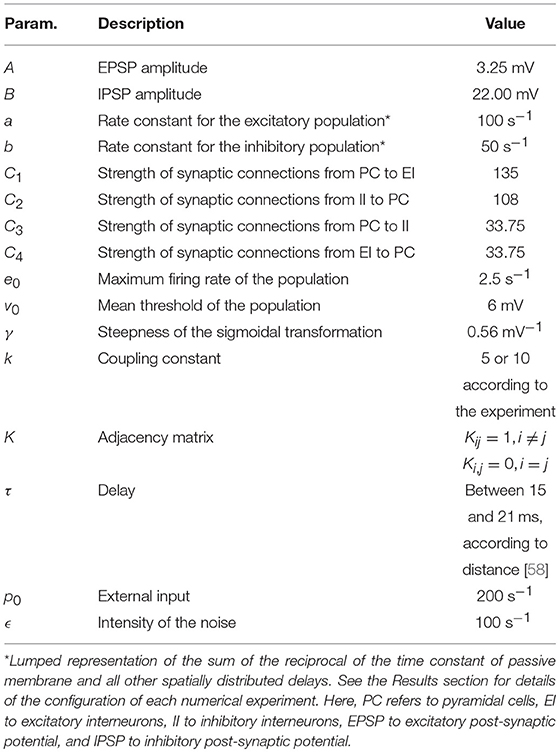
Table 1. Description and default values of the parameters for the system of neural masses.

2.2. Head Model

The main contribution of this paper is the use of multichannel extracranial data to obtain information about the neuronal populations inside the brain using data assimilation. To accomplish this, we use synthetic EEG data generated in silico using Jansen and Rit's model and Ary's head model. To that end, we transform the output x(t) of the neural masses to EEG signals z(t) in the electrodes (see Figure 1). This transformation is mediated by a lead field matrix [47], which builds on the basic idea of calculating the electric potential caused by a dipole source [13] on a three-layer isotropic hemisphere of radius 1 [46, 60] that represents the three main tissues that impact brain activity readings (brain, skull, and scalp). The lead field matrix also contains information about the geometry of the problem (e.g., locations of cortical columns and electrodes) and about the electrophysiology of the head (e.g., conductivities of the different tissues). The following equations show the potential V^e,i on an electrode e, located at r_e^e [61], caused by the dipole ${\text{q}}^i(t)=x^i(t){\widehat{q}}^i$ generated by the cortical column i, located at r_qⁱ and oriented as ${\widehat{q}}^i$. In these equations, e = 1, …, N_e, where N_e is the total number of electrodes, and i = 1, …, N_d, where N_d is the total number of dipoles. Vectors are typeset in bold and modules are in regular type.

$\begin{array}{l}{V}^{e,i}({\text{r}}_{\text{e}}^e;{\text{r}}_{\text{q}}^i,{\text{q}}^i)\approxeq v^1({\text{r}}_{\text{e}}^e;{\mu }_1{\text{r}}_{\text{q}}^i,{\rho }_1{\text{q}}^i)+v^2({\text{r}}_{\text{e}}^e;{\mu }_2{\text{r}}_{\text{q}}^i,{\rho }_2{\text{q}}^i)\\ +v^3({\text{r}}_{\text{e}}^e;{\mu }_3{\text{r}}_{\text{q}}^i,{\rho }_3{\text{q}}^i),& (5)\end{array}$

$\begin{array}{l}{v}^1(r_e^e;r_q^i,q^i)=((c_1^{e,i,1}-c_2^{e,i,1}(r_e^e·r_q^i))r_q^i+\\ c_2^{e,i,1}{(r_q^i)}^2{r}_e^e)·q^i,& (6)\end{array}$

$\begin{array}{l}{v}^2(r_e^e;r_q^i,q^i)=((c_1^{e,i,2}-c_2^{e,i,2}(r_e^e·r_q^i))r_q^i\\ +c_2^{e,i,2}{(r_q^i)}^2{r}_e^e)·q^i,& (7)\end{array}$

$\begin{array}{l}{v}^3(r_e^e;r_q^i,q^i)=((c_1^{e,i,3}-c_2^{e,i,3}(r_e^e·r_q^i))r_q^i\\ +c_2^{e,i,3}{(r_q^i)}^2{r}_e^e)·q^i.& (8)\end{array}$

In these expressions,

$\begin{array}{l}{c}_1^{e,i,s}=\frac{1}{4\pi {\sigma }^s{(r_q^i)}^2}\left(2\frac{d^{e,i}·r_q{ }^i}{{(d^{e,i})}^3}+\frac{1}{d^{e,i}}-\frac{1}{r_e^e}\right),\\ c_2^{e,i,s}=\frac{1}{4\pi {\sigma }^s{(r_q^i)}^2}\left(\frac{2}{{(d^{e,i})}^3}+\frac{d^{e,i}+r_e^e}{r_e\Gamma (r_e{ }^e,r_q{ }^i)}\right),\\ \Gamma (r_e{ }^e,r_q{ }^i)=d^{e,i}\left(r_e^e{d}^{e,i}+{(r_e^e)}^2-(r_q{ }^i·r_e{ }^e)\right).& (9)\end{array}$

FIGURE 1

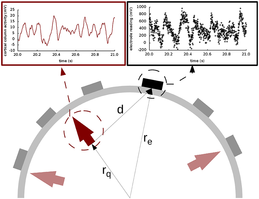
Figure 1. Extracranial data generation and illustration of Ary's model of the head. The light and dark red arrows indicate dipole sources, and the electrodes are shown as gray and black rectangles. The elements in the cartoon illustrate how all the signals produced by the cortical columns (represented with the solid red line in the top left panel) are transformed into an electrode reading (shown in black dots in the top right panel) through the lead field matrix. In this drawing, as in Equations (5–9), r_q is the distance from the origin to the cortical column under consideration; r_e is the distance from the origin to the electrode; and d is the distance from the cortical column to the electrode. The placement of the arrows here is for illustration purposes only; in our study, the cortical columns are placed on the surface of the brain, close to the skull.

The tangential conductivity of each layer is represented by σ^s [60] and ρ_s and μ_s are the Berg parameters relative to it [62] (see Table 2). The parameter $d^{e,i}=r_e{ }^e-r_q{ }^i$ is the relative position of the electrode e under consideration with respect to the position of the dipole i.

TABLE 2

Table 2. Values of the Berg parameters for the three layers [60, 62].

TABLE 3

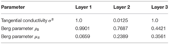
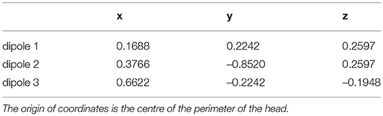
Table 3. Cartesian coordinates of the dipoles used throughout the study.

2.3. The Unscented Kalman Filter for Data Assimilation

The Unscented Kalman Filter (UKF) is our algorithm of choice to bring together the dynamical state of the model and the in silico data. It is a standard tool in the field of systems and control engineering, and has been shown to be both computationally efficient and robust even when dealing with stochastic nonlinear systems [63]. In our case, the computational burden—O(n³), where n is the size of the state—is acceptable for a biologically reasonable number of sources. In order to simultaneously estimate the state and parameters of the model described by Equations (1)–(3), we regard it as a discrete-time state-space dynamical system of the following form:

$\begin{array}{ll}{\text{x}}_{k+1}=\text{F}({\text{x}}_k)+{\text{v}}_k& (10)\end{array}$

$\begin{array}{ll}{\text{z}}_k=\text{H}({\text{x}}_k)+{\text{w}}_k& (11)\end{array}$

where $\text{x}=(x_0^1,x_1^1,x_2^1,x_0^2,\dots ,x_2^{N^d},{\theta }^1,\dots ,{\theta }^{N_p})\in {ℝ}^{n_x}$ is the state vector (related to the variables and parameters of the model), with θ^p being the parameters to estimate, which obey the equations ${\dot{\theta }}^p=0$. (In our joint estimation of the parameters, these are included in the state vector together with the system variables). The vector $\text{z}\in {ℝ}^{n_z}$ is the measurement vector (our in silico EEG readings). The vectors v and w are uncertainty terms that account for process noise and measurement noise, respectively, with Gaussian distributions p(v) ~N(0, Q) and p(w) ~N(0, R), respectively. The process transition F is obtained with a numerical implementation of Equations (1)–(3), as described below. Finally, H relates the state to measurement space, which is either V^{e, i} (in the case of simulated EEG), or xⁱ (in the case of simulated electrocorticography). Interestingly, where EEG is concerned, this basic part of the Kalman filter is in our case implemented by the skull, the effect of which is represented by the lead field matrix, based on Ary's head model and introduced above.

The UKF is a recursive predictor-corrector-type algorithm that aims to minimise the mean square error of the estimated states and parameters over time. For each time step it calculates a prediction of the state and parameters of the system, which is corrected when the information from a measurement is incorporated. The amount of confidence given to the model and measurement is quantified by the Kalman gain K, which is calculated at each time step based on prediction covariances as well as model and measurement error covariances (Q and R, respectively). For more details on the implementation of the filter, the reader is referred to the Appendix and to Kalman [54], Merwe and Wan [52], Julier and Uhlmann [53], and Solonen et al. [64].

2.4. Generation of in silico Datasets

For this paper three different in silico datasets were generated. We consider both simulated electrocorticography (ECoG, intracortical) and electroencephalography (EEG, extracranial) readings (using Ary's model in the latter case). We chose to use three sources because this provides a considerable spatial and temporal richness in the resulting signals, while keeping the system reasonably simple and still biologically plausible [65, 66].

The presence of additional dipoles in the brain, and its influence on the sources of study, is accounted for in the stochastic external input to the sources (p(t), see Equation 2):

$\begin{array}{ll}p(t)=p_0+\xi (t),& (12)\end{array}$

where $p_0=200{\text{s}}^{-1}$ and ξ(t) is Gaussian white noise [67] of zero mean and correlation 〈ξ(t)ξ(t′)〉 = 2ϵδ(t − t′) [68]. At the extracranial level, the other sources also affect the final EEG signal, as well as the different tissues (brain, skull, scalp, and even hair). This is modelled by adding Gaussian noise with zero mean and standard deviation 100 mV (unless otherwise stated) to the simulated EEG.

All datasets used the same locations for the cortical columns [66]. The electrodes were placed using a subset of the equidistant layout, a standard layout for EEG [69] (roughly illustrated in Figures 6–8). The strength of the coupling was set at a medium value so that the cortical columns have a visible effect on one another without fully synchronising behaviours and locking their dynamics (between k = 5 and k = 10), and the configurations of the couplings are as shown in Figure 2. Table 1 shows representative values for the parameters used in all analyses unless otherwise specified. In this paper we focus on estimating the amplitudes A of the EPSPs of the different cortical columns, and therefore we choose values for these amplitudes that produce signals that reflect various dynamic regimes that we wish to explore. (The rest of the parameters were fixed to their standard values [26, 51], as described in Table 1).

FIGURE 2

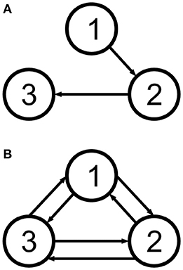
Figure 2. The two cortical column motifs used in this paper. Unidirectionally coupled cortical columns have no backflow (A), and bidirectionally coupled columns are coupled all-to-all (B). See Table 3.

The numerical solver used to generate the in silico time series was the Heun algorithm [70] with a time step of Δt = 1 ms. The length of the data is 100 s in all cases. Using the Heun algorithm together with Equations 1– 3 to update the state variables and the lead field matrix (in order to get the potential in the electrodes of the scalp in Equations 5– 9), we generate the required map to apply Kalman filtering in Equations 10 and 11. The following equations implement the stochastic Heun algorithm used to update x_k:

$\begin{array}{l}{\text{x}}_{k+1}={\text{x}}_k+\frac{1}{2}\left(\text{F}\left({\text{x}}_k\right)+\text{F}\left({\tilde{x}}_k\right)\right)\Delta t\\ +\frac{1}{2}\sum \left(g\left({\text{x}}_k\right)+g\left({\tilde{x}}_k\right)\right)X,& (13)\end{array}$

$\begin{array}{ll}{\tilde{x}}_k={\text{x}}_k+\text{F}({\text{x}}_k)\Delta t+g({\text{x}}_k)X.& (14)\end{array}$

Where g(…), together with Equation 12, introduces the noise term in Equation 2 and is zero for Equations 1 and 3. In $X=\sqrt{2ϵ\Delta t}\gamma$, γ are gaussianly distributed random numbers with zero mean and unit variance. At different instants of time, these random numbers are independent from one another.

2.4.1. Three Unidirectionally Coupled Cortical Columns

For the first study the cortical columns were coupled unidirectionally (Figure 2A), as described in Liu and Gao [71]. The parameters were set to standard values [26] for the three cortical columns (see Table 1), except for the first column, in which A₁ was set to 3.58 mV to make it hyperexcitable. Additionally, the three cortical columns had p₀ = 90 s⁻¹ and ϵ = 2 s⁻¹. This first hyperexcitable column causes a spiking cascade in the other two columns. With this experiment, we aimed to compare how extra- and intra-cranial electrodes perform in the case of a behaviour being induced by an input from another column, and not by the column's own parameter configuration. The resulting data can be found in the Data Sheets 1, 2 in Supplementary Material. Please, see the README file (Data Sheet 6) for more information.

2.4.2. Three Bidirectionally Coupled Cortical Columns: Coarse Parameter Estimation

The three cortical columns are located as in the previous section, but coupled bidirectionally (Figure 2B). Additionally, the maximum amplitudes of the excitatory PSPs were set to A₁ = 4.25 mV, A₂ = 10.00 mV, and A₃ = 3.25 mV. These values were chosen to cause the three cortical columns to be in very different dynamical regimes: cortical column 1 operates in a spiking regime; cortical column 2 oscillates with alpha frequency but with an amplitude similar to that of the spikes; and cortical column 3 oscillates in a more standard regime, as described in [26]. Also, the external input p(t) for each of the three cortical columns was set using $p_0=200{\text{s}}^{-1}$ and ϵ = 100 s⁻¹. Our aim here was to study how the filter performs in an extreme situation, in which the dynamics of the columns are widely different from one another. We intended to explore the outcome of estimating with single extracranial electrodes as well as the complete set, and to compare with intracranial estimation (Data Sheets 3, 4).

2.4.3. Three Bidirectionally Coupled Cortical Columns: Fine Parameter Estimation

In the previous section, the value of A of one of the cortical columns was much larger than the other two. We now consider the same coupling motif, but with values of the A parameter that are much closer together in value: A₁ = 3.58 mV, A₂ = 3.25 mV, and A₃ = 3.10 mV. (The values defining the external input p(t) remain the same as in the previous experiment). Our goal was to check if the filter can discriminate between the values when they are closer together (Data Sheet 5).

2.5. Filtering

For each of the experiments we conducted 50 realisations of each estimation for the complete state vector, with different initial conditions; all the figures show averages of the 50 estimations, unless otherwise specified. The initial conditions for state and parameter estimations were randomly generated with a normal distribution of zero mean and unit variance; the parameters, however, were constrained to deviate no more than 90% of their actual value as an initial assumption.

The noise covariances Q and R were chosen according to the best knowledge of the system and of the noise corrupting the data. Therefore, Q was set to contemplate the incoming noise to each dipole, i.e., it was set to a null matrix except for the term corresponding to the equation that contains the input p(t) (see Equation 2 and [68]). The matrix R was set to 1000I mV². (In practice, in most applications of the Kalman filter, the matrix R is fairly easy to set with the knowledge of the measurement precision as a starting point, but Q is often set by trial and error).

2.6. Ethics Statement

All data used in this manuscript come from numerical simulations of a mathematical model. No human or animal data have therefore been used, and ethics approval was not necessary.

3. Results

In order to compare the performance of the extra- and intra-cranial approaches to Kalman filtering, we have analysed three different cortical column configurations, each using one of the two motifs shown in Figure 2. Where relevant, two different types of estimations have been used: intracranial and extracranial. Intracranial estimation uses simulated data that would have hypothetically been obtained from electrocorticography, that is, using a single intracortical electrode, and is estimated with the data provided by a single location—in other words, the direct output of Jansen and Rit's model. Extracranial estimation, on the other hand, employs simulated data originated from EEG recordings, using several electrodes placed on the skull, and is implemented here with the projection on the head of the model output. We now discuss the results for the three different situations that we have considered.

3.1. Three Unidirectionally Coupled Cortical Columns

In this case, information flows unidirectionally because of the way the cortical columns are coupled [71]. As can be seen in the lower panels of Figure 3, the first cortical column has a random spiking activity, due to the increased value of A and the presence of noise [20]. Due to the architecture of the coupling, cortical column 1 causes cortical columns 2 and 3 to spike also, when otherwise they would have simply fluctuated around their resting level.

FIGURE 3

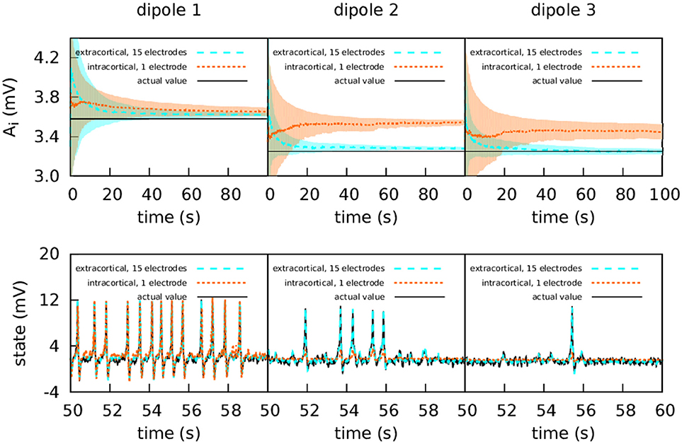
Figure 3. Intracranial and extracranial fittings with propagated excitation along unidirectionally coupled cortical columns. The upper panels show the estimation of parameter A, and the lower panels show the estimations of the observed states. The lines show the averages of the 50 realisations of the estimation, and the shadowed areas indicate the standard deviation. The actual values of the A parameters are A₁ = 3.58 mV, A₂ = 3.25 mV, and A₃ = 3.25 mV, the other parameters being set to standard values (Table 1). All three cortical columns received an external input, p(t), with $p_0=90{\text{s}}^{-1}$ and ϵ = 2 s⁻¹. The coupling constant was set to k = 10. The measurements were corrupted with Gaussian noise of mean 0 and standard deviation 100 mV for extracranial measurements and standard deviation 5 mV for intracortical measurements. Except for cortical column 1, with intracortical data the filter converges to a much higher value than the target, whereas with extracranial data the filter converges to a value which is accurate. In the lower panels it is shown that extracranial estimations of the state are also accurate, whereas intracortical estimations fail to reproduce the spikes correctly.

The upper panels of Figure 3 show the intracortical and extracranial estimations of A for the three cortical columns. The estimation for A₁ of the first column converges to its correct value, with both the intra- and extracortical approaches. This was to be expected, since the first cortical column receives no inputs from other elements of the system. In contrast, the intracortical estimations for cortical columns 2 and 3 converge to values significantly higher than their actual value of 3.25 mV. We conjecture that this is caused by the spiking of these two cortical columns, which as mentioned above is due to the influence of cortical column 1. Multi-channel extracranial information, in contrast, allows to see the complete picture of the coupled cortical columns and treat them as a single composed system, contrary to the partial picture obtained from the information provided by the single intracranial recordings. Therefore, estimation is better when using extracranial information with several electrodes, as shown in the upper panels of the figure. The lower panels of Figure 3 show the estimation of the state. The UKF shows great efficacy when the estimation is extracranial, but performs poorly in the case of intracortical estimation (with the exception of cortical column 1, because it has no input from other cortical columns). This highlights the value of extracranial estimation, in which it is possible to take the whole brain into account in a non-invasive manner.

3.2. Three Bidirectionally Coupled Cortical Columns: Coarse Parameter Estimation

The second experiment aims to explore the possibilities of the filter in more extreme situations, as the parameters were chosen to reflect more diverse dynamical regimes. The following sections describe the results of single- and multichannel estimations.

3.2.1. Moderate Intracortical Measurement Noise

Figure 4 shows again the performance obtained using the simulated data from a set of extracranial electrodes compared to using individual intracortical electrodes for each cortical column. In this case we show the 50 realisations of each filtering, without showing the average. The extracranial data for this experiment were corrupted with a measurement Gaussian noise of zero mean and standard deviation 100 mV; the intracortical data were corrupted with a measurement noise of standard deviation 5 mV in order to maintain similar levels of signal-to-noise ratio.

FIGURE 4

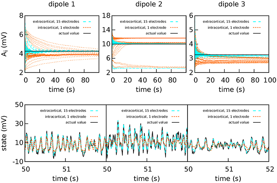
Figure 4. Intracranial and extracranial fittings for coarse parameter estimation in the case of bidirectional coupling. As in the previous figure, the upper panels show the estimation of A for each cortical column and the lower show the estimations of the observed states. The results are shown here without averaging. The actual values of the amplitudes of the EPSPs are A₁ = 4.25 mV, A₂ = 10.00 mV, and A₃ = 3.25 mV; the rest of the parameters were set to standard values (Table 1). The external input p(t) for the three cortical columns had p₀ = 200 s⁻¹ and ϵ = 100 s⁻¹. The coupling constant was set to k = 5. The intracortical measurements were corrupted with Gaussian noise of mean 0 and standard deviation 5 mV, while the noise in the extracranial measurements has standard deviation 100 mV. Extracranial estimations of the parameters are both faster and more accurate than intracortical estimations; this applies also to the state, whose dynamics are more faithfully reproduced using multi-electrode extracranial estimation (as shown in the lower panels).

As shown in Figure 4, the intracortical parameter estimations do not approximate the target value very well. In particular, the estimations of A for cortical column 2 converge to three different values depending on the initial conditions. The state estimation follows the actual state of the system closely only for cortical column 1. The situation is very different when with extracranial electrodes, where all 50 realisations of the estimations converge with much more precision to the correct values for both state and parameters (with the exception of A₂, which still tends to lower values in a very small quantity of the realisations). Again, extracranial performance is better, in general, to intracortical.

3.2.2. High Intracortical Measurement Noise

The difference between intracranial and extracranial estimation is even larger for higher measurement noise (Figure 5). In this case, the amount of noise in the intracortical data was set to the same value as the noise in the extracranial data. The value of R was tuned to reflect the increase in measurement noise, but the intracortical estimations failed to obtain the correct values for the parameters and reproduce the state.

FIGURE 5

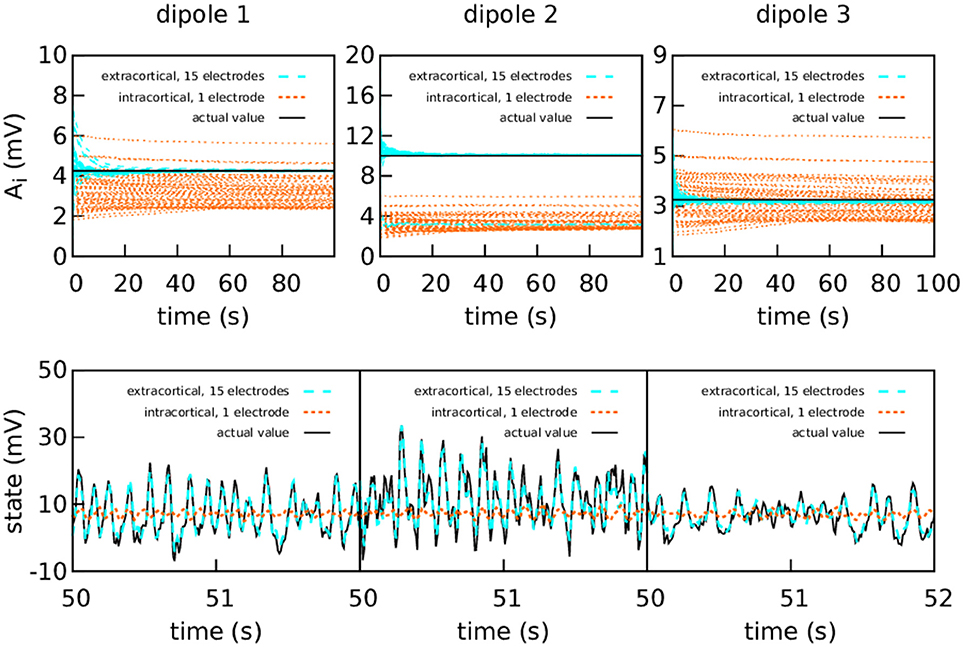
Figure 5. Intracranial and extracranial fittings for coarse parameter estimation, with a higher amount of intracortical measurement noise. The upper panels show the estimation of the EPSPs for each cortical column and the lower panels show the estimations of the observed states. The results are shown here without averaging. The actual values of the amplitudes of the EPSPs are A₁ = 4.25 mV, A₂ = 10.00 mV, and A₃ = 3.25 mV; the rest of the parameters were set to standard values (Table 1). The external input p(t) for the three cortical columns had $p_0=200{\text{s}}^{-1}$ and ϵ = 100 s⁻¹. The coupling constant was set to k = 5. The intracortical measurements were corrupted with Gaussian noise of mean 0 and standard deviation 100 mV—about an order of magnitude higher than the noise in the previous graph—, while the noise in the extracranial measurements has standard deviation 100 mV. Extracranial estimations of the parameters are also faster and more accurate than intracortical estimations, more markedly so in this case; as to the state, in this more extreme case, the intracortical estimation does not mimic the evolution of the system in any way.

3.2.3. Using One Single Extracranial Electrode

Using the same dataset, we aimed to investigate the outcome of using each extracranial electrode individually [43], as opposed to using the complete subset as until now. Therefore, we used each electrode separately to estimate the state and parameters of the complete system, with 50 realisations of the estimation for each electrode. By doing so, we show that the quality of the estimations is strongly dependent on the relative positions of sources and electrodes.

In Figures 6–8 we present the results for the estimation of parameter A of each of the three cortical columns separately. The histograms show the distribution of the 50 estimations of A using each electrode, placed in the respective position of the electrode in question. Vertical coloured lines in the histograms mark the value of the three A parameters being estimated (one in each figure). The histograms show a strong dependence on space of the quality of the estimations. As a general trait, the estimations are better when the electrodes are near the cortical column whose value of A is being estimated, whereas the more distant electrodes show a wider distribution of final values for the parameter.

FIGURE 6

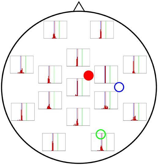
Figure 6. Distribution of 50 realisations of A estimations from a single electrode for cortical column 1 (solid red circle). The histograms are placed at the location of the corresponding measuring electrode, and the location of the three cortical columns generating the activity are shown with coloured circles (with the full circle corresponding to the column whose value of A is being estimated in this figure). Vertical lines with the same colours as the circles mark the corresponding actual A values. The distributions tend to be narrowest in the vicinities of cortical column 1. Nevertheless, they do not group around the target value of A₁ = 4.25 mV (vertical red line), as they should, but around that of A₃ = 3.25 mV (vertical blue line).

In Figure 6 the distribution of the estimations of A₁ are shown. The distributions tend to be narrowest in the vicinities of the cortical column whose A value is being estimated. However, it is noteworthy that the histograms obtained from the observations in distant electrodes tend to group not around the actual value of A₁ = 4.25 mV (red vertical line), but of A₃ = 3.25 mV (blue vertical line). This result suggests that the algorithm is unable to distinguish the origin of the EEG activity when sources and electrodes are distant from each other.

Figure 7 shows the results of the estimation of A₂ (actual value shown by vertical green lines), revealing wider distributions in general, which indicates a stronger dependence on initial conditions. Although it is true that the electrodes near cortical column 2 perform better in estimating A for that column, the difference with more distant electrodes is not as large as for the estimates of A for cortical columns 1 and 3.

FIGURE 7

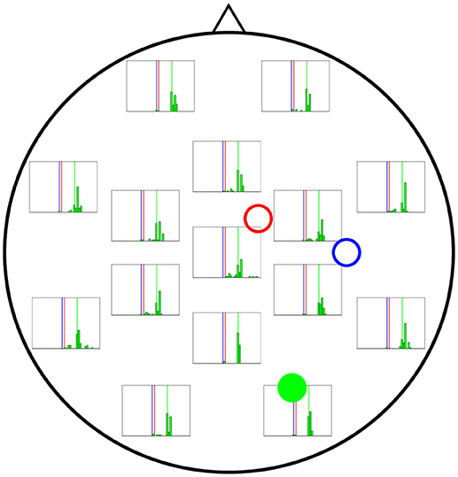
Figure 7. Distribution of 50 realisations of A estimations from a single electrode for cortical column 2 (solid green circle). The distributions here are wider than for A₁ and A₃, although they still tend to be more accurate near the cortical column (solid green circle) and group around the target value of A₂ = 10.00 mV (vertical green line).

Finally, Figure 8 shows the performance of each electrode when A₃ is being estimated (actual value shown by vertical blue lines in the figure). Interestingly, even the electrodes located at the far left of the figure lead to a good estimate of A, comparable to that coming from the electrodes in the far right, which are closer to column 3 and could therefore be expected to provide a much more accurate estimation.

FIGURE 8

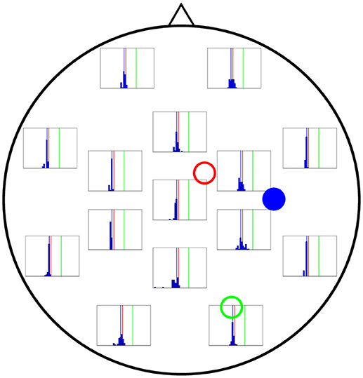
Figure 8. Distribution of 50 realisations of A estimations from a single electrode for cortical column 3 (solid blue circle). As in the two previous figures, the distributions for the electrodes closest to the source (solid blue circle) are narrow, grouping around the correct value (A₃ = 3.25 mV, vertical blue line). Surprisingly, the electrodes in the far left also give rise to narrow distributions.

While the estimations arising from single electrodes are reasonably accurate in some cases, using the complete set of 15 electrodes invariably yields better results. This is because, in Kalman filtering, combining many sources of information always improves the final estimation, even if some of the sources are inaccurate or incomplete [72].

3.3. Three Bidirectionally Coupled Cortical Columns: Fine Parameter Estimation

In the previous section, the aim was to generate widely different dynamics in each column. We now consider the results of estimating parameters which are much closer to one another. The purpose of this test was to ascertain whether the filter could differentiate between parameters with smaller differences in value. This ability is very important if we expect to use the technique in clinical applications. Figure 9 shows the extracranial estimation of the A parameters using the complete subset of 15 electrodes. The estimations converge to the actual values with enough accuracy as to give hopes of using the filter in a clinical setting.

FIGURE 9

Figure 9. Extracranial fit with parameters close together in value. The estimations of the amplitude of the EPSPs of the three cortical columns are shown after averaging over 50 realisations (solid lines); the shadowed areas indicate the standard deviation. The actual values of the amplitudes of the EPSPs are A₁ = 3.58 mV, A₂ = 3.25 mV, and A₃ = 3.10 mV; the rest of the parameters were set to standard values (Table 1). The external input p(t) for the three cortical columns had $p_0=200{\text{s}}^{-1}$ and ϵ = 100 s⁻¹. The coupling constant was set to k = 5. The Gaussian noise in the extracranial measurements has standard deviation 100 mV. The estimation of the parameters is fairly accurate.

4. Discussion

The most important limitation of current data assimilation processes in neuroscience is that the appropriate experimental recordings are usually intracranial. Despite this fact, using Kalman filtering to fit these data to neural mass models shows promise in several contexts and applications. In this study we have modified this type of approach by extending it with a head model, with the aim of integrating non-invasive experimental recordings taken from the scalp (EEG). By increasing the range of recordings in this way, the application of the data assimilation protocols opens up to the large set of situations in which scalp recordings are used. We keep the exploration of the technique using real EEG experimental data in mind, but here we have explored the limitations and advantages of our model using in silico data in very well controlled conditions.

Our main goal in this paper has been to show that data assimilation employing multiple non-invasive EEG electrodes (as coming from scalp EEG measurements) provides a better estimate of the brain's dynamical state than using a single invasive (intracranial) EEG electrode. In particular, we have aimed at contrasting our results with existing work using the latter approach, which has employed a filtering method, namely the unscented Kalman filter [39]. Filtering methods have been so far the method of choice in data assimilation problem in neuroscience [37, 38, 40–43], with variational methods having been used very sparsely [73]. We thus chose to work with a filtering algorithm, the UKF, that is already relatively well characterized in neural model, and which we could therefore use as a benchmark.

We have considered a system comprised of three cortical columns, modelled according to Jansen and Rit's equations and coupled following two different motifs. The cortical columns are all driven by a noisy input coming from the columns of the rest of the brain and sensory stimuli. The signal from the cortical columns is then transferred to the skull, after which it is corrupted with Gaussian noise to simulate electrode readings from EEG. These are then used to estimate the amplitude of the excitatory post-synaptic potentials.

Even though the quality of the experimental measurements at the scalp might be, in general, worse than the intracranial recordings, EEG can always be measured from several positions. This allows to obtain measurements for patients without intracranial implants and also to compensate the potentially low quality of the data by having many recordings at the same time. Besides, the spatial distribution of the electrodes on the scalp allows the information arriving from the whole cortex to be available during the assimilation process. In order to address these strengths and weaknesses of the scalp recordings with respect to intracranial measurements, we have analysed situations where assimilation with only intracortical recordings may be wanting, where diverse dynamical regimes coexist due to large differences in control parameters in the cortical columns, or where fine changes of the parameters make the discrimination difficult.

The first study considered here involves three columns that are coupled unidirectionally with no backflow. The first cortical column is made hyperexcitable by increasing the excitatory post-synaptic potential to A₁ = 3.58 mV; this cortical column causes the second cortical column and, indirectly, the third, to modify their behaviour by inducing spiking. For the intracranial estimations, single intracortical electrodes measured the evolution of the three cortical columns independently; for the extracranial estimations, 15 extracranial electrodes were used simultaneously. Applying the Kalman filter to the extracranial data provided a good estimation of the A parameters and of the dynamical state of the model; the intracortical measurements, however, yielded mixed results. The estimation for cortical column 1 was accurate, whereas for cortical columns 2 and 3 the estimation of A was above the target value and very close to the estimation for cortical column 1 (see orange dashed lines in Figure 3). The estimation of the dynamical state of cortical columns 2 and 3 was also worse than the estimation for cortical column 1. We attribute this to the fact that columns 2 and 3 are excited by column 1, which spikes due to a higher value of A. As a consequence, when independently evaluated using the intracranial information, the estimation is higher than the actual value. Therefore we suggest that one intracranial electrode provides only a partial view of the system, and thus cannot capture the behaviours of all three cortical columns and the interactions between them; the use of many electrodes provides a more complete view of the system.

Next we considered a situation in which the dipoles were coupled bidirectionally in an all-to-all configuration. The A parameters were chosen such as to cause different dynamic behaviours in the cortical columns. Three types of fitting via Kalman filtering were performed, using (i) independent intracortical recordings of single cortical columns, (ii) the complete subset of 15 extracranial electrodes, and (iii) single extracranial electrodes. The intracortical data were corrupted with two different levels (medium and high) of measurement noise. For both cases, the multi-electrode extracranial estimation surpasses the intracortical results in both speed of convergence and quality; the difference, however, is more marked in the presence of higher measurement noise in the intracortical recordings. In all these cases, the representation of the dynamical state of the three cortical columns using the complete set of 15 extracranial electrodes nicely matched the actual dynamical state, contrary to the limited match obtained using single intracranial or extracranial recordings. The results for the single electrodes show a significant influence of space on the quality of the estimations, in the sense that estimations of electrodes close to the source are relatively accurate, and electrodes further away from the source might not allow to discriminate the source of the information correctly, or might completely fail to represent the system.

Finally, we considered the situation of an identical cortical column configuration—in terms of situation and coupling—, except for the values of the EPSPs of the cortical columns. This dataset was filtered only extracranially, with the purpose of evaluating the filter's ability to discriminate parameter values within narrower ranges. The results in this case were also reasonably good, even though the real values of the parameter were much closer to one another, which makes data assimilation more challenging.

Even though the results shown here are better when considering extracranial electrodes, the method has, of course, limitations. For instance, the head model introduces new parameters which should be realistic. The use of Jansen's model, while being a very standard choice in the field, is not mandatory and could be substituted by others. There several alternatives to Ary's head model too. The succesful application of the method with different combinations of these models will, for sure, guide researchers to choose which models are more suitable for the theoretical description of the mesoscale in the brain. Even though the exploration of the dynamics for the different neural mass models or of the different head models might be worth exploring in future works, it lays outside of the scope of this work.

Applications of the method presented here will certainly appear in the field of brain-machine interface, long-term tracking for early diagnosis of degenerative diseases, or short-term tracking during rehabilitation of traumas and strokes. However, the succesful application of the method in each of these fields will require further research.

Taken as a whole, our results show that, independently of the need to explore more realistic situations, extracranial EEG recordings constitute a good candidate to be used together with neural mass models and Kalman filters, provided the method is extended with a head model. With its management of the noise in the system and of the inherent simplifications in neurological models, the Kalman filter is an appropriate tool for tackling the challenges of brain data processing. Using non-invasive techniques in these processes widens the applications of Kalman-based data assimilation methods in neuroscience.

Author Contributions

All authors listed have made a substantial, direct and intellectual contribution to the work, and approved it for publication.

Funding

This work was partially supported by the Spanish Ministry of Economy and Competitiveness and FEDER (project FIS2015-66503) and by the Catalan Government (AGAUR grant FI-DGR 2014-2017). JG-O also acknowledges support from the Catalan Government (project 2014SGR0947), the ICREA Academia programme, and from the María de Maeztu programme for Units of Excellence in R&D (Spanish Ministry of Economy and Competitiveness, MDM-2014-0370).

Conflict of Interest Statement

The authors declare that the research was conducted in the absence of any commercial or financial relationships that could be construed as a potential conflict of interest.

Acknowledgments

The authors wish to thank Drs. Maciej Jedynak and Daniel Malagarriga for helpful discussions.

Supplementary Material

The Supplementary Material for this article can be found online at: https://www.frontiersin.org/articles/10.3389/fams.2018.00046/full#supplementary-material

References

1. Yuste R. From the neuron doctrine to neural networks. Nature Rev Neurosci. (2015) 16:487–97. doi: 10.1038/nrn3962

PubMed Abstract | CrossRef Full Text | Google Scholar

2. Braitenberg V, Schütz A. Anatomy of the cortex. In: Statistics and Geometry, No. 18 in Studies of Brain Function. Berlin: Springer (1991).

Google Scholar

3. Izhikevich EM, Edelman GM. Large-scale model of mammalian thalamocortical systems. Proc Natl Acad Sci USA. (2008) 105:3593–8. doi: 10.1073/pnas.0712231105

PubMed Abstract | CrossRef Full Text | Google Scholar

4. Callaway EM. Micro-, Meso- and Macro-Connectomics of the Brain. Springer (2016). Available online at: http://link.springer.com/10.1007/978-3-319-27777-6

Google Scholar

5. Freeman WJ. Simulation of chaotic EEG patters with a dynamic model of the olfactory system. Biol Cybern. (1987) 56:139–50. doi: 10.1007/BF00317988

PubMed Abstract | CrossRef Full Text | Google Scholar

6. Faure P, Korn H. Is there chaos in the brain? I. Concepts of nonlinear dynamics and methods of investigation. C R Acad Sci III. (2001) 324:773–93. doi: 10.1016/S0764-4469(01)01377-4

PubMed Abstract | CrossRef Full Text | Google Scholar

7. Shadlen MN, Newsome WT. Noise, neural codes and cortical organization. Curr Opin Neurobiol. (1994) 4:569–79. doi: 10.1016/0959-4388(94)90059-0

PubMed Abstract | CrossRef Full Text | Google Scholar

8. Faisal AA, Selen LPJ, Wolpert DM. Noise in the nervous system. Nature Rev Neurosci. (2008) 9:292–303. doi: 10.1038/nrn2258

PubMed Abstract | CrossRef Full Text | Google Scholar

9. Schiff SJ, Jerger K, Duong DH, Chang T, Spano ML, Ditto WL. Controlling chaos in the brain. Nature (1994) 370:615–20. doi: 10.1038/370615a0

PubMed Abstract | CrossRef Full Text | Google Scholar

10. van Vreeswijk C, Sompolinsky H. Chaos in neuronal networks with balanced excitatory and inhibitory activity. Science (NY) (1996) 274:1724–6. doi: 10.1126/science.274.5293.1724

PubMed Abstract | CrossRef Full Text | Google Scholar

11. Celletti A, Froeschle C, Tetko IV, Villa AEP. Deterministic behaviour of short time series. Meccanica. (1999) 34:147–54. doi: 10.1023/A:1004668310653

CrossRef Full Text | Google Scholar

12. Stam CJ. Nonlinear dynamical analysis of EEG and MEG: review of an emerging field. Clin Neurophysiol. (2005) 116:2266–301. doi: 10.1016/j.clinph.2005.06.011

PubMed Abstract | CrossRef Full Text | Google Scholar

13. Buzsáki G, Anastassiou Ca, Koch C. The origin of extracellular fields and currents–EEG, ECoG, LFP and spikes. Nat Rev Neurosci. (2012) 13:407–20. doi: 10.1038/nrn3241

PubMed Abstract | CrossRef Full Text | Google Scholar

14. Wright JJ, Liley DTJ. Dynamics of the brain at global and microscopic scales: neural Networks and the EEG. Behav Brain Sci. (1996) 19:285. doi: 10.1017/S0140525X00042679

CrossRef Full Text | Google Scholar

15. Rabinovich MI, Varona P, Selverston AI, Abarbanel HDI. Dynamical principles in neuroscience. Rev Modern Phys. (2006) 78:1213. doi: 10.1103/RevModPhys.78.1213

CrossRef Full Text | Google Scholar

16. Eliasmith C, Stewart TC, Choo X, Bekolay T, DeWolf T, Tang C, et al. A large-scale model of the functioning brain. Science (2012) 338:1202–5. doi: 10.1126/science.1225266

PubMed Abstract | CrossRef Full Text | Google Scholar

17. Deco G, Ponce-Alvarez A, Hagmann P, Romani G, Mantini D, Corbetta M. How local excitation-inhibition ratio impacts the whole brain dynamics. J Neurosci. (2014) 34:7886–98. doi: 10.1523/JNEUROSCI.5068-13.2014

PubMed Abstract | CrossRef Full Text | Google Scholar

18. Nogaret A, Meliza CD, Margoliash D, Abarbanel HDI. Automatic construction of predictive neuron models through large scale assimilation of electrophysiological data. Sci Rep. (2016) 6:32749. doi: 10.1038/srep32749

PubMed Abstract | CrossRef Full Text | Google Scholar

19. David O, Friston KJ. A neural mass model for MEG/EEG: coupling and neuronal dynamics. Neuroimage (2003) 20:1743–55. doi: 10.1016/j.neuroimage.2003.07.015

PubMed Abstract | CrossRef Full Text | Google Scholar

20. Grimbert F, Faugeras O. Bifurcation analysis of Jansen's neural mass model. Neural Comput. (2006) 18:3052–68. doi: 10.1162/neco.2006.18.12.3052

PubMed Abstract | CrossRef Full Text | Google Scholar

21. Cona F, Zavaglia M, Massimini M, Rosanova M, Ursino M. A neural mass model of interconnected regions simulates rhythm propagation observed via TMS-EEG. Neuroimage (2011) 57:1045–58. doi: 10.1016/j.neuroimage.2011.05.007

PubMed Abstract | CrossRef Full Text | Google Scholar

22. Coombes S. Large-scale neural dynamics: Simple and complex. Neuroimage (2010) 52:731–9. doi: 10.1016/j.neuroimage.2010.01.045

PubMed Abstract | CrossRef Full Text | Google Scholar

23. Babajani A, Soltanian-Zadeh H. Integrated MEG/EEG and fMRI model based on neural masses. IEEE Trans Biomed Eng. (2006) 53:1794–1801. doi: 10.1109/TBME.2006.873748

PubMed Abstract | CrossRef Full Text | Google Scholar

24. Babiloni F, Cincotti F, Babiloni C, Carducci F, Mattia D, Astolfi L, et al. Estimation of the cortical functional connectivity with the multimodal integration of high-resolution EEG and fMRI data by directed transfer function. Neuroimage (2005) 24:118–31. doi: 10.1016/j.neuroimage.2004.09.036

PubMed Abstract | CrossRef Full Text | Google Scholar

25. Bojak I, Oostendorp TF, Reid AT, Kötter R. Connecting mean field models of neural activity to EEG and fMRI data. Brain Topogr. (2010) 23:139–49. doi: 10.1007/s10548-010-0140-3

PubMed Abstract | CrossRef Full Text | Google Scholar

26. Jansen BH, Rit VG. Electroencephalogram and visual evoked potential generation in a mathematical model of coupled cortical columns. Biol Cybern. (1995) 73:357–66. doi: 10.1007/BF00199471

PubMed Abstract | CrossRef Full Text | Google Scholar

27. Wendling F, Bartolomei F, Bellanger JJ, Chauvel P. Epileptic fast activity can be explained by a model of impaired GABAergic dendritic inhibition. Euro J Neurosci. (2002) 15:1499–508. doi: 10.1046/j.1460-9568.2002.01985.x

PubMed Abstract | CrossRef Full Text | Google Scholar

28. David O, Harrison L, Friston KJ. Modelling event-related responses in the brain. Neuroimage (2005) 25:756–70. doi: 10.1016/j.neuroimage.2004.12.030

PubMed Abstract | CrossRef Full Text | Google Scholar

29. Spiegler A, Knösche TR, Schwab K, Haueisen J, Atay FM. Modeling brain resonance phenomena using a neural mass model. PLoS Comput Biol. (2011) 7:e1002298. doi: 10.1371/journal.pcbi.1002298

PubMed Abstract | CrossRef Full Text | Google Scholar

30. Wright JJ, Robinson PA, Rennie CJ, Gordon E, Bourke PD, Chapman CL, et al. Toward an integrated continuum model of cerebral dynamics: the cerebral rhythms, synchronous oscillation and cortical stability. BioSystems (2001) 63:71–88. doi: 10.1016/S0303-2647(01)00148-4

PubMed Abstract | CrossRef Full Text | Google Scholar

31. Schiff SJ, Sauer T. Kalman filter control of a model of spatiotemporal cortical dynamics. J Neural Eng. (2008) 5:1–8. doi: 10.1088/1741-2560/5/1/001

PubMed Abstract | CrossRef Full Text | Google Scholar

32. Kiebel SJ, Garrido MI, Moran RJ, Friston KJ. Dynamic causal modelling for EEG and MEG. Cogn Neurodyn. (2008) 2:121–36. doi: 10.1007/s11571-008-9038-0

PubMed Abstract | CrossRef Full Text | Google Scholar

33. Shine JM, Koyejo O, Bell PT, Gorgolewski KJ, Gilat M, Poldrack RA. Estimation of dynamic functional connectivity using Multiplication of Temporal Derivatives. Neuroimage (2015) 122:399–407. doi: 10.1016/j.neuroimage.2015.07.064

PubMed Abstract | CrossRef Full Text | Google Scholar

34. Ma X, Chou CA, Sayama H, Chaovalitwongse WA. Brain response pattern identification of fMRI data using a particle swarm optimization-based approach. Brain Informat. (2016) 3:181–92. doi: 10.1007/s40708-016-0049-z

PubMed Abstract | CrossRef Full Text | Google Scholar

35. Alswaihli J, Potthast R, Bojak I, Saddy D, Hutt A. Kernel reconstruction for delayed neural field equations. J Math Neurosci. (2018) 8:3. doi: 10.1186/s13408-018-0058-8

PubMed Abstract | CrossRef Full Text | Google Scholar

36. Voss HU, Timmer J, Kurths J. Nonlinear dynamical system identification from uncertain and indirect measurements. Int J Bifurcat Chaos (2004) 14:1905–33. doi: 10.1142/S0218127404010345

CrossRef Full Text | Google Scholar

37. Hamilton F, Berry T, Peixoto N, Sauer T. Real-time tracking of neuronal network structure using data assimilation. Phys Rev E. (2013) 88:052715. doi: 10.1103/PhysRevE.88.052715

PubMed Abstract | CrossRef Full Text | Google Scholar

38. Hamilton F, Cressman J, Peixoto N, Sauer T. Reconstructing neural dynamics using data assimilation with multiple models. EPL (Europhys Lett). (2014) 107:68005. doi: 10.1209/0295-5075/107/68005

CrossRef Full Text | Google Scholar

39. Freestone DR, Kuhlmann L, Chong MS, Nesic D, Grayden DB, Aram P, et al. Patient-specific neural mass modeling - stochastic and deterministic, methods. In: Recent Advances in Predicting and Preventing Epileptic Seizures. (2013) p. 63–82. Available online at: https://hal.archives-ouvertes.fr/hal-00876475/%5Cnhttp://www.worldscientific.com/doi/abs/10.1142/9789814525350_0005

Google Scholar

40. Shan B, Wang J, Deng B, Wei X, Yu H, Li H. UKF-based closed loop iterative learning control of epileptiform wave in a neural mass model. Cogn Neurodyn. (2015) 9:31–40. doi: 10.1007/s11571-014-9306-0

PubMed Abstract | CrossRef Full Text | Google Scholar

41. López-Cuevas A, Castillo-Toledo B, Medina-Ceja L, Ventura-Mejía C. State and parameter estimation of a neural mass model from electrophysiological signals during the status epilepticus. Neuroimage. (2015) 113:374–86. doi: 10.1016/j.neuroimage.2015.02.059

PubMed Abstract | CrossRef Full Text | Google Scholar

42. Li S, Li J, Li Z. An improved unscented kalman filter based decoder for cortical brain-machine interfaces. Front Neurosci. (2016) 10:587. doi: 10.3389/fnins.2016.00587

PubMed Abstract | CrossRef Full Text | Google Scholar

43. Freestone DR, Karoly PJ, Nešić D, Aram P, Cook MJ, Grayden DB. Estimation of effective connectivity via data-driven neural modeling. Front Neurosci. (2014) 8:383. doi: 10.3389/fnins.2014.00383

PubMed Abstract | CrossRef Full Text | Google Scholar

44. Cao Y, Ren K, Su F, Deng B, Wei X, Wang J. Suppression of seizures based on the multi-coupled neural mass model. Chaos (2015) 25:103120. doi: 10.1063/1.4931715

PubMed Abstract | CrossRef Full Text | Google Scholar

45. Kuhlmann L, Freestone DR, Manton JH, Heyse B, Vereecke HEM, Lipping T, et al. Neural mass model-based tracking of anesthetic brain states. Neuroimage (2016) 133:438–56. doi: 10.1016/j.neuroimage.2016.03.039

PubMed Abstract | CrossRef Full Text | Google Scholar

46. Zhang Z. A fast method to compute surface potentials generated by dipoles within multilayer anisotropic spheres. Phys Med Biol. (1995) 40:335–49. doi: 10.1088/0031-9155/40/3/001

PubMed Abstract | CrossRef Full Text | Google Scholar

47. Mosher JC, Leahy RM, Lewis PS. EEG and MEG: forward solutions for inverse methods. IEEE Trans Biomed Eng. (1999) 46:245–59. doi: 10.1109/10.748978

PubMed Abstract | CrossRef Full Text | Google Scholar

48. Haufe S, Tomioka R, Dickhaus T, Sannelli C, Blankertz B, Nolte G, et al. Large-scale EEG/MEG source localization with spatial flexibility. Neuroimage (2011) 54:851–9. doi: 10.1016/j.neuroimage.2010.09.003

PubMed Abstract | CrossRef Full Text | Google Scholar

49. Verhellen E, Boon P. EEG source localization of the epileptogenic focus in patients with refractory temporal lobe epilepsy, dipole modelling revisited. Acta Neurol Belg. (2007) 107:71–7. Available online at: http://www.actaneurologica.be/pdf.php?annee=2007&trimestre=3

PubMed Abstract | Google Scholar

50. Gotman J. Noninvasive methods for evaluating the localization and propagation of epileptic activity. Epilepsia. (2003) 44(Suppl 1):21–9. doi: 10.1111/j.0013-9580.2003.12003.x

PubMed Abstract | CrossRef Full Text | Google Scholar

51. Jansen BH, Zouridakis G, Brandt ME. A neurophysiologically-based mathematical model of flash visual evoked potentials. Biol Cybern. (1993) 68:275–83. doi: 10.1007/BF00224863

PubMed Abstract | CrossRef Full Text | Google Scholar

52. Merwe RVD, Wan EA. The square-root unscented Kalman filter for state and parameter-estimation. in: Proceedings of (ICASSP '01) 2001 IEEE International Conference on Acoustics, Speech, and Signal Processing, Vol. 6. Salt Lake City (2001). p. 3461–4.

Google Scholar

53. Julier SJ, Uhlmann JK. Unscented filtering and nonlinear estimation. Proc IEEE (2004) 92:401–22. doi: 10.1109/JPROC.2003.823141

CrossRef Full Text | Google Scholar

54. Kalman RE. A new approach to linear filtering and prediction problems. Trans ASME J Basic Eng. (1960) 82:35–45. doi: 10.1115/1.3662552

CrossRef Full Text | Google Scholar

55. Silva FHLD, Hoeks A, Smits H, Zetterberg LH. Model of brain rhythmic activity. Kybernetic (1974) 15:27–37. doi: 10.1007/BF00270757

CrossRef Full Text | Google Scholar

56. Faugeras O, Touboul J, Cessac B. A constructive mean-field analysis of multi-population neural networks with random synaptic weights and stochastic inputs. Front Comput Neurosci. (2009) 3:1. doi: 10.3389/neuro.10.001.2009

PubMed Abstract | CrossRef Full Text | Google Scholar

57. Grimbert F, Faugeras O. Analysis of Jansen's Model of a Single Cortical Column. Research Report INRIA (2006).

Google Scholar

58. Pons AJ, Cantero JL, Atienza M, Garcia-Ojalvo J. Relating structural and functional anomalous connectivity in the aging brain via neural mass modeling. Neuroimage (2010) 52:848–61. doi: 10.1016/j.neuroimage.2009.12.105

PubMed Abstract | CrossRef Full Text | Google Scholar

59. Silva FLD. 5. In: EEG: Origin and Measurement. World Scientific Publishing Co. (2011). p. 63–82. Available online at: http://www.worldscientific.com/doi/abs/10.1142/9789814525350_0005

Google Scholar

60. Ary JP, Klein SA, Fender DH. Location of sources of evoked scalp potentials: corrections for skull and scalp thicknesses. IEEE Trans Biomed Eng (1981) 28:447–52. doi: 10.1109/TBME.1981.324817

PubMed Abstract | CrossRef Full Text | Google Scholar

61. Jurcak V, Tsuzuki D, Dan I. 10/20, 10/10, and 10/5 systems revisited: their validity as relative head-surface-based positioning systems. Neuroimage (2007) 34:1600–11. doi: 10.1016/j.neuroimage.2006.09.024

PubMed Abstract | CrossRef Full Text | Google Scholar

62. Berg P, Scherg M. A fast method for forward computation of multiple-shell spherical head models. Electroencephalogr Clin Neurophysiol. (1994) 90:58–64. doi: 10.1016/0013-4694(94)90113-9

PubMed Abstract | CrossRef Full Text | Google Scholar

63. Merwe RVD, Wan EA. The unscented kalman filter for nonlinear estimation. In: Adaptive Systems for Signal Processing, Communications, and Control Symposium 2000, AS-SPCC. Lake Louise, CA: IEEE (2000). p. 153–8.

Google Scholar

64. Solonen A, Hakkarainen J, Ilin A, Abbas M, Bibov A. Estimating model error covariance matrix parameters in extended Kalman filtering. Nonlinear Process Geophys. (2014) 21:919–27. doi: 10.5194/npg-21-919-2014

CrossRef Full Text | Google Scholar

65. Cantero JL, Atienza M, Gomez-Herrero G, Cruz-Vadell A, Gil-Neciga E, Rodriguez-Romero R, et al. Functional integrity of thalamocortical circuits differentiates normal aging from mild cognitive impairment. Hum Brain Mapp. (2009) 30:3944–57. doi: 10.1002/hbm.20819

PubMed Abstract | CrossRef Full Text | Google Scholar

66. Richards JE. Recovering dipole sources from scalp-recorded event-related-potentials using component analysis: principal component analysis and independent component analysis. Int J Psychophysiol. (2004) 54:201–20. doi: 10.1016/j.ijpsycho.2004.03.009

PubMed Abstract | CrossRef Full Text | Google Scholar

67. Crispin W, Gardiner. Handbook of Stochastic Methods for Physics, Chemistry, and the Natural Sciences. Berlin: Springer (2004).

Google Scholar

68. Garcia-Ojalvo J, Sancho J. Noise in Spatially Extended Systems, 1999th Edn. New York, NY: Institute for Nonlinear Science, Springer (1999).

Google Scholar

69. Easycap. Easycap Equidistant Layouts. (2018). Available online at: https://www.easycap.de/wordpress/wp-content/uploads/2018/02/Easycap-Equidistant-Layouts.pdf

70. Toral R, Colet P. Stochastic Numerical Methods: An Introduction for Students and Scientists. John Wiley & Sons (2014).

Google Scholar

71. Liu X, Gao Q. Parameter estimation and control for a neural mass model based on the unscented Kalman filter. Phys Rev E. (2013) 88:042905. doi: 10.1103/PhysRevE.88.042905

PubMed Abstract | CrossRef Full Text | Google Scholar

72. Schiff SJ. Neural control engineering: the emerging intersection between control theory and neuroscience. In: Computational Neuroscience. MIT Press (2012). Available online at: https://books.google.es/books?id=P9UvTQtnqKwC

Google Scholar

73. Moye MJ, Diekman CO. Data assimilation methods for neuronal state and parameter estimation. J Math Neurosci. (2018) 8:11. doi: 10.1186/s13408-018-0066-8

PubMed Abstract | CrossRef Full Text | Google Scholar

Appendix: The Unscented Kalman filter (UKF) Algorithm

UKF is a predictor-corrector algorithm that estimates the state and parameters at a given time step k in two phases. The first one predicts the state based solely on the dynamical information of the system, i.e., the model. The second incorporates a measurement with which to correct the first estimation. Table A1 presents the symbols used in this paper for the variables of the Kalman filter.

TABLE A1

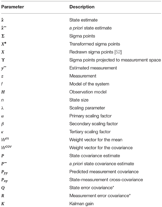
Table A1. Variables of the Unscented Kalman Filter.

The first step of the algorithm involves computing the expectation of the state and of the state covariance at time instant k + 1, known as the a priori estimation. For this we use a numerical implementation (using Heun's solver) of Jansen and Rit's model of a cortical column [26, 51], as described in the section 2.2.

The nature of the nonlinearities of this model prevents us from using a simple linearisation approach to propagating the statistics of the state variables across the transformation, as would be the case if we used the extended Kalman filter, for example. Therefore, we incorporate the unscented transform (UT) in our formulation of the Kalman filter, which, instead of attempting to propagate a distribution through the nonlinearity, first propagates a series of deterministically chosen points through the nonlinearity and then recovers the statistical information of the distribution from these.

Therefore, the a priori estimation of the state, ${\widehat{x}}_k^{-}$, is obtained as follows, beginning with the calculation and projection of the 2n + 1 (where n is the state size) sigma points,

$\begin{array}{l}{\Sigma }_{k-1,0}={\widehat{x}}_{k-1}\end{array}$

$\begin{array}{ll}{\Sigma }_{k-1,i}={\widehat{x}}_{k-1}+{\left(\sqrt{(n+\lambda )P_{k-1}}\right)}_i,i=1,\mathrm{...},n& (\text{A}1)\end{array}$

$\begin{array}{l}{\Sigma }_{k-1,i}={\widehat{x}}_{k-1}-{\left(\sqrt{(n+\lambda )P_{k-1}}\right)}_{i-n},i=n+1,\mathrm{...},2n\end{array}$

where P_k−1 is the estimated state covariance matrix for the previous time step. The square root of this matrix is well-defined, and can be calculated efficiently via a Cholesky decomposition [52]. This continues with the condensation of the projected sigma points into the a priori state estimate:

$\begin{array}{ll}{X}_{k|k-1}^{*}=f({\Sigma }_{k-1})& (\text{A}2)\end{array}$

$\begin{array}{ll}{\widehat{x}}_k^{-}={\displaystyle \sum _{i=0}^{2L}{W}_i^m}{X}_{i,k|k-1}^{*}& (\text{A}3)\end{array}$

$\begin{array}{ll}{P}_k^{-}={\displaystyle \sum _{i=0}^{2L}{W}_i^{cov}}[X_{i,k|k-1}^{*}-{\widehat{x}}_k^{-}]{[X_{i,k|k-1}^{*}-{\widehat{x}}_k^{-}]}^T+Q& (\text{A}4)\end{array}$

where Q is the state error covariance and W^m and W^cov are the weight vectors, defined as

$\begin{array}{l}{W}_0^m=\frac{\lambda }{n+\lambda }\end{array}$

$\begin{array}{ll}{W}_0^{cov}=\frac{\lambda }{n+\lambda }+1-{\alpha }^2+\beta & (\text{A}5)\end{array}$

$\begin{array}{l}{W}_i^m=W_i^{cov}=\frac{1}{2(n+\lambda )},i=1,\mathrm{...},2n\end{array}$

In Equations 1 and 5, α, β and κ are scaling factors, and λ, which is crucial to guarantee a positive semi-definite covariance matrix P, is calculated as λ = α²(n + κ) − n. The primary scaling factor α determines the spread of the sigma points around the mean and is set at 0.001, it being usually set between 0.001 and 1 [63] and chosen according to the quality of the resulting estimation. The secondary scaling factor β contains prior information about the distribution of x; for Gaussian distributions, its optimal value is 2. Finally, κ, the tertiary scaling parameter, is set to 0, as is a usual practice [63].

We now use a measurement to correct the state estimation, which implies the mapping of the a priori estimate onto the measurement space for comparison. In our case, this transformation is a linear matrix H that relates the state of the cortical columns to an EEG reading (see section 2.2 for details). The sigma points Σ_k|k−1 are projected into the measurement space [52]

$\begin{array}{ll}{{\rm Y}}_{k|k-1}=H[{\Sigma }_{k|k-1}],& (\text{A}6)\end{array}$

from which the estimation of the measurement, ${\widehat{y}}_k^{-}$, is calculated:

$\begin{array}{ll}{\widehat{y}}_k^{-}={\displaystyle \sum _{i=0}^{2L}{W}_i^m}{{\rm Y}}_{i,k|k-1}& (\text{A}7)\end{array}$

The second step of the algorithm corrects the a priori estimation of state and covariance by using the information available from the most recent measurement (in our case, an EEG reading). The impact of the measurement is determined by the Kalman gain K_k, which essentially expresses the level of confidence on the accuracy of the model and the level of noise in the data.

$\begin{array}{ll}{P}_{y_k{y}_k}={\displaystyle \sum _{i=0}^{2L}{W}_i^{cov}}[{{\rm Y}}_{i,k|k-1}-{\widehat{y}}_k^{-}]{[{{\rm Y}}_{i,k|k-1}-{\widehat{y}}_k^{-}]}^T+R& (\text{A}8)\end{array}$

$\begin{array}{ll}{P}_{x_k{y}_k}={\displaystyle \sum _{i=0}^{2L}{W}_i^{cov}}[X_{i,k|k-1}-{\widehat{x}}_k^{-}]{[{{\rm Y}}_{i,k|k-1}-{\widehat{y}}_k^{-}]}^T& (\text{A}9)\end{array}$

$\begin{array}{ll}{K}_k=P_{x_k{y}_k}{{\displaystyle P_{y_k{y}_k}}}^{-1}& (\text{A}10)\end{array}$

$\begin{array}{ll}{\widehat{x}}_k={\widehat{x}}_k^{-}+K_k(z_k-{\widehat{y}}_k^{-})& (\text{A}11)\end{array}$

$\begin{array}{ll}{P}_k=P_k^{-}-K_k{P}_{y_k{y}_k}{{\displaystyle K_k}}^T& (\text{A}12)\end{array}$

where P_ykyk is the predicted measurement covariance, P_xkyk is the state-measurement cross-covariance, R is the measurement error covariance, and z_k is the measurement for the current time step.