 Axel Hutt1,2*
 Roland Potthast1,2
- 1Department FE12 - Data Assimilation, Deutscher Wetterdienst, Offenbach, Germany
- 2Department of Applied Mathematics and Statistics, University of Reading, Reading, United Kingdom
Data assimilation permits to compute optimal forecasts in high-dimensional systems as, e.g., in weather forecasting. Typically such forecasts are spatially distributed time series of system variables. We hypothesize that such forecasts are not optimal if the major interest does not lie in the temporal evolution of system variables but in time series composites or features. For instance, in neuroscience spectral features of neural activity are the primary functional elements. The present work proposes a data assimilation framework for forecasts of time-frequency distributions. The framework comprises the ensemble Kalman filter and a detailed statistical ensemble verification. The performance of the framework is evaluated for a simulated FitzHugh-Nagumo model, various measurement noise levels and for in situ-, nonlocal and speed observations. We discover a resonance effect in forecast errors between forecast time and frequencies in observations.
1. Introduction
Understanding the dynamics of natural complex systems is one of the great challenges in science. Various research domains have developed optimized analytical methods, computational techniques or conceptual frameworks to gain deeper insight into the underlying mechanisms of complex systems. In the last decades, more and more interdisciplinary research attracted attention building bridges between research domains by applying methodologies outside of domains. These cross-disciplinary techniques fertilize research domains and shed new light on their underlying properties. A prominent example is the mathematical domain of dynamical systems theory that traditionally is applied in physics and engineering and that has been applied very successfully in biology and neuroscience. For instance, taking a closer look at the spatio-temporal nonlinear dynamics of neural populations has allowed to identify epilepsy as a so-called dynamical disease [1]. This approach explains epileptic seizures as spatio-temporal instabilities hypothesizing that epileptic seizures emerge by phase transitions well-studied in physics. Another example is control theory that is well-established in electric engineering, e.g., in the cruise-control in automobiles or the flight control of airplanes. Similar control engineering techniques have been applied in neuroscience for some years now, e.g., to optimize electric deep brain stimulation in Parkinson disease [2, 3].
Weather forecasts are an everyday service provided by national and regional weather services that allows to plan business processes as well as private activity and serves as a warning system for extreme weather situations, such as floods or thunderstorms. Weather forecast is also an important research domain in meteorology that has been developed successfully in the last decades improving the forecasts for both global phenomena and local weather situations. In detail, todays weather services employ highly tuned and optimized meteorological models and data processing techniques to compute reliable forecasts. Specifically the combination of an efficient model and measured meteorological data enables researchers to provide various types of predictions, such as the probability of rain or the expected temperature in certain local regions. This optimal combination of model and data is achieved by data assimilation [4] and yields corresponding optimal forecasts.
In other research domains, prediction methods are rare but highly requested. For instance, the prediction of epileptic seizures [5] would dramatically improve the life of epilepsy patients and spare some of them health-critical drug treatments. The typical approach of seizure prediction classifies measured neural activity [6, 7] into seizure-no seizure data, what however does not provide forecasts of neural activity. Although such forecasts are made possible by data assimilation techniques, until today research in neuroscience does apply data assimilation rarely. In recent years, data assimilation methods have been applied in neuroscience for model parameter identification primarily [3, 8–12]. The present work extends these studies by a framework to both compute and validate forecasts in neural problems. Although large parts of the methodology presented is well-established in meteorological forecasts [4], we extend the techniques by a focus on spectral features in measurement data. Such spectral data features play an important role in neuroscience since there is almost-proofed evidence that neural information processing is encoded in rhythmic activity. For instance, mammalian visual perception is achieved by synchronization in the frequency range [30 Hz;60 Hz] [13] and unconsciousness and sleep is reflected in increased activity in the frequency range [0.5 Hz;4 Hz] [14]. Moreover, epileptic seizures exhibit strong rhythmic patterns [1]. Consequently, we aim to forecast spectral distributions over time. To our best knowledge the present work is one of the first to predict spectral distributions optimally by data assimilation.
Most recent data assimilation studies apply the unscented Kalman filter [3, 10] that performs well for low-dimensional models. The present work considers the ensemble Kalman filter [15, 16] that has been shown to outperform the unscented Kalman filter and still performs well for high-dimensional models [17]. One of the major differences to previous studies is that the data assimilation cycle applied here does not estimate system parameters but providing reasonable forecasts. We provide a detailed description of the data assimilation elements and its extension to spectral feature forecasts. The additional verification of the ensemble forecasts gives insights into the power and weakness of spectral feature forecasts. For instance, we find a resonance effect between forecast time and the oscillation frequency of observations that yields improved verification metrics although forecasts are not improved.
The work is structured as follows. The Methods section introduces the model, simulated observations, the ensemble Kalman filter and the verification metrics applied. The subsequent section shows obtained results for in situ-, nonlocal, and speed observations and various measurement noise levels. A final discussion closes the work.
2. Materials and Methods
2.1. The Model
Single biological neurons may exhibit various types of activity, such as no spike discharge, discharge of single spikes, regular spike discharge, or spike burst discharges. These activity modes can be described by high-dimensional dynamical models. A more simple model is the FitzHugh-Nagumo model [18, 19] describing spike discharges by two coupled nonlinear ordinary differential equations
with membrane potential V, recovery variable w and corresponding time scale τ , external input I, and physiological constants a = 0.1, b = −0.15. In our study, we consider two models. The nature model is non-homogeneous and time scales and input vary according to
with maximum time T. This model is supposed to describe the true dynamics in the system under study and typically that one does not know. The change of τn and In over time results in a shift of oscillation frequency of the system, i.e., from larger to smaller frequencies. Such a non-homogeneous temporal rhythm is well-known in neuroscience, e.g., in the presence of anesthetic drugs [20, 21]. The false model is not complete and represents just an estimate of the system under study. This is the model with which one describes systems and, typically, it is not correct. We assume that we do not know the non-homogeneous nature of the true model and assume temporally constant time scale and input
leading to a single oscillation frequency. We point out that τn(T) = τf and In(T) = If and both models converge to each other for t → T.
The model integration over time uses a time step of 0.01 and every 50 steps a sample is written out running the integration over 5·104 steps in total. Initial conditions are x(t = 0) = (1.0, 0.2)t. After numerical integration, we re-scaled the unit-less time by αt → t with α = 0.002s rendering the sample time to Δt = 1 ms and the maximum time to tmax = 1s. This sets the number of data points to N = 1, 000.
To reveal non-stationary cyclic dynamics, we analyze the time-frequency distribution of data with spectral density S(tk, νm), k = 1, …, K, m = 1, …, M for number of time points K and number of frequencies M. The Morlet wavelet transform
applied uses a mother wavelet Ψ with central frequency fc = 8 and the time-frequency distribution has a frequency resolution of Δν = 0.5 Hz in the range ν ∈ [5 Hz;20 Hz]. The parameter a = fc/ν is the scale that depends on the pseudo-frequency ν. By the choice of the central frequency fc, the mother wavelet has a width of 4 periods of the respective frequency. This aspect is important to re-call while interpreting temporal borders of time-frequency distributions. For instance, at a frequency of 15 Hz border disturbances occur in a window of 0.26 s from the initial and final time instant.
Figure 1A presents the phase space dynamics of the true model (black) and the false model (red) and one observes nonlinear cyclic dynamics. For illustration, Figure 1B shows the potential V. Oscillations of the true model (black) decelerate with time while the false model dynamics (red) is a stationary limit cycle. This can be seen even better in the time-frequency distribution shown in Figures 1C,D of the corresponding observations.
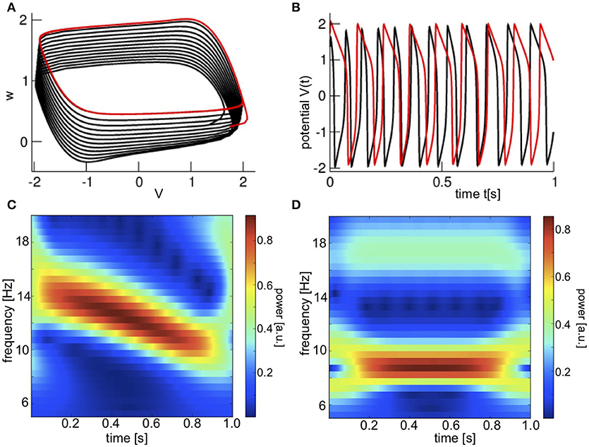
Figure 1. Noise-free dynamics of the Fitzhugh-Nagumo model and corresponding observations. (A) The model trajectory in phase space for non-stationary (black) and stationary (red) dynamics. (B) The time series of corresponding observations H[x] for non-stationary and stationary dynamics. (C) The time-frequency evolution of observations for non-stationary dynamics in the true model with Equation (2). (D) The time-frequency evolution of observations for the stationary dynamics with Equation (3).
2.2. Observations
To relate model variables to observations, data assimilation introduces the notion of a measurement operator . This operator maps system variables in model space to observable variables in observation space .
The system dynamics can be observed in various ways and the observation operator is chosen correspondingly. Measurements directly in the system are called in-situ observations and, typically, the measured observable is proportional to a model variable. In this case, the operator is proportional to the identity. Examples for such observables are temperature or humidity in meteorology and intra-cellular potentials or Local Field Potentials in neurophysiology. Conversely, measurements outside the system are called nonlocal observations capturing the integral of activity from the system. Examples for such observations are satellite radiances or radar reflectivities in meteorology and encephalographic data and the BOLD response in functional Magnetic Resonance Imaging in neurophysiology.
The present study considers scalar in-situ observations, nonlocal observations and temporal derivatives and in-situ observations. We begin with in-situ observations y(t) disturbed by measurement noise
where ξ(t) are Gaussian distributed uncorrelated random numbers with 〈ξ(t)〉 = 0, 〈ξ(t)ξ(t′)〉 = δ(t − t′), 〈·〉 denotes the ensemble average and V(t) is the membrane potential from model (1). The noise level κ is chosen to κ = 0 (no noise), κ = 0.5 (medium noise), and κ = 0.8 (large noise). Figure 2 shows the noisy observations under study. The oscillation frequency decreases corresponding to the non-homogeneous dynamics (2).
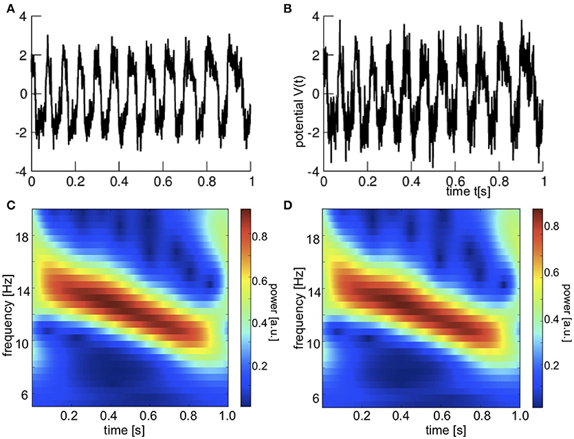
Figure 2. Noisy in-situ observations. (A) Time series for medium noise level κ = 0.5. (B) Time series for large noise level κ = 0.8. (C) Time-frequency distribution for medium noise level κ = 0.5. (D) Time-frequency distribution for large noise level κ = 0.8.
From Equation (4), one reads off the observation operator
with y = Hx, x = (V, w)t ∈ ℜ2.
For comparison, we also consider nonlocal observations with the observation operator
yielding
for the same noise levels κ as above. Figure 3A shows time series and corresponding time-frequency distributions. The frequency of the oscillation decreases over time similar to the in-situ observations.

Figure 3. Nonlocal and speed observations at various measurement noise levels κ. (A) Time series and time-frequency distributions of nonlocal observations (B) time series of speed observations.
As already stated, the aim of the present work is to introduce the idea to forecast temporal features. As a further step in this direction, let us consider temporal changes of the signal evolution, i.e., the speed of the system. To this end the definition of the observation operator is extended to
with
yielding
for two noise levels κ = 0.0 and κ = 0.02. Numerically, the derivative dV(t)/dt is implemented as V(tn) − V(tn−1) at time instance tn. Figure 3B shows the corresponding time series. We recognize the short time scale of the spike activity in in-situ observations as couples of sharp positive and negative spikes.
2.3. Ensemble Transform Kalman Filter
One of the major aims of data assimilation techniques is the optimal fit of model dynamics to observed data. Here, we introduce the major idea with a focus on the 2-dimensional model (1) and the scalar observation. Observations y(t) evolve in the 1-dimensional observation space, while the model solutions are embedded in the 2−dimensional model phase space.
2.3.1. Analysis Ensemble
To merge observation y(t) and model background state xb(t) at time t optimally, the best new model state xa minimizes the cost function
i.e., the solution is the minimum of the cost function C. Here, H is the observation operator, xa is called the analysis, B is the model error covariance matrix and R the observation error. If the assumed dynamical model and the assumed observation operator used in the data assimilation procedure are the true model and operator, respectively, then the assumed observation error is identical to the true error, i.e., R = κ2. However, typically, one does not know the true observation error κ and R can just be estimated. This is the case we consider in the present work. In the present implementation R = 1.5. For given matrix B and the scalar R, the optimal new model state is
This is the major result of the 3DVar technique for scalar observations [10].
Conversely, if the covariance error matrix B is not known, it can be estimated from the model. To this end, one considers an ensemble of model states of L ensemble members and estimates B by
with the ensemble mean and . In applications, we choose L = 10 if not stated differently. Introducing the equivalent of X in observation space Y = HX, Equation (8) reads in model space
and in observation space
with ya, b = Hxa, b. Since YYt and R are positive-definite scalars,
stating that the analysis equivalent in observation space ya is always closer to the observation as the background equivalent in observation space yb.
The ensemble transform Kalman filter (ETKF) [22] optimizes observation and background ensemble members to gain an analysis ensemble in the ensemble space. This space is L-dimensional and is spanned by the ensemble members
with the ensemble space coordinates w ∈ ℜL. Re-considering the optimization scheme (7) in this space
with and the identity matrix I ∈ ℜL×L. Then the analysis ensemble mean and its covariance Pa reads
The analysis ensemble members can be calculated by
with . Let us define the deviations from the analysis mean
corresponding to (10) and with Wl ∈ ℜL. Defining the matrix W ∈ ℜL×L with columns Wl, the ansatz P = WWt, and Equation (15) yields . With the singular value decomposition P = UDUt, the orthogonal matrix U and the diagonal matrix D, essentially we gain
where . This is the square-root filter implementation of the ETKF [23].
Equation (7) implies that all states, observations, covariances and operators are instantaneous. Extensions of this formulation are known, e.g., as the 4D-ENKF or the 4DVar [24–26]. Most of these previous extensions imply an instantaneous observation operator . In the previous section, we considered the speed of observations as the observations under study implying the temporal derivative of observed signals. This derivative is nonlocal in time and hence non-instantaneous. Here, we argue that the system evolves on a time scale that is much larger than the sampling time or, in other words, the sampling rate is high enough that the temporal derivative can be considered as being local in time. Consequently, Equation (7) may still hold in a good approximation.
2.3.2. Inflation
In each analysis step, the analysis equivalent in observation space ya moves away from the model background state yb closer to the observation y, cf. discussion of Equation (13). This assumes that observations reflect the true state. Of course, observations usually are errorneous due to measurement errors or errors in the observation operator. This is taken care of by the model error covariance matrix R. The uncertainty of the model state in observation space is described by the covariance estimator YYt. However, the model has errors which are not completely reflected by the state estimate error covariance matrix YYt, since this is calculated based on an ensemble of model forecasts with the same simulated model equations. To take care of the model error and draw the analysis closer to the background state, typically one enhances the ensemble spread by inflation.
For in situ- and nonlocal observations we have implemented constant multiplicative inflation by scaling in Equation (16) by a factor . In addition, we employed additive covariance inflation by B → B+0.15I in Equation (10) with the 2 × 2 unity matrix I. For speed observations, we have reduced the multiplicative inflation factor to 1.05 and the additive covariance inflation factor to 0.05.
2.4. Data Assimilation Cycling
Putting together models and data assimilation, the model evolution is controlled by observed data optimizing the initial state of the model iteration. Our data assimilation cycle starts with initial conditions from which the model evolves during the sampling interval. The model state after one sampling interval Δt is the background state or first guess xb. The subsequent data assimilation step estimates the analysis state xa that represents the initial state for the next model evolution step. In other words, data assimilation tunes the initial state for the model evolution after each sampling interval. Using the ETKF, this cycling is applied for all ensemble members which obey the model evolution and whose analysis state is computed in each data assimilation step. Initial ensemble member model states were with random uniformly distributed numbers η1, η2 in the range η1, η2 ∈ [0;1].
2.5. Ensemble Prediction and Verification
The aim of the present work is to show how optimal forecasting can be done. Free ensemble forecasts are model evolutions over a time typically longer than the sampling time. This forecast time is called lead time. The initial state of the free forecasts are the analysis model states determined by data assimilation.
In the present work, we are interested in forecasts at every sample time instant. To this end we compute the model activity at a certain lead time. This forecast is computed for all ensemble members what renders it an ensemble prediction. The forecasts are solutions of the model at time t≥ta with initial analysis state xa at time t = ta and lead time T = t−ta. To compare them to observations, forecasts are mapped to observation space yielding model equivalents
Later sections show free forecasts yf(t; t−T) with fixed lead time. In the following, model forecasts with the sampling time as lead time T = Δt are called first guess.
Naturally, one expects that the forecasts diverge from observations with longer lead times but the question is which forecasts can still be trusted, i.e., are realistic. Essentially we ask the question how one can verify the forecasts. To this end, various metrics and scores have been developed [27]. Since most forecasts are validated against observations, metrics are based on model forecast equivalents in the observation space.
2.5.1. First Guess Departure Statistics
To estimate the deviation of forecast ensemble members with forecast ensemble means from observations yn, n = 1, …, N of number N, we compute the mean error (bias)
the root-mean square error
and the ensemble spread
For scalar observations and corresponding forecasts, i.e., temporal time series, and N is the number of time points. Conversely, for time-frequency distributions S(t, ν) computed from the observation time series by a wavelet transform (cf. section 2.1) with K time points and M frequencies, and N = KM is the number of all time-frequency elements.
The time-frequency distribution represents the spectral power distribution S at various time instances. Since spectral power is a positive-definite measure, the distance of two time-frequency distributions could be computed differently as a root mean square error. We can interpret the rmse as the Euclidean distance in high-dimensional signal space. However, the spectral power lies on a manifold in signal space and hence the distance between spectral power values is a Riemannian distance [28, 29]. Alternatively, the distance between time-frequency distributions may represent the temporal average of distances between two instantaneous power spectra S1(tk, ν), S2(tk, ν) at time instance tk. A corresponding well-known distance measures is the time-averaged Itakura-Saito distance (ISD) [29, 30]
This distance measure is not symmetric in the spectral distributions and hence not a metric. As an alternative, one may also consider the log-spectral distance (LSD) [29, 31]
which has the advantage that it is symmetric in the distributions. In both latter measures Sobs and Sfc are the power spectra of observations and forecasts, respectively.
As pointed out above, we hypothesize that spectral features extracted from forecasts can be predicted in a better or more precise way than forecasts themselves. Since measurement noise plays an important role in experimental data, we evaluate predictions for medium and large noise levels κ compared to κ = 0. The skill score [32]
reflects the deviation of forecast errors at medium and large noise levels from noiseless forecasts. For SS = 0, forecasts have identical rmse and SS < 0 (SS > 0 ) reflects larger (smaller) rmse, i.e., worse (better) forecasts. The skill score SS is less sensitive to the bias as the rmse, and that also plays an important role in the evaluation of forecasts (similarly to the standard deviation). However, for small bias SS > 0 is a strong indication of improved forecasts.
According to Equation (10), the ensemble is supposed to describe well the model error. The ensemble spread represents the variability of the model and an optimal ensemble stipulates spread = rmse [33]. The spread-skill relation [34]
quantifies this relation. If SSR > 1, the ensemble spread is too large yielding bad estimates of the analysis ensemble and free forecasts, whereas SSR < 1 reflects a too small spread giving observations too much weight and yielding bad estimates of analysis ensemble and forecasts as well.
2.5.2. Ensemble Distribution Statistics
A representative forecast ensemble has the same distribution as the observations. This can be quantified by computing the rank of an observation in a forecast ensemble [35, 36]. If this rank is uniformly distributed, then the ensemble describes well the variability of the observations. Conversely, if the rank distribution has an U-shape (inverse U-shape) then most observations lie outside (inside) the range of the ensemble and the forecast ensemble is not representative. To estimate the shape of the rank distribution, we parameterize it by a beta-function
with the gamma-function Γ(x) and two parameters α, β > 0. For a uniform distribution α = β = 1, and U-shape (inverse U-shape) distributions have α, β < 1 (α, β > 1). Computing the sample of ranks r ∈ [0, L] from the set of forecast ensembles and observations, their mean μ and variance σ2 permits to estimate the function parameters by
The derived β−score [35]
equals 0 for a uniform distribution and βc > 0 (βc < 0) reflects the ensemble overestimation (underestimation) of the model uncertainty for an inverse U-shaped (U-shaped) distribution. In addition, the β-bias [35]
quantifies the skewness of the rank distribution and βb = 0 reflects symmetric distributions. β−bias values βb > 0 (βb < 0) reflect a weight to lower (higher) ranks and the majority of ensemble members is larger (smaller) than observations.
3. Results
At first, we consider in-situ observations and evaluate the data assimilation cycle to illustrate some properties of the ETKF. Subsequently, we present forecasts for in-situ observations as time series and time-frequency distributions and evaluate the corresponding ensemble forecasts by statistical metrics well-known from verification in meteorology. To understand the specific nature of in-situ observations, subsequently we also consider nonlocal observations and speed observations and present corresponding verification results. Eventually, we compute advanced statistical estimates specific for spectral power distributions and verify corresponding forecasts.
3.1. Data Assimilation Cycle—in-situ Observations
To start, we consider in-situ observations. Figure 4 shows observations, the ensemble mean of first guess and analysis equivalents in observations space. We observe that the analysis (red) is always closer to the observation (black) than the first guess (blue). This validates Equation (13). Moreover, visual inspection tells that higher noise levels yields worse fits of the first guess and the analysis to observation. This will be quantified in more detail in later section 3.3.
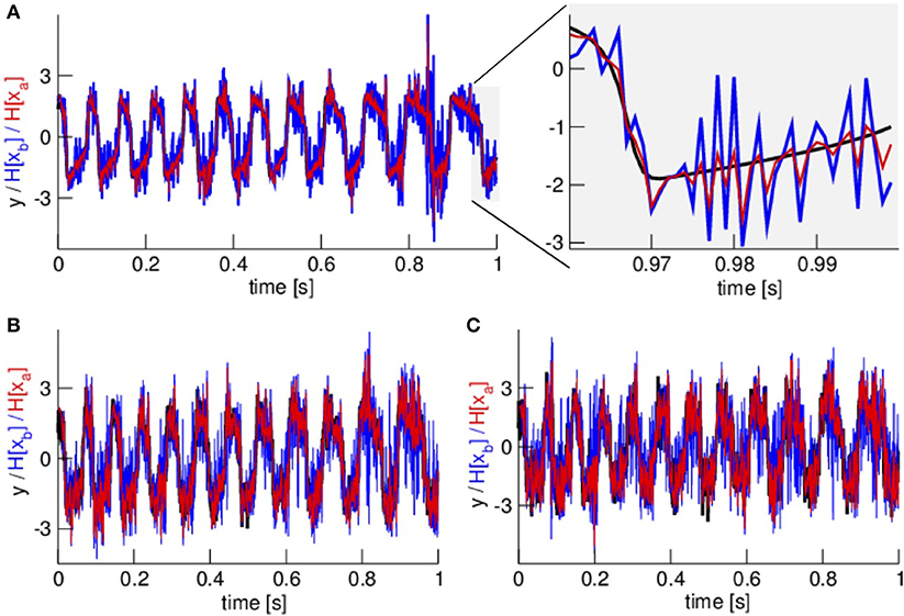
Figure 4. In-situ observations y, ensemble mean of first guess and ensemble mean of analysis in observation space for no noise κ = 0 (A), medium noise level κ = 0.5 (B), and large noise level κ = 0.8 (C). In (A) the right panel zooms in a signal part illustrating that the analysis mean (in observation space, red color) is closer to the observations (black color) than the first guess mean (in observation space, blue color) in accordance to theory, see section 2. In all panels, observations are color-coded in black, first guess equivalents in observation space in blue and analysis equivalents in observation space in red.
To illustrate the ensemble evolution, Figure 5 shows observations and the ensemble mean (blue solid line) and the single ensemble members (blue dots) of the first guess in an initial and final time interval. We observe that the ensemble starts with a narrow distribution while it diverges rapidly after several time steps. The ensemble spread about the ensemble mean reached after the initial transient phase remains rather constant over time.
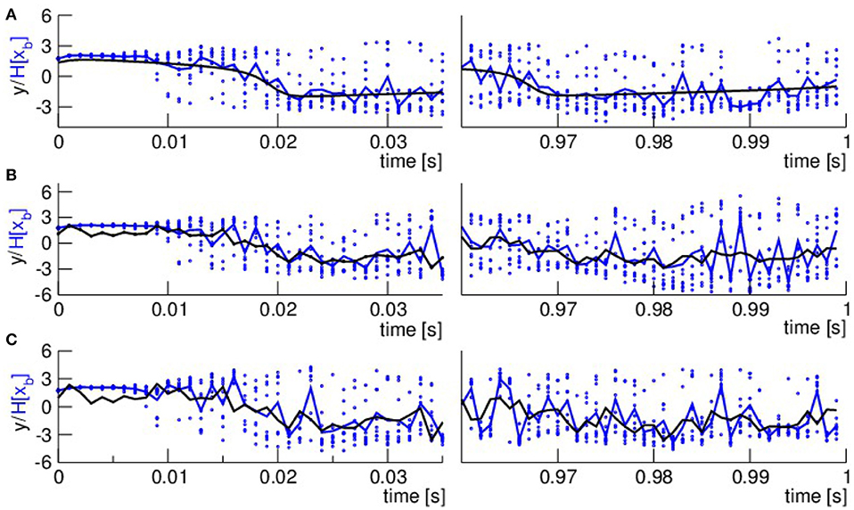
Figure 5. Illustration of the temporal evolution of ensemble spread in observation space. (A) κ = 0, (B) κ = 0.5, (C) κ = 0.8. Observations are color-coded in black, the ensemble mean of the first guess is color-coded in blue and solid line and the single ensemble members are color-coded in blue and single dots.
3.2. Forecast—in-situ Observations
Now let us turn to the forecasts. In the data assimilation cycle, after one model step and hence one sampling time interval, the analysis is computed and initializes the phase space trajectory of the model evolution for the subsequent model step. In free forecasts , the model is integrated over a certain lead time T = t−ta initialized by the analysis at each time instant ta. Figures 6A–C shows time series of observations and forecast ensemble mean equivalents for two lead times. For the short lead time T = 10 ms the first guess equivalent follows rather closely the observation, whereas it is phase-shifted to the observation for large lead time 40 ms. This holds true for all noise levels.
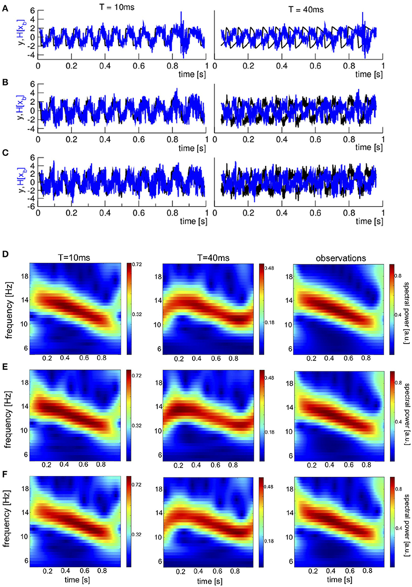
Figure 6. In-situ time series and time-frequency distributions of free ensemble forecasts for two lead times T and different noise levels. (A–C) Time series, observations are color-coded in black, the ensemble mean of first guess equivalents in observation space is color-coded in blue. (D–F) Time-frequency distributions. The forecasts shown are ensemble means of first guess equivalents in observation space . It is important to re-call that disturbances occur in a window of 4/f from the left and right temporal borders where f is the corresponding frequency, cf. section 2. (A,D) κ = 0, (B,E) κ = 0.5, and (C,F) κ = 0.8.
The time-frequency distribution of the observations and forecast equivalents is shown in Figures 6D–F. The time-frequency distribution of forecasts at short lead time resembles well the time-frequency distribution of observations, whereas prominent differences between large lead time-forecasts and observations occur, especially at the temporal borders.
3.3. Verification—in-situ Observations
To quantify the differences between forecasts and observations detected by visual inspection in section 3.2, we compute the forecast departure statistics subject to the lead time. Figure 7A shows that rmse of time-frequency data increases monotonically with lead time and it increases and finally decreases when based on time series data. The periodicity of rmse results from the increasing forecast-observation delay that increases with the lead time. Hence at a phase lag of π when the lead time is half the mean oscillation period the rmse is maximum. This explains why the two rmse minima have a temporal distance of ~70 ms what corresponds to one period of the mean system frequency of 14 Hz. Moreover, the bias decreases monotonically with the lead time for time series and increases for time-frequency data. To summarize these findings, we compute the skill score SS. Since the rmse for different noise levels approach each other for large lead times the skill score approaches SS = 0 (Figure 7B]. We observe that the skill score of time-frequency data exceeds SS of time series data.
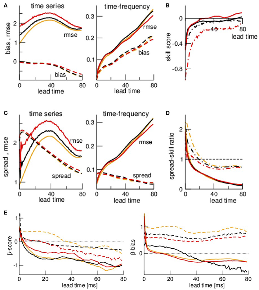
Figure 7. Ensemble verification metrices and scores with respect to lead times. (A) rmse (solid line) and bias (dashed line) based on time series and time-frequency distributions. (B) Skill score SS(κ) = 1−rmse(κ)/rmse(0). (C) rmse (solid line) and spread (dashed line) based on time series and time-frequency distributions. (D) Spread-skill ratio SSR = spread/rmse. (E) Features of ensemble rank histogram β-score and β-bias with respect to lead times. Colors in (A,C,D,E) encode κ = 0 (orange), κ = 0.5 (black), and κ = 0.8 (red), line types in (B,D,E) encode time series data (dashed-dotted) and time-frequency distributions (solid). The estimates bias, rmse, and spread are averages over N = 1, 000 observations for each lead time.
The ensemble spread decreases with lead time in both time series data and time-frequency data to values smaller than the rmse. This yields a decreasing spread-skill relation where SSR is well below SSR = 1 for both time series data and time-frequency distribution data. We note that SSR falls faster to lower values for time-frequency distribution data. Since one expects of good filters that the ensemble variations (spread) explain well the error (rmse), here the forecast ensemble of time series explains better the observations than time-frequency data since their SSR is closer to SSR = 1.
The reliability of the ensemble forecasts can be evaluated by rank histograms, i.e., the β−score βc and β−bias βb. Figure 7E shows that βc decreases from positive to negative values both for time series and time-frequency distribution data. This reveals an underestimation of the model uncertainty. The β−bias remains positive-definite for time series data whereas βb of time-frequency distribution data decreases from positive to negative values. This result reveals that the majority of ensemble members are larger than the time series observations and smaller than the time-frequency spectral power observations.
To understand better why the ensemble spread shrinks at large lead time, Figure 8 compares the ensemble mean of the model forecasts in phase space with the true phase space data. The forecasts exceed the true data at lead time T = 1 ms. Conversely the forecast spread is much smaller than the true data at T = 80 ms since the forecasts obey the false model dynamics that evolves on a smaller phase space regime. Consequently the spread shrinkage with the lead time results from the smaller phase space regime of the false model.
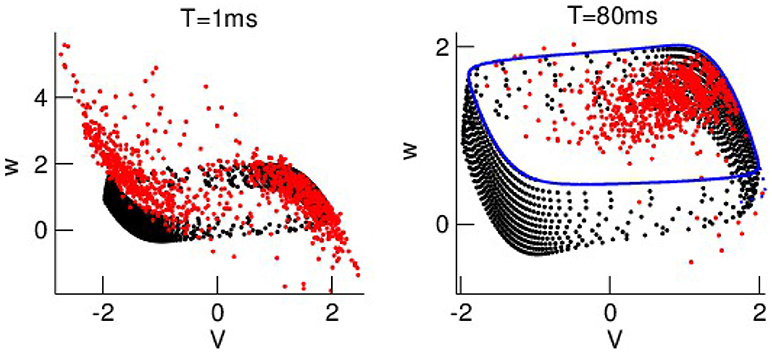
Figure 8. Phase space dynamics for short and long lead times. The ensemble mean of forecasts and the true data are color-coded in red and black, respectively. The blue-coded points represent the false model data.
3.4. Nonlocal Observations
To understand how specific the gained results from in-situ observations are, we compare them to statistics of other data type. Now let us consider nonlocal observations subjected to various noise levels. Figures 9B–D shows the time-frequency distributions for three noise levels and three lead times T. Forecasts at medium lead time T differ clearly to observations and forecasts at short and long lead time.
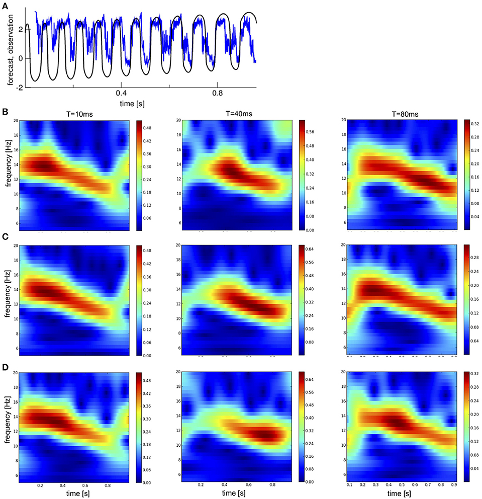
Figure 9. Time series and time-frequency distributions of free ensemble mean forecasts compared to nonlocal observations. (A) Forecast for T = 40ms (blue) and noise-free observations (black). (B–D) Forecasts for two lead times T and observations at different noise levels. (B) κ = 0, (C) κ = 0.5, and (D) κ = 0.8.
To understand this, we take a closer look at the forecast time series at T = 40 and compare it to the observations, cf. Figure 9A. Re-call that the analysis sets the initial condition for forecasts. For a lead time T = 40 ms the forecasts are in a fixed phase relation to an observation oscillations with ν0 = 12.5 Hz since then T = 1/ν0 is exactly one period of this oscillation. This fixed phase relation is observed in Figure 9A at ~0.5 s. Before and after that time, the observation frequency is larger and smaller, respectively, see also Figure 6, and the forecasts are out of phase. In addition, in the beginning and end the forecasts do not evolve rhythmically yielding missing spectral power, cf. Figures 9B–D. Summarizing, forecasts may resonate with oscillatory observations at frequency ν0 = 1/T.
The departure statistics between forecasts and observations resembles the findings for in-situ observations, cf. Figure 10A. Time-frequency distributions have almost optimal skill score SS for medium and large lead times, however with too small ensemble spread (SSR is very small). Conversely, time series data yield worse skill score but larger ensemble spread. Moreover, the rmse and bias have a maximum at about T = 25 ms and a minimum at about T = 45 ms. The minimum is explained above as a resonance between forecast time and observation frequency.
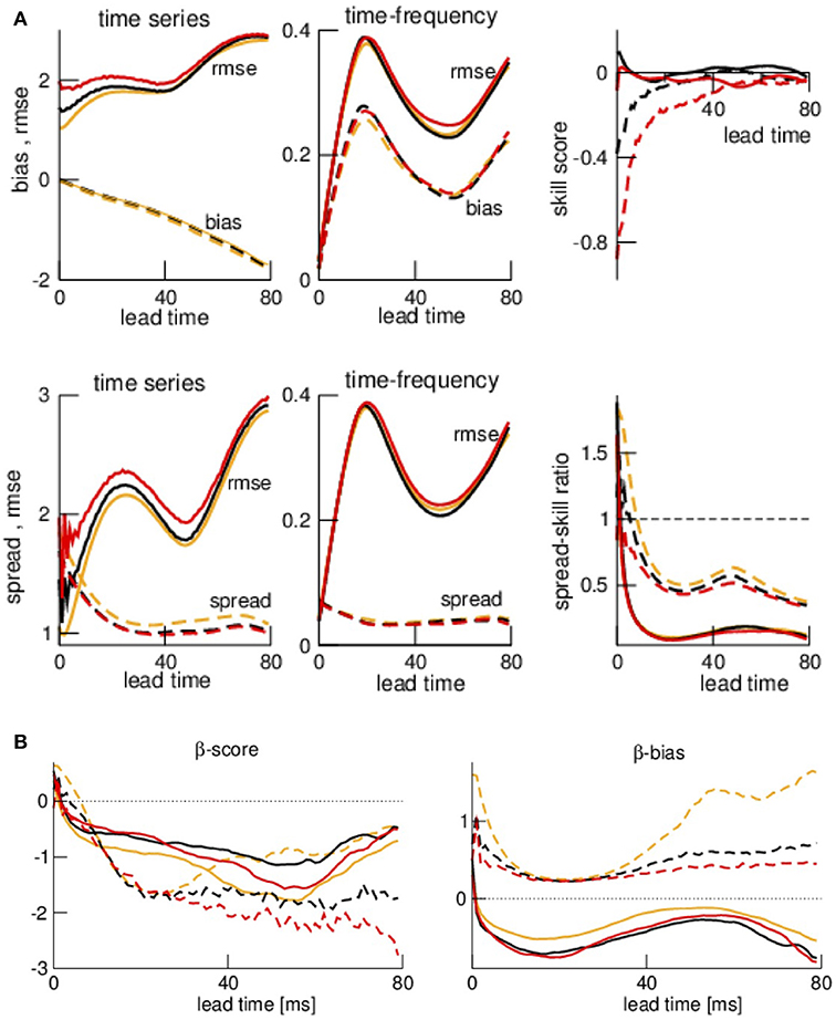
Figure 10. The departure metrics Bias, rmse and spread of forecasts of nonlocal observations, the corresponding skill score SS and spread-skill ratio SSR (A) and the rank statistics βc and βb (B). The color- and line-coding is identical to the Figure 7. The estimates Bias, rmse, and spread are averages over N = 1, 000 observations for each lead time.
These results are in good accordance to the rank histogram features βc and βb seen in Figure 10B. Very short lead times yield βc > 0 reflecting an overestimation of the spread, otherwise βc < 0 reflecting a too small ensemble spread. This holds true for all data types and all noise levels. The β−bias is similar to Figure 7 and shows that the majority of the ensemble members is larger than the time series observations and smaller than the spectral power values.
Summarizing, the ensemble varies much with the lead time what indicates a fundamental problem in the ensemble forecast.
3.5. Speed Observations
Spectral power takes into account data at several time instances. Since to our knowledge Kalman filters have not been developed yet for observation operators nonlocal in time, we take a first step and consider speed observations subjected to two noise levels. Figure 11A compares observations, first guess and analysis in data assimilation cycling for the same number of ensemble members as in the previous assimilation examples. We observe that the first guess and analysis do not fit at all to the observations and hence the assimilation performs badly.
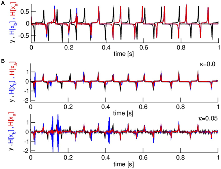
Figure 11. Observations, first guess and analysis for speed data. (A) Noise-free observations and low number of ensemble members L = 10. (B) Two measurement noise levels and the modified assimilation parameters R = 0.01, L = 50, and the modified inflation factors.
To improve the assimilation cycle, we diminish the observation error to R = 0.01 drawing the analysis closer to the observations. In addition, a larger ensemble improves the estimation of the model covariance inflation and we increase the number of ensemble members to L = 50 while decreasing the inflation factors to 1.05 (multiplicative inflation) and 0.05 (additive inflation). Figure 11B demonstrates that these modifications well improve the assimilation cycle. Now the first guess and analysis fit much better to the observations. An increased noise level renders the first guess and analysis less accurate.
The forecasts in Figure 12 show that the assimilation cycle captures the upper observation spikes for T = 40 ms whereas forecasts at larger lead times are worse.
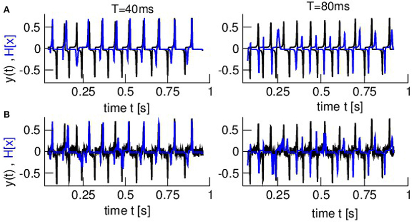
Figure 12. Time series of observations and forecasts (model equivalent in observation space) at two lead times and two noise levels. (A) κ = 0.0 (B) κ = 0.05. Observations are color-coded in black and forecasts in blue. Parameters are identical to parameters in Figure 11.
This can be quantified by departure statistics metrics as shown in Figure 13. The rmse increases slightly with lead time, i.e., the forecast error is larger for larger forecast times, while the bias is rather lead-time independent. Moreover, we observe that the spread is much smaller than the rmse. Since reliable ensemble forecasts should have a unity spread-skill ratio, this too small spread reflects a too small analysis inflation factor.
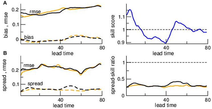
Figure 13. The departure metrics bias, rmse, and spread of forecasts to speed observations and the corresponding skill score SS and spread-skill ratio SSR. Comparison of (A) bias and rmse and (B) spread and rmse. The skill score relates the rmse at both noise levels. The colors encode the noise level κ = 0 (orange) and κ = 0.05 (black). Parameters are identical to parameters in Figure 11.
These results are in good accordance to the rank histogram features βc and βb seen in Figure 14. The negative values of βc for all lead times reflects the underestimation of the spread and the β−bias βb≈0 indicates that this underestimation is present for all forecast values. This holds true for both noise levels.
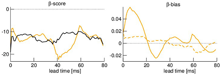
Figure 14. Rank statistics βc and βb for the ensemble in the presence of speed observations. The color-coding is identical to Figure 13. Parameters are identical to parameters in Figure 11.
3.6. Advanced Statistical Measures
Since the rmse is not an optimal measure to quantify the difference between time-frequency distributions, we compute more advanced measures specific for power spectra. The Itakura-Saito distance (ISD) and the log-spectral distance (LSD) increase with the lead time for in-situ observations with a light local maximum at about T = 40 ms, cf. Figure 15A. A closer look at Figure 6 reveals that the forecast spectral power at T = 40 is much smaller than the observation spectral power explaining this local increase of distance. The time-frequency distribution distances are rather similar in all noise levels. Moreover, spectral distances between nonlocal observations and forecasts exhibit a strongly non-monotonic dependence of the lead time. This is in good accordance to the results with the rmse in Figure 10.

Figure 15. Improved verification statistics of in-situ and non-local observations. (A) Itakura-Saito distance (ISD) and log-spectral distance (LSD) between forecasts and in-situ observations (left panel) and between forecasts and non-local observations (right panel) at various lead times. The distance measures are averages over the full time interval. (B) rmse, Itakura-Saito distance (ISD), and log-spectral distance (LSD). Here, the distance measures are averages over the constraint time interval [0.3s; 0.7s] to take care of the border effects generated the wavelet transform.
Time frequency distributions appear to represent instantaneous spectral power. However, the spectral power distributions at subsequent time instances are strongly correlated dependent on the frequency. The correlation length is τ = 4/f leading to distortions at the temporal borders. Since the major spectral power occurs in the frequency interval [11 Hz;15 Hz], i.e., for correlation times 0.27 ≤ τ ≤ 0.36, we define distorted time intervals with width 0.3 s and estimate improved time-frequency distribution distances neglecting the distorted initial and final time interval. Figure 15B shows the corresponding results. We observe that rmse, ISD and LSD depend similarly on the lead time for both data types. Moreover, ISD and LSD are slightly smaller than their equivalents for the full time interval shown in Figure 15A.
4. Discussion
The present work applies well-established techniques known in meteorology to find out whether they can be useful to forecast spectral features in other science domains where spectral dynamics plays an important role, such as in neuroscience. For in situ- and nonlocal observations, the assimilation of spectral features is indirect since the features are computed after the computation of conventional forecasts, i.e., in time series. We show that they strongly improve skill scores (Figures 7, 10] for large lead times, whereas their spread is worse than for conventional forecasts for large lead times. This holds true for all measurement noise levels under study. In general, the ensemble forecast verification points to problems with the ensemble spread in all data types. This may result from a poor estimation of the model error covariance B by too few ensemble members and a non-optimal choice of the inflation factor.
Since time-frequency distributions show time-variant spectral power, it is necessary to verify forecasts by spectral power-specific measures and take care of spectral power-specific artifacts, cf. Figure 15. The conventional estimate rmse and the spectral-power specific estimates ISD and LSD behave similarly with respect to the lead time. Small differences between rmse and both ISD and LSD originates from the fact that ISD and LSD are time-averages over instantaneous spectral distance measures, whereas rmse averages over all frequencies and time instances and hence smoothes differences. Consequently ISD and LSD appear to be better verification measures of time-frequency distributions. Since LSD is a metric but ISD is not, future work will derive score measures based on LSD equivalent to the skill score SS. Moreover, we find that the border artifacts introduced by the wavelet transform do not affect our results qualitatively. Nevertheless, we recommend to exclude these artifacts in future work.
Conversely, speed observations consider the dynamical evolution of the system and are a very first approximation to a direct spectral feature. This is true since speed observations do not take into account the system state and observation at a single time instance only. Future work will extend this approach to a larger time window what allows to compute the power spectrum that can be mapped to a single time instance. Since generalizations or differential operators are integral operators [37], future work will consider integral observation operators.
Since spectral feature forecasts are sensitive to certain frequencies, they are sensitive to lead time-observation frequency resonances. Such resonances seem to improve the forecast although these resonances are artifacts. To our best knowledge, the current work is the first to uncover these resonances that may play an important role in the interpretation of forecasts.
The ensemble data assimilation cycle involves several modern techniques, such as multiplicative and additive covariance inflation that well improves the forecasts. As a disadvantage, the spread for short lead times is too large. Future work will improve the ensemble statistics by adaptive inflation factors [38] and quality control methods, e.g., first guess checks [39] to remove outliers in every data assimilation step. This will surely contribute to improve ensemble forecasts.
The ensemble Kalman filter applied is one possible technique to gain forecasts. Other modern powerful techniques are the variational methods 3D- and 4D-Var [40], hybrids of ensemble and variational techniques like the EnVar [41] and particle filters [42, 43]. These techniques have been applied successfully in meteorological services world-wide and future work will investigate their performance in forecasting of power spectra.
Eventually, the present study considers a specific model system that exhibits a single time scale due to a single oscillation frequency. However, natural complex systems exhibit multiple time scales what may render the Kalman filter less effective and the superiority of the time-frequency data less obvious. In the future, it will be an important task to extend the present work to multi-scale Kalman filters [44, 45].
Author Contributions
AH conceived the study and performed all simulations. AH and RP planned the manuscript structure and have written the manuscript.
Conflict of Interest Statement
The authors declare that the research was conducted in the absence of any commercial or financial relationships that could be construed as a potential conflict of interest.
Acknowledgments
The authors would like to thank Felix Fundel, Michael Denhardt, and Andreas Rhodin for valuable discussions.
References
2. Schiff S, Sauer T. Kalman filter control of a model of spatiotemporal cortical dynamics. J Neural Eng. (2008) 5:1–8. doi: 10.1088/1741-2560/5/1/001
4. Kalnay E. Atmospheric Modeling, Data Assimilation and Predictability. Cambridge, UK: Academic Press (2002).
5. Assi E, Nguyen D, Rihana S, Sawan M. Towards accurate prediction of epileptic seizures: a review. Biomed Sign Proc Control (2017) 34:144–57. doi: 10.1016/j.bspc.2017.02.001
6. Park Y, Luo L, Parhi K, Netoff T. Seizure prediction with spectral power of EEG using cost-sensitive support vector machines. Epilepsia (2011) 52:1761–70. doi: 10.1111/j.1528-1167.2011.03138.x
7. Chisci L, Mavino A, Perferi G, Sciandrone M, Anile C, Colicchio G, et al. Real-time epileptic seizure prediction using AR models and support vector machines. IEEE Trans Biomed Eng. (2010) 57:1124–32. doi: 10.1109/TBME.2009.2038990
8. Ullah G, Schiff S. Assimilating seizure dynamics. PLoS Comput Biol. (2010) 6:e1000776. doi: 10.1371/journal.pcbi.1000776
9. Sedigh-Sarvestani M, Schiff S, Gluckman B. Reconstructing mammalian sleep dynamics with data assimilation. PLoS Comput Biol. (2012) 8:e1002788. doi: 10.1371/journal.pcbi.1002788
10. Nakamura G, Potthast R. Inverse Modeling - An Introduction to the Theory and Methods of Inverse Problems and Data Assimilation. Bristol, UK: IOP Publishing (2015).
11. Alswaihli J, Potthast R, Bojak I, Saddy D, Hutt A. Kernel reconstruction for delayed neural field equations. J Math Neurosci. (2018) 8:3. doi: 10.1186/s13408-018-0058-8
12. Hashemi M, Hutt A, Buhry L, Sleigh J. Optimal model parameter estimation from EEG power spectrum features observed during general anesthesia. Neuroinformatics (2018) 16:231–51. doi: 10.1007/s12021-018-9369-x
13. Fries P. Neuronal gamma-band synchronization as a fundamental process in cortical computation. Annu Rev Neurosci. (2009) 32:209–24. doi: 10.1146/annurev.neuro.051508.135603
14. Hutt A (ed.). Sleep and Anesthesia: Neural Correlates in Theory and Experiment. No. 15 in Springer Series in Computational Neuroscience. New York, NY: Springer (2011).
15. Roth M, Hendeby G, Fritsche C, Gustafsson F. The Ensemble Kalman Filter: a signal processing perspective. EURASIP J Adv Sign Process. (2017) 2017:56. doi: 10.1186/s13634-017-0492-x
17. Roth M, Fritsche C, Hendeby G, Gustafsson F. The Ensemble Kalman Filter and its relations to other nonlinear filters. In: Proceedings of the 2015 European Signal Processing Conference (EUSIPCO 2015), Institute of Electrical and Electronics Engineers (IEEE) (New York, NY) (2015). p. 1236–40.
18. FitzHugh R. Mathematical models of threshold phenomena in the nerve membrane. Bull Math Biophys. (1955) 17:257–78.
19. Nagumo J, Arimoto S, Yoshizawa S. An active pulse transmission line simulating nerve axon. Proc IRE (1962) 50:2061–270.
20. Hutt A, Lefebvre J, Hight D, Sleigh J Suppression of underlying neuronal fluctuations mediates EEG slowing during general anaesthesia. Neuroimage (2018) 179:414–28. doi: 10.1016/j.neuroimage.2018.06.043
21. Hashemi M, Hutt A, Sleigh J How the cortico-thalamic feedback affects the EEG power spectrum over frontal and occipital regions during propofol-induced anesthetic sedation. J Comput Neurosci. (2015) 39:155–79. doi: 10.1007/s10827-015-0569-1
22. Hunt B, Kostelich E, Szunyoghc I. Efficient data assimilation for spatiotemporal chaos: a local ensemble transform Kalman filter. Phys D (2007) 230:112–26. doi: 10.1016/j.physd.2006.11.008
23. Tippett M, Anderson J, Bishop C, Hamill T, Whitaker J. Ensemble square root filters. Mon Weather Rev. (2003) 131:1485–90. doi: 10.1175/1520-0493(2003)131<1485:ESRF>2.0.CO;2
24. Fertig E, Harlim J, Hunt B. A comparative study of 4D-Var and a 4D ensemble kalman filter: perfect model simulations with Lorenz-96. Tellus (2007) 59A:96–100. doi: 10.1111/j.1600-0870.2006.00205.x
25. Le Dimet F, Talagrand O. Variational algorithm for analysis and assimilation of meteorological observations: theoretical aspects. Tellus (1986) 38A:97–110.
26. Hunt B, Kalnay E, Ott E, Patil D, Sauer T, Szunyogh I, et al. Four-dimensional ensemble kalman filtering. Tellus (2004) 56A:273–7. doi: 10.3402/tellusa.v56i4.14424
27. Mason S. Understanding forecast verification statistics. Meteorol Appl. (2008) 15:13040. doi: 10.1002/met.51
28. Li Y, Wong KM. Riemannian distances for signal classification by power spectral density. IEEE J Select T Sign Proc. (2013) 7:655–69. doi: 10.1109/JSTSP.2013.2260320
29. Jiang X, Ning L Georgiou TT Distances and Riemannian metrics for multivariate spectral densities. IEEE Trans Auto Contr. (2012) 57:1723–35. doi: 10.1109/TAC.2012.2183171
30. Iser B, Schmidt G, Minker W. Bandwidth Extension of Speech Signals. Heidelberg: Springer (2008).
31. Rabiner L, Juang B. Fundamentals of Speech Recognition. Upper Saddle River, NJ: PTR Prentice Hall (1993).
32. Murphy AH Skill scores based on the mean square error and their relationships to the correlation coefficient. Monthly Weather Rev. (1988) 116:2417–24.
33. Weigel A. Ensemble verification. In: Joliffe I, Stephenson D, editors. Forecast Verification: A Practitioner's Guide in Atmospheric Science. 2nd Edn. Chichester: John Wiley and Sons (2011). p. 141–66.
34. Hopson T. Assessing the ensemble spread-error relationship. Mon Weather Rev. (2014) 142:1125–42. doi: 10.1175/MWR-D-12-00111.1
35. Keller J, Hense A. A new non-Gaussian evaluation method for ensemble forecasts based on analysis rank histograms. Meteorol Zeitsch. (2011) 20:107–17. doi: 10.1127/0941-2948/2011/0217
36. Hamil T. Interpretation of rank histograms for verifying ensemble forecasts. Mon Weather Rev. (2000) 129:550–60. doi: 10.1175/1520-0493(2001)129<0550:IORHFV>2.0.CO;2
37. Hutt A. Generalization of the reaction-diffusion, Swift-Hohenberg, and Kuramoto-Sivashinsky equations and effects of finite propagation speeds. Phys Rev E (2007) 75:026214. doi: 10.1103/PhysRevE.75.026214
38. Anderson J. An adaptive covariance inflation error correction algorithm for ensemble filters. Tellus (2007) 59A:210–24. doi: 10.1111/j.1600-0870.2006.00216.x
39. Geer A, Bauer P. Observation errors in all-sky data assimilation. Q J R Meteorol Soc. (2011) 137:2024–37. doi: 10.1002/qj.830
40. Gauthier P, Tanguay M, Laroche S, Pellerin S, Morneau J. Extension of 3DVar to 4DVar: implementation of 4DVar at the Meteorological Service of Canada. Monthly Weather Rev. (2007) 135:2339–54. doi: 10.1175/MWR3394.1
41. Bannister RN. A review of operational methods of variational and ensemble-variational data assimilation. Q J R Meteorol Soc. (2017) 143:607–33. doi: 10.1002/qj.2982
42. van Leeuwen P.J. Particle filtering in geophysical systems. Monthly Weather Rev. (2009) 137:4098–114. doi: 10.1175/2009MWR2835.1
43. Potthast R, Walter A, Rhodin A. A localised adaptive particle filter within an operational NWP Framework. (2018). Monthly Weather Rev. doi: 10.1175/MWR-D-18-0028.1. [Epub ahead of print].
44. Hickmann KS, Godinez HC. A multiresolution ensemble Kalman filter using the wavelet decomposition. arXiv:1511.01935 (2017).
Keywords: Kalman filter, neural activity, prediction, dynamical system, verification
Citation: Hutt A and Potthast R (2018) Forecast of Spectral Features by Ensemble Data Assimilation. Front. Appl. Math. Stat. 4:52. doi: 10.3389/fams.2018.00052
Received: 10 April 2018; Accepted: 15 October 2018;
Published: 01 November 2018.
Edited by:
Ulrich Parlitz, Max-Planck-Institut für Dynamik und Selbstorganisation, GermanyReviewed by:
Hiromichi Suetani, Oita University, JapanXin Tong, National University of Singapore, Singapore
Copyright © 2018 Hutt and Potthast. This is an open-access article distributed under the terms of the Creative Commons Attribution License (CC BY). The use, distribution or reproduction in other forums is permitted, provided the original author(s) and the copyright owner(s) are credited and that the original publication in this journal is cited, in accordance with accepted academic practice. No use, distribution or reproduction is permitted which does not comply with these terms.
*Correspondence: Axel Hutt, YXhlbC5odXR0QGR3ZC5kZQ==