CUR Decompositions, Similarity Matrices, and Subspace Clustering

1. Introduction

We present here two tales: one about the so-called CUR decomposition (or sometimes skeleton decomposition), and another about the subspace clustering problem. It turns out that there is a strong connection between the two subjects in that the CUR decomposition provides a general framework for the similarity matrix methods used to solve the subspace clustering problem, while also giving a natural link between these methods and other minimization problems related to subspace clustering.

The CUR decomposition is remarkable in its simplicity as well as its beauty: one can decompose a given matrix A into the product of three matrices, A = CU^†R, where C is a subset of columns of A, R is a subset of rows of A, and U is their intersection (see Theorem 1 for a precise statement). The primary uses of the CUR decomposition to date are in the field of scientific computing. In particular, it has been used as a low-rank approximation method that is more faithful to the data structure than other factorizations [1, 2], an approximation to the singular value decomposition [3–5], and also has provided efficient algorithms to compute with and store massive matrices in memory. In the sequel, it will be shown that this decomposition is the source of some well-known methods for solving the subspace clustering problem, while also adding the construction of many similarity matrices based on the data.

The subspace clustering problem may be stated as follows: suppose that some collected data vectors in 𝕂^m (with m large, and 𝕂 being either ℝ or ℂ) comes from a union of linear subspaces (typically low-dimensional) of 𝕂^m, which will be denoted by ${U}={\displaystyle \underset{i=1}{\bigcup ^M}}{S}_i$. However, one does not know a priori what the subspaces are, or even how many of them there are. Consequently, one desires to determine the number of subspaces represented by the data, the dimension of each subspace, a basis for each subspace, and finally to cluster the data: the data ${\left\{w_j\right\}}_{j=1}^n\subset {U}$ are not ordered in any particular way, and so clustering the data means to determine which data belong to the same subspace.

There are indeed physical systems which fit into the model just described. Two particular examples are motion tracking and facial recognition. For example, the Yale Face Database B [6] contains images of faces, each taken with 64 different illumination patterns. Given a particular subject i, there are 64 images of their face illuminated differently, and each image represents a vector lying approximately in a low-dimensional linear subspace, S_i, of the higher dimensional space ℝ^{307, 200} (based on the size of the grayscale images). It has been experimentally shown that images of a given subject approximately lie in a subspace S_i having dimension 9 [7]. Consequently, a data matrix obtained from facial images under different illuminations has columns which lie in the union of low-dimensional subspaces, and one would desire an algorithm which can sort, or cluster, the data, thus recognizing which faces are the same.

There are many avenues of attack to the subspace clustering problem, including iterative and statistical methods [8–15], algebraic methods [16–18], sparsity methods [19–22], minimization problem methods inspired by compressed sensing [22, 23], and methods based on spectral clustering [20, 21, 24–29]. For a thorough, though now incomplete, survey on the spectral clustering problem, the reader is invited to consult [30].

Some of the methods mentioned above begin by finding a similarity matrix for a given set of data, i.e. a square matrix whose entries are nonzero precisely when the corresponding data vectors lie in the same subspace, S_i, of ${U}$ (see Definition 3 for the precise definition). The present article is concerned with a certain matrix factorization method—the CUR decomposition—which provides a quite general framework for finding a similarity matrix for data that fits the subspace model above. It will be demonstrated that the CUR decomposition indeed produces many similarity matrices for subspace data. Moreover, this decomposition provides a bridge between matrix factorization methods and the minimization problem methods such as Low-Rank Representation [22, 23].

1.1. Paper Contributions

• In this work, we show that the CUR decomposition gives rise to similarity matrices for clustering data that comes from a union of independent subspaces. Specifically, given the data matrix $\text{W}=\left[w_1\cdots w_n\right]\subset {𝕂}^m$ drawn from a union ${U}={\bigcup }_{i=1}^M{S}_i$ of independent subspaces ${\left\{S_i\right\}}_{i=1}^M$ of dimensions ${\left\{d_i\right\}}_{i=1}^M$, any CUR decomposition W = CU^†R can be used to construct a similarity matrix for W. In particular, if Y = U^†R and Q is the element-wise binary or absolute value version of Y*Y, then ${\Xi }_{\text{W}}=Q^{d_{max}}$ is a similarity matrix for W; i.e., Ξ_W(i, j)≠0 if the columns w_i and w_j of W come from the same subspace, and Ξ_W(i, j) = 0 if the columns w_i and w_j of W come from different subspaces.

• This paper extends our previous framework for finding similarity matrices for clustering data that comes from the union of independent subspaces. In Aldroubi et al. [31], we showed that any factorization W = BP, where the columns of B come from ${U}$ and form a basis for the column space of W, can be used to produce a similarity matrix Ξ_W. This work shows that we do not need to limit the factorization of W to bases, but may extend it to frames, thus allowing for more flexibility.

• Starting from the CUR decomposition framework, we demonstrate that some well-known methods utilized in subspace clustering follow as special cases, or are tied directly to the CUR decomposition; these methods include the Shape Interaction Matrix [32, 33] and Low-Rank Representation [22, 23].

• A proto-algorithm is presented which modifies the similarity matrix construction mentioned above to allow clustering of noisy subspace data. Experiments are then conducted on synthetic and real data (specifically, the Hopkins155 motion dataset) to justify the proposed theoretical framework. It is demonstrated that using an average of several CUR decompositions to find similarity matrices for a data matrix W outperforms many known methods in the literature while being computationally fast.

• A clustering algorithm based on the methodology of the Robust Shape Interaction Matrix of Ji et al. [33] is also considered, and using our CUR decomposition framework together with their algorithm yields the best performance to date for clustering the Hopkins155 motion dataset.

1.2. Layout

The rest of the paper develops as follows: a brief section on preliminaries is followed by the statement and discussion of the most general exact CUR decomposition. Section 4 contains the statements of the main results of the paper, while section 5 contains the relation of the general framework that CUR gives for solving the subspace clustering problem. The proofs of the main theorems are enumerated in section 6 followed by our algorithm and numerical experiments in section 7, whereupon the paper concludes with some discussion of future work.

2. Preliminaries

2.1. Definitions and Basic Facts

Throughout the sequel, 𝕂 will refer to either the real or complex field (ℝ or ℂ, respectively). For A ∈ 𝕂^m×n, its Moore–Penrose psuedoinverse is the unique matrix A^† ∈ 𝕂^n×m which satisfies the following conditions:

1) AA^†A = A,

2) A^†AA^† = A^†,

3) (AA^†)* = AA^†, and

4) (A^†A)* = A^†A.

Additionally, if A = UΣV* is the Singular Value Decomposition of A, then A^† = VΣ^†U*, where the pseudoinverse of the m×n matrix Σ = diag(σ₁, …, σ_r, 0, …, 0) is the n×m matrix ${\Sigma }^{†}=\mathrm{\text{diag}}(1/{\sigma }_1,\dots ,1/{\sigma }_r,0\dots ,0)$. For these and related notions, see section 5 of Golub and Van Loan [34].

Also of utility to our analysis is that a rank r matrix has a so-called skinny SVD of the form $A=U_r{\Sigma }_r{V}_r^{*}$, where U_r comprises the first r left singular vectors of A, V_r comprises the first r right singular vectors, and ${\Sigma }_r=\mathrm{\text{diag}}({\sigma }_1,\dots ,{\sigma }_r)\in K^{r\times r}$. Note that in the case that rank(A) > r, the skinny SVD is simply a low-rank approximation of A.

Definition 1 (Independent Subspaces). Non-trivial subspaces ${\left\{S_i\subset K^m\right\}}_{i=1}^M$ are called independent if their dimensions satisfy the following relationship:

$dim(S_1+\cdots +S_M)=dim(S_1)+\cdots +dim(S_M)\le m.$

The definition above is equivalent to the property that any set of non-zero vectors {w₁, ⋯ , w_M} such that w_i ∈ S_i, i = 1, …, M is linearly independent.

Definition 2 (Generic Data). Let S be a linear subspace of 𝕂^m with dimension d. A set of data W drawn from S is said to be generic if (i) |W| > d, and (ii) every d vectors from W form a basis for S.

Note this definition is equivalent to the frame-theoretic description that the columns of W are a frame for S with spark d+1 (see [35, 36]). It is also sometimes said that the data W is in general position.

Definition 3 (Similarity Matrix). Suppose $\text{W}=\left[w_1\cdots w_n\right]\subset K^m$ has columns drawn from a union of subspaces ${U}={\bigcup }_{i=1}^M{S}_i$. We say Ξ_W is a similarity matrix for W if and only if (i) Ξ_W is symmetric, and (ii) Ξ_W(i, j) ≠ 0 if and only if w_i and w_j come from the same subspace.

Finally, if A ∈ 𝕂^m×n, we define its absolute value version via abs(A)(i, j) = |A(i, j)|, and its binary version via bin(A)(i, j) = 1 if A(i, j) ≠ 0 and bin(A)(i, j) = 0 if A(i, j) = 0.

2.2. Assumptions

In the rest of what follows, we will assume that ${U}={\bigcup }_{i=1}^M{S}_i$ is a nonlinear set consisting of the union of non-trivial, independent, linear subspaces ${\left\{S_i\right\}}_{i=1}^M$ of 𝕂^m, with corresponding dimensions ${\left\{d_i\right\}}_{i=1}^M$, with $d_{max}:=\underset{1\le i\le M}{max}{d}_i$. We will assume that the data matrix $\text{W}=\left[w_1\cdots w_n\right]\in {𝕂}^{m\times n}$ has column vectors that are drawn from ${U}$, and that the data drawn from each subspace S_i is generic for that subspace.

3. CUR Decomposition

Our first tale is the remarkable CUR matrix decomposition, also known as the skeleton decomposition [37, 38] whose proof can be obtained by basic linear algebra.

Theorem 1. Suppose A ∈ 𝕂^m×n has rank r. Let I⊂{1, …, m}, J⊂{1, …, n} with |I| = s and |J| = k, and let C be the m×k matrix whose columns are the columns of A indexed by J. Let R be the s×n matrix whose rows are the rows of A indexed by I. Let U be the s×k sub-matrix of A whose entries are indexed by I×J. If rank(U) = r, then A = CU^†R.

Proof. Since U has rank r, rank(C) = r. Thus the columns of C form a frame for the column space of A, and we have A = CX for some (not necessarily unique) k × n matrix X. Let P_I be an s × m row selection matrix such that R = P_IA; then we have R = P_IA = P_ICX. Note also that U = P_IC, so that the last equation can then be written as R = UX. Since rank(R) = r, any solution to R = UX is also a solution to A = CX. Thus the conclusion of the theorem follows upon observing that Y = U^†R is a solution to R = UX. Indeed, the same argument as above implies that U^†R is a solution to R = UX if and only if it is a solution to RP_J = U = UXP_J where P_J is a n × k column-selection matrix which picks out columns according to the index set J. Thus, noting that $U{U}^{†}R{P}_J=U{U}^{†}U=U$ completes the proof, whence A = CY = CU^†R.□

Note that the assumption on the rank of U implies that k, s≥r in the theorem above. While this theorem is quite general, it should be noted that in some special cases, it reduces to a much simpler decomposition, a fact that is recorded in the following corollaries. The proof of each corollary follows from the fact that the pseudoinverse U^† takes those particular forms whenever the columns or rows are linearly independent ([34, p. 257], for example).

Corollary 1. Let A, C, U, and R be as in Theorem 1 with C ∈ K^m×r; in particular, the columns of C are linearly independent. Then A = C(U*U)⁻¹U*R.

Corollary 2. Let A, C, U, and R be as in Theorem 1 with R ∈ K^r×n; in particular, the rows of R are linearly independent. Then A = CU*(UU*)⁻¹R.

Corollary 3. Let A, C, U, and R be as in Theorem 1 with U ∈ K^r×r; in particular, U is invertible. Then A = CU⁻¹R.

In most sources, the decomposition of Corollary 3 is what is called the skeleton or CUR decomposition [39], though the case when k = s > r has been treated in Caiafa and Cichocki [40]. The statement of Theorem 1 is the most general version of the exact CUR decomposition.

The precise history of the CUR decomposition is somewhat difficult to discern. Many articles cite Gantmacher [41], though the authors have been unable to find the term skeleton decomposition therein. However, the decomposition does appear implicitly (and without proof) in a paper of Penrose from 1955 [42]. However, Perhaps the modern starting point of interest in this decomposition is the work of Goreinov et al. [37, 39]. They begin with the CUR decomposition as in Corollary 3, and study the error $\left|\right|A-C{U}^{-1}R|{|}_2$ in the case that A has rank larger than r, whereby the decomposition CU⁻¹R is only approximate. Additionally, they allow more flexibility in the choice of U since computing the inverse directly may be computationally difficult (see also [43–45]).

More recently, there has been renewed interest in this decomposition. In particular, Drineas et al. [5] provide two randomized algorithms which compute an approximate CUR factorization of a given matrix A. Moreover, they provide error bounds based upon the probabilistic method for choosing C and R from A. It should also be noted that their middle matrix U is not U^† as in Theorem 1. Moreover, Mahoney and Drineas [1] give another CUR algorithm based on a way of selecting columns which provides nearly optimal error bounds for ||A−CUR||_F (in the sense that the optimal rank r approximation to any matrix A in the Frobenius norm is its skinny SVD of rank r, and they obtain error bounds of the form $\left|\right|A-CUR|{|}_F\le (2+\epsilon )||A-U_r{\Sigma }_r{V}_r^T|{|}_F$). They also note that the CUR decomposition should be favored in analyzing real data that is low dimensional because the matrices C and R maintain the structure of the data, and the CUR decomposition actually admits an viable interpretation of the data as opposed to attempting to interpret singular vectors of the data matrix, which are generally linear combinations of the data (see also [46]).

Subsequently, others have considered algorithms for computing CUR decompositions which still provide approximately optimal error bounds in the sense described above (see, for example, [2, 38, 47–49]). For applications of the CUR decomposition in various aspects of data analysis across scientific disciplines, consult [50–53]. Finally, a very recent paper discusses a convex relaxation of the CUR decomposition and its relation to the joint learning problem [54].

It should be noted that the CUR decomposition is one of a long line of matrix factorization methods, many of which take a similar form. The main idea is to write A = BX for some less complicated or more structured matrices B and X. In the case that B consists of columns of A, this is called the interpolative decomposition, of which CUR is a special case. Alternative methods include the classical suspects such as LU, QR and singular value decompositions. For a thorough treatment of such matters, the reader is invited to consult the excellent survey [55]. In general, low rank matrix factorizations find utility in a broad variety of applications, including copyright security [56, 57], imaging [58], and matrix completion [59] to name a very few.

4. Subspace Clustering via CUR Decomposition

Our second tale is one of the utility of the CUR decomposition in the similarity matrix framework for solving the subspace segmentation problem discussed above. Prior works have typically focused on CUR as a low-rank matrix approximation method which has a low cost, and also remains more faithful to the initial data than the singular value decomposition. This perspective is quite useful, but here we demonstrate what appears to be the first application in which CUR is responsible for an overarching framework, namely subspace clustering.

As mentioned in the introduction, one approach to clustering subspace data is to find a similarity matrix from which one can simply read off the clusters, at least when the data exactly fits the model and is considered to have no noise. The following theorem provides a way to find many similarity matrices for a given data matrix W, all stemming from different CUR decompositions (recall that a matrix has very many CUR decompositions depending on which columns and rows are selected).

Theorem 2. Let $\text{W}=\left[w_1\cdots w_n\right]\in K^{m\times n}$ be a rank r matrix whose columns are drawn from ${U}$ which satisfies the assumptions in section 2.2. Let W be factorized as W = CU^†R where C ∈ 𝕂^m×k, R ∈ 𝕂^s×n, and U ∈ 𝕂^s×k are as in Theorem 1, and let Y = U^†R and Q be either the binary or absolute value version of Y*Y. Then, ${\Xi }_{\text{W}}=Q^{d_{max}}$ is a similarity matrix for W.

The key ingredient in the proof of Theorem 2 is the fact that the matrix Y = U^†R, which generates the similarity matrix, has a block diagonal structure due to the independent subspace structure of ${U}$; this fact is captured in the following theorem.

Theorem 3. Let W, C, U, and R be as in Theorem 2. If Y = U^†R, then there exists a permutation matrix P such that

$YP=\left[\begin{array}{cccc}{Y}_1& 0& \cdots & 0\\ 0& Y_2& \cdots & 0\\ ⋮& ⋮& \ddots & ⋮\\ 0& \cdots & 0& Y_M\\ \end{array}\right],$

where each Y_i is a matrix of size k_i×n_i, where n_i is the number of columns in W from subspace S_i, and k_i is the number of columns in C from S_i. Moreover, WP has the form [W₁…W_M] where the columns of W_i come from the subspace S_i.

The proofs of the above facts will be related in a subsequent section.

The role of d_max in Theorem 2 is that Q is almost a similarity matrix but each cluster may not be fully connected. By raising Q to the power d_max we ensure that each cluster is fully connected.

The next section will demonstrate that some well-known solutions to the subspace clustering problem are consequences of the CUR decomposition. For the moment, let us state some potential advantages that arise naturally from the statement of Theorem 2. One of the advantages of the CUR decomposition is that one can construct many similarity matrices for a data matrix W by choosing different representative rows and columns; i.e. choosing different matrices C or R will yield different, but valid similarity matrices. A possible advantage of this is that for large matrices, one can reduce the computational load by choosing a comparatively small number of rows and columns. Often, in obtaining real data, many entries may be missing or extremely corrupted. In motion tracking, for example, it could be that some of the features are obscured from view for several frames. Consequently, some form of matrix completion may be necessary. On the other hand, a look at the CUR decomposition reveals that whole rows of a data matrix can be missing as long as we can still choose enough rows such that the resulting matrix R has the same rank as W. In real situations when the data matrix is noisy, then there is no exact CUR decomposition for W; however, if the rank of the clean data W is well-estimated, then one can compute several CUR approximations of W, i.e. if the clean data should be rank r, then approximate W≈CU^†R where C and R contain at least r columns and rows, respectively. From each of these approximations, an approximate similarity may be computed as in Theorem 2, and some sort of averaging procedure can be performed to produce a better approximate similarity matrix for the noisy data. This idea is explored more thoroughly in section 7.

5. Special Cases

5.1. Shape Interaction Matrix

In their pioneering work on factorization methods for motion tracking [32], Costeira and Kanade introduced the Shape Interaction Matrix, or SIM. Given a data matrix W whose skinny SVD is $U_r{\Sigma }_r{V}_r^{*}$, SIM(W) is defined to be $V_r{V}_r^{*}$. Following their work, this has found wide utility in theory and in practice. Their observation was that the SIM often provides a similarity matrix for data coming from independent subspaces. It should be noted that in Aldroubi et al. [31], it was shown that examples of data matrices W can be found such that $V_r{V}_r^{*}$ is not a similarity matrix for W; however, it was noted there that SIM(W) is almost surely a similarity matrix (in a sense made precise therein).

Perhaps the most important consequence of Theorem 2 is that the shape interaction matrix is a special case of the general framework of the CUR decomposition. This fact is shown in the following two corollaries of Theorem 2, whose proofs may be found in section 6.4.

Corollary 4. Let $\text{W}=\left[w_1\cdots w_n\right]\in K^{m\times n}$ be a rank r matrix whose columns are drawn from ${U}$. Let W be factorized as W = WW^† W, and let Q be either the binary or absolute value version of W^† W. Then ${\Xi }_{\text{W}}=Q^{d_{max}}$ is a similarity matrix for W. Moreover, if the skinny singular value decomposition of W is $\text{W}=U_r{\Sigma }_r{V}_r^{*}$, then ${\text{W}}^{†}\text{W}=V_r{V}_r^{*}$.

Corollary 5. Let $\text{W}=\left[w_1\cdots w_n\right]\in K^{m\times n}$ be a rank r matrix whose columns are drawn from ${U}$. Choose C = W, and R to be any rank r row restriction of W. Then W = WR^†R by Theorem 1. Moreover, $R^{†}R={\text{W}}^{†}\text{W}=V_r{V}_r^{*}$, where V_r is as in Corollary 4.

It follows from the previous two corollaries that in the ideal (i.e. noise-free case), the shape interaction matrix of Costeira and Kanade is a special case of the more general CUR decomposition. However, note that $Q^{d_{max}}$ need not be the SIM, $V_r{V}_r^{*}$, in the more general case when C ≠ W.

5.2. Low-Rank Representation Algorithm

Another class of methods for solving the subspace clustering problem arises from solving some sort of minimization problem. It has been noted that in many cases such methods are intimately related to some matrix factorization methods [30, 60].

One particular instance of a minimization based algorithm is the Low Rank Representation (LRR) algorithm of Liu et al. [22, 23]. As a starting point, the authors consider the following rank minimization problem:

$\begin{array}{cc}\begin{array}{r}{\displaystyle \underset{Z}{min}}rank(Z)\mathrm{\text{s.t.}}\text{W}=AZ,\end{array}& (1)\end{array}$

where A is a dictionary that linearly spans W.

Note that there is indeed something to minimize over here since if A = W, Z = I_n×n satisfies the constraint, and evidently rank(Z) = n; however, if rank(W) = r, then Z = W^† W is a solution to W = WZ, and it can be easily shown that rank(W^† W) = r. Note further that any Z satisfying W = WZ must have rank at least r, and so we have the following.

Proposition 1. Let W be a rank r data matrix whose columns are drawn from ${U}$, then W^† W is a solution to the minimization problem

${\displaystyle \underset{Z}{min}}rank(Z)\mathit{\text{s.t.}}\text{W}=\text{W}Z.$

Note that in general, solving this minimization problem (1) is NP–hard (a special case of the results of [61]; see also [62]). Note that this problem is equivalent to minimizing ||σ(Z)||₀ where σ(Z) is the vector of singular values of Z, and ||·||₀ is the number of nonzero entries of a vector. Additionally, the solution to Equation (1) is generally not unique, so typically the rank function is replaced with some norm to produce a convex optimization problem. Based upon intuition from the compressed sensing literature, it is natural to consider replacing ||σ(Z)||₀ by ||σ(Z)||₁, which is the definition of the nuclear norm, denoted by ||Z||_* (also called the trace norm, Ky–Fan norm, or Shatten 1–norm). In particular, in Liu et al. [22], the following was considered:

$\begin{array}{cc}\begin{array}{r}{\displaystyle \underset{Z}{min}}\left|\right|Z|{|}_{*}\mathrm{\text{s.t.}}\text{W}=AZ.\end{array}& (2)\end{array}$

Solving this minimization problem applied to subspace clustering is dubbed Low-Rank Representation by the authors in Liu et al. [22].

Let us now specialize these problems to the case when the dictionary is chosen to be the whole data matrix, in which case we have

$\begin{array}{cc}\begin{array}{r}{\displaystyle \underset{Z}{min}}\left|\right|Z|{|}_{*}\mathrm{\text{s.t.}}\text{W}=\text{W}Z.\end{array}& (3)\end{array}$

It was shown in Liu et al. [23] and Wei and Lin [60] that the SIM defined in section 5.1, is the unique solution to problem (3):

Theorem 4 ([60], Theorem 3.1). Let W ∈ 𝕂^m×n be a rank r matrix whose columns are drawn from ${U}$, and let $\text{W}=U_r{\Sigma }_r{V}_r^{*}$ be its skinny SVD. Then $V_r{V}_r^{*}$ is the unique solution to (3).

For clarity and completeness of exposition, we supply a simpler proof of Theorem 4 here than appears in Wei and Lin [60].

Proof. Suppose that W = UΣV* is the full SVD of W. Then since W has rank r, we can write

$\text{W}=U\Sigma V^{*}=\left[\begin{array}{cc}{U}_r& {Ũ}_r\end{array}\right]\left[\begin{array}{cc}{\Sigma }_r& 0\\ 0& 0\\ \end{array}\right]\left[\begin{array}{c}{V}_r^{*}\\ {Ṽ}_r^{*}\end{array}\right],$

where $U_r{\Sigma }_r{V}_r^{*}$ is the skinny SVD of W. Then if W = WZ, we have that I−Z is in the null space of W. Consequently, I−Z = Ṽ_rX for some X. Thus we find that

$\begin{array}{l}Z=I+{Ṽ}_{r}X\\ =V{V}^{*}+{Ṽ}_{r}X\\ =V_r{V}_r^{*}+{Ṽ}_r{Ṽ}_r^{*}+{Ṽ}_{r}X\\ =V_r{V}_r^{*}+{Ṽ}_r({Ṽ}_r^{*}+X)\\ =:A+B.\end{array}$

Recall that the nuclear norm is unchanged by multiplication on the left or right by unitary matrices, whereby we see that $\left|\right|Z|{|}_{*}=|\left|V^{*}Z\right|{|}_{*}=\left|\right|V^{*}A+V^{*}B|{|}_{*}$. However,

$V^{*}A+V^{*}B=\left[\begin{array}{c}{V}_r^{*}\\ 0\end{array}\right]+\left[\begin{array}{c}0\\ {Ṽ}_r^{*}+X\end{array}\right].$

Due to the above structure, we have that $\left|\right|V^{*}A+V^{*}B|{|}_{*}\ge |\left|V^{*}A\right|{|}_{*},$ with equality if and only if V*B = 0 (for example, via the same proof as [63, Lemma 1], or also Lemma 7.2 of [23]).

It follows that

$\left|\right|Z|{|}_{*}>|\left|A\right|{|}_{*}=\left|\right|V_r{V}_r^{*}|{|}_{*},$

for any B ≠ 0. Hence $Z=V_r{V}_r^{*}$ is the unique minimizer of problem (3).□

Corollary 6. Let W be as in Theorem 4, and let W = WR^†R be a factorization of W as in Theorem 1. Then $R^{†}R={\text{W}}^{†}\text{W}=V_r{V}_r^{*}$ is the unique solution to the minimization problem (3).

Proof. Combine Corollary 5 and Theorem 4.□

Let us note that the unique minimizer of problem (2) is known for general dictionaries as the following result of Liu, Lin, Yan, Sun, Yu, and Ma demonstrates.

Theorem 5 ([23], Theorem 4.1). Suppose that A is a dictionary that linearly spans W. Then the unique minimizer of problem (2) is

$Z=A^{†}\text{W}.$

The following corollary is thus immediate from the CUR decomposition.

Corollary 7. If W has CUR decomposition W = CC^†W (where R = W, hence U = C, in Theorem 1), then C^†W is the unique solution to

${\displaystyle \underset{Z}{min}}\left|\right|Z|{|}_{*}\mathit{\text{s.t.}}\text{W}=CZ.$

The above theorems and corollaries provide a theoretical bridge between the shape interaction matrix, CUR decomposition, and Low-Rank Representation. In particular, in Wei and Lin [60], the authors observe that of primary interest is that while LRR stems from sparsity considerations à la compressed sensing, its solution in the noise free case in fact comes from matrix factorization, which is quite interesting.

5.3. Basis Framework of Aldroubi et al. [31]

As a final note, the CUR framework proposed here gives a broader vantage point for obtaining similarity matrices than that of Aldroubi et al. [31]. Consider the following, which is the main result therein:

Theorem 6 ([31], Theorem 2). Let W ∈ 𝕂^m×n be a rank r matrix whose columns are drawn from ${U}$. Suppose W = BP where the columns of B form a basis for the column space of W and the columns of B lie in ${U}$ (but are not necessarily columns of W). If Q = abs(P*P) or Q = bin(P*P), then ${\Xi }_{\text{W}}=Q^{d_{max}}$ is a similarity matrix for W.

At first glance, Theorem 6 is on the one hand more specific than Theorem 2 since the columns of B must be a basis for the span of W, whereas C may have some redundancy (i.e., the columns form a frame). On the other hand, Theorem 6 seems more general in that the columns of B need only come from ${U}$, but are not forced to be columns of W as are the columns of C. However, one need only notice that if W = BP as in the theorem above, then defining $\tilde{\text{W}}=\left[\text{W}B\right]$ gives rise to the CUR decomposition $\tilde{\text{W}}=B{B}^{†}\tilde{\text{W}}$. But clustering the columns of $\tilde{\text{W}}$ via Theorem 2 automatically gives the clusters of W.

6. Proofs

Here we enumerate the proofs of the results in section 4, beginning with some lemmata.

6.1. Some Useful Lemmata

The first lemma follows immediately from the definition of independent subspaces.

Lemma 1. Suppose U = [U₁…U_M] where each U_i is a submatrix whose columns come from independent subspaces of 𝕂^m. Then we may write

$U=\left[B_1\dots B_M\right]\left[\begin{array}{cccc}{V}_1& 0& \dots & 0\\ 0& V_2& \dots & 0\\ ⋮& ⋮& \ddots & ⋮\\ 0& \dots & 0& V_M\\ \end{array}\right].$

where the columns of B_i form a basis for the column space of U_i.

The next lemma is a special case of [31, Lemma 1].

Lemma 2. Suppose that U ∈ 𝕂^m×n has columns which are generic for the subspace S of 𝕂^m from which they are drawn. Suppose P ∈ 𝕂^r×m is a row selection matrix such that rank(PU) = rank(U). Then the columns of PU are generic.

Lemma 3. Suppose that U = [U₁…U_M], and that each U_i is a submatrix whose columns come from independent subspaces S_i, i = 1, …, M of K^m, and that the columns of U_i are generic for S_i. Suppose that P ∈ K^r×m with r≥rank(U) is a row selection matrix such that rank(PU) = rank(U). Then the subspaces P(S_i), i = 1, …, M are independent.

Proof. Let S = S₁ + ⋯+S_M. Let d_i = dim(S_i), and d = dim(S). From the hypothesis, we have that rank(PU_i) = d_i, and $rank(PU)=d=\sum _{i=1}^M{d}_i$. Therefore, there are d linearly independent vectors for P(S) in the columns of PU. Moreover, since PU = [PU₁, …, PU_M], there exist d_i linearly independent vectors from the columns of PU_i for P(S_i). Thus, $dimP(S)=d=\sum _i{d}_i=\sum _{i}dimP(S_i)$, and the conclusion of the lemma follows.□

The next few facts which will be needed come from basic graph theory. Suppose G = (V, E) is a finite, undirected, weighted graph with vertices in the set V = {v₁, …, v_k} and edges E. The geodesic distance between two vertices v_i, v_j ∈ V is the length (i.e., number of edges) of the shortest path connecting v_i and v_j, and the diameter of the graph G is the maximum of the pairwise geodesic distances of the vertices. To each weighted graph is associated an adjacency matrix, A, such that A(i, j) is nonzero if there is an edge between the vertices v_i and v_j, and 0 if not. We call a graph positively weighted if A(i, j) ≥ 0 for all i and j. From these facts, we have the following lemma.

Lemma 4. Let G be a finite, undirected, positively weighted graph with diameter r such that every vertex has a self-loop, and let A be its adjacency matrix. Then A^r(i, j) > 0 for all i, j. In particular, A^r is the adjacency matrix of a fully connected graph.

Proof. See [31, Corollary 1].

The following lemma connects the graph theoretic considerations with the subspace model described in the opening.□

Lemma 5. Let V = {p₁, …, p_N} be a set of generic vectors that represent data from a subspace S of dimension r and N > r ≥ 1. Let Q be as in Theorem 2 for the case ${U}=S$. Finally, let G be the graph whose vertices are p_i and whose edges are those p_ip_j such that Q(i, j) > 0. Then G is connected, and has diameter at most r. Moreover, Q^r is the adjacency matrix of a fully connected graph.

Proof. The proof is essentially contained in [31, Lemmas 2 and 3], but for completeness is presented here.

First, to see that G is connected, first consider the base case when N = r + 1, and let C be a non-empty set of vertices of a connected component of G. Suppose by way of contradiction that C^C contains 1 ≤ k ≤ r vertices. Then since N = r+1, we have that |C^C| ≤ r, and hence the vectors ${\left\{p_j\right\}}_{j\in C^C}$ are linearly independent by the generic assumption on the data. On the other hand, |C| ≤ r, so the vectors {_{pi}i ∈ C} are also linearly independent. But by construction 〈p, q〉 = 0 for any p ∈ C and q ∈ C^C, hence the set ${\left\{p_i\right\}}_{i\in C\cup C^C}$ is a linearly independent set of r+1 vectors in S which contradicts the assumption that S has dimension r. Consequently, C^C is empty, i.e., G is connected.

For generic N > r, suppose p ≠ q are arbitrary elements of V. It suffices to show that there exists a path connecting p to q. Since N > r and V is generic, there exists a set V₀ ⊂ V \{p, q} of cardinality r−1 such that {p, q} ∪ V₀ is a set of linearly independent vectors in S. This is a subgraph of r+1 vertices of G which satisfies the conditions of the base case when N = r+1, and so this subgraph is connected. Hence, there is a path connecting p and q, and since these were arbitrary, we can conclude that G is connected.

Finally, note that in the proof of the previous step for general N > r, we actually obtain that there is a path of length at most r connecting any two arbitrary vertices p, q ∈ V. Thus, the diameter of G is at most r. The moreover statement follows directly from Lemma 4, and so the proof is complete.□

6.2. Proof of Theorem 3

Without loss of generality, we assume that W is such that W = [W₁ … W_M] where W_i is an m × n_i matrix for each i = 1, …, M and ${\displaystyle \underset{M}{\overset{i}{{\sum }^{\text{}}}}}{n}_i=n$, and the vector columns of W_i come from the subspace S_i. Under this assumption, we will show that Y is a block diagonal matrix.

Let P be the row selection matrix such that PW = R; in particular, note that P maps ℝ^m to ℝ^s, and that because of the structure of W, we may write R = [R₁ … R_M] where the columns of R_i belong to the subspace ${\tilde{S}}_i:=P(S_i)$. Note also that the columns of each R_i are generic for the subspace ${\tilde{S}}_i$ on account of Lemma 2, and that the subspaces ${\tilde{S}}_i$ are independent by Lemma 3. Additionally, since U consists of certain columns of R, and rank(U) = rank(R) = rank(W) by assumption, we have that U = [U₁ … U_M] where the columns of U_i are in ${\tilde{S}}_i$.

Next, recall from the proof of the CUR decomposition that Y = U^†R is a solution to R = UX; thus R = UY. Suppose that r is a column of R₁, and let $y={\left[y_1{y}_2\dots y_M\right]}^{*}$ be the corresponding column of Y so that r = Uy. Then we have that $r=\sum _{j=1}^M{U}_j{y}_j$, and in particular, since r is in R₁,

$(U_1{y}_1-r)+U_2{y}_2+\cdots +U_M{y}_M=0,$

whereupon the independence of the subspaces ${\tilde{S}}_i$ implies that U₁y₁ = r and U_iy_i = 0 for every i = 2, …, M. On the other hand, note that $ỹ={\left[y_{1}0\dots 0\right]}^{*}$ is another solution; i.e., r = Uỹ. Recalling that U^†y is the minimal-norm solution to the problem r = Uy, we must have that

$\left|\right|y|{|}_2^2={\displaystyle \sum _{i=1}^M}|\left|y_i\right|{|}_2^2\le \left|\right|ỹ|{|}_2^2=|\left|y_1\right|{|}_2^2.$

Consequently, y = ỹ, and it follows that Y is block diagonal by applying the same argument for columns of R_i, i = 2, …, M.

6.3. Proof of Theorem 2

Without loss of generality, on account of Theorem 3, we may assume that Y is block diagonal as above. Then we first demonstrate that each block Y_i has rank d_i = dim(S_i) and has columns which are generic. Since R_i = U_iY_i, and rank(R_i) = rank(U_i) = d_i, we have rank(Y_i) ≥ d_i since the rank of a product is at most the minimum of the ranks. On the other hand, since $Y_i=U^{†}{R}_i$, rank(Y_i) ≤ rank(R_i) = d_i, whence rank(Y_i) = d_i. To see that the columns of each Y_i are generic, let y₁, …, y_di be d_i columns in Y_i and suppose there are constants c₁, …, c_di such that $\sum _{j=1}^{d_i}{c}_j{y}_j=0.$ It follows from the block diagonal structure of Y that

$0=U_i\left({\displaystyle \sum _{j=1}^{d_i}}{c}_j{y}_j\right)={\displaystyle \sum _{j=1}^{d_i}}{c}_j{U}_i{y}_j={\displaystyle \sum _{j=1}^{d_i}}{c}_j{r}_j,$

where r_j, j = 1, …, d_i are the columns of R_i. Since the columns of R_i are generic by Lemma 2, it follows that c_i = 0 for all i, whence the columns of Y_i are generic.

Now Q = Y*Y is an n × n block diagonal matrix whose blocks are given by $Q_i=Y_i^{*}{Y}_i$, i = 1, …, M, and we may consider each block as the adjacency matrix of a graph as prescribed in Lemma 4. Thus from the conclusion there, each block gives a connected graph with diameter d_i, and so $Q^{d_{max}}$ will give rise to a graph with M distinct fully connected components, where the graph arising from Q_i corresponds to the data in W drawn from S_i. Thus $Q^{d_{max}}$ is indeed a similarity matrix for W.

6.4. Proofs of Corollaries

Proof.[Proof of Corollary 4] That Ξ_W is a similarity matrix follows directly from Theorem 2. To see the moreover statement, recall that ${\text{W}}^{†}=V_r{\Sigma }_r^{†}{U}_r^{*}$, whence ${\text{W}}^{†}\text{W}=V_r{\Sigma }_r^{†}{U}_r{U}_r^{*}{\Sigma }_r{V}_r^{*}=V_r{\Sigma }_r^{†}{\Sigma }_r{V}_r^{*}=V_r{V}_r^{*}$.□

Proof.[Proof of Corollary 5] By Lemma 1, we may write W = BZ, where Z is block diagonal, and B = [B₁ … B_M] with the columns of B_i being a basis for S_i. Let P be the row-selection matrix which gives R, i.e. R = PW. Then R = PBZ. The columns of B are linearly independent (and likewise for the columns of PB by Lemma 3), whence W^† = Z^†B^†, and R^† = Z^†(PB)^†. Moreover, linear independence of the columns also implies that B^†B and (PB)^†PB are both identity matrices of the appropriate size, whereby

$R^{†}R=Z^{†}{\left(PB\right)}^{†}PBZ=Z^{†}Z=Z^{†}{B}^{†}BZ={\text{W}}^{†}\text{W},$

which completes the proof (note that the final identity ${\text{W}}^{†}\text{W}=V_r{V}_r^{*}$ follows immediately from Corollary 4).□

7. Experimental Results

7.1. A Proto-Algorithm for Noisy Subspace Data

Up to this point, we have solely considered the noise-free case, when W contains uncorrupted columns of data lying in a union of subspaces satisfying the assumptions in section 2.2. We now depart from this to consider the more interesting case when the data is noisy as is typical in applications. Particularly, we assume that a data matrix W is a small perturbation of an ideal data matrix, so that the columns of W approximately come from a union of subspaces; that is, w_i = u_i + η_i where $u_i\in {U}$ and η_i is a small noise vector. For our experimentation, we limit our considerations to the case of motion data.

In motion segmentation, one begins with a video, and some sort of algorithm which extracts features on moving objects and tracks the positions of those features over time. At the end of the video, one obtains a data matrix of size 2F × N where F is the number of frames in the video and N is the number of features tracked. Each vector corresponds to the trajectory of a fixed feature, i.e., is of the form ${(x_1,y_1,\dots ,x_F,y_F)}^T$, where (x_i, y_i) is the position of the feature at frame 1 ≤ i ≤ F. Even though these trajectories are vectors in a high dimensional ambient space ℝ^2F, it is known that the trajectories of all feature belonging to the same rigid body lie in a subspace of dimension 4 [64]. Consequently, motion segmentation is a suitable practical problem to tackle in order to verify the validity of the proposed approach.

Proto-algorithm:

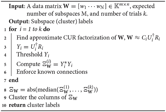
Proto-algorithm:. CUR Subspace Clustering

It should be evident that the reason for the term proto-algorithm is that several of the steps admit some ambiguity in their implementation. For instance, in line 2, how should one choose a CUR approximation to W? Many different ways of choosing columns and rows have been explored, e.g., by Drineas et al. [5], who choose rows and columns randomly according to a probability distribution favoring large columns or rows, respectively. On the other hand, Demanet and Chiu [38] show that uniformly selecting columns and rows can also perform quite well. In our subsequent experiments, we choose to select rows and columns uniformly at random.

There is yet more ambiguity in this step though, in that one has the flexibility to choose different numbers of columns and rows (as long as each number is at least the rank of W). Our choice of the number of rows and columns will be discussed in the next subsections.

Thirdly, the thresholding step in line 4 of the proto-algorithm deserves some attention. In experimentation, we tried a number of thresholds, many of which were based on the singular values of the data matrix W. However, the threshold that worked the best for motion data was a volumetric one based on the form of Y_i guaranteed by Theorem 3. Indeed, if there are M subspaces each of the same dimension, then Y_i should have precisely a proportion of $1-\frac{1}{M}$ of its total entries being 0. Thus our thresholding function orders the entries in descending order and keeps the top $(1-\frac{1}{M})\times$ (total # of entries), and sets the rest to 0.

Line 7 is simply a way to use any known information about the data to assist in the final clustering. Typically, no prior information is assumed other than the fact that we obviously know that w_i is in the same subspace as itself. Consequently here, we force the diagonal entries of Ξ_i to be 1 to emphasize that this connection is guaranteed.

The reason for the appearance of an averaging step in line 8 is that, while a similarity matrix formed from a single CUR approximation of a data matrix may contain many errors, this behavior should average out to give the correct clusters. The entrywise median of the family ${\left\{{\Xi }_{\text{W}}^{(i)}\right\}}_{i=1}^k$ is used rather than the mean to ensure more robustness to outliers. Note that a similar method of averaging CUR approximations was evaluated for denoising matrices in Sekmen et al. [65]; additional methods of matrix factorizations in matrix (or image) denoising may be found in Muhammad et al. [66], for example.

Note also that we do not take powers of the matrix $Y_i^{*}{Y}_i$ as suggested by Theorem 2. The reason for this is that when noise is added to the similarity matrix, taking the matrix product multiplicatively enhances the noise and greatly degrades the performance of the clustering algorithm. There is good evidence that taking elementwise products of a noisy similarity matrix can improve performance [26, 33]. This is really a different methodology than taking matrix powers, so we leave this discussion until later.

Finally, the clustering step in line 10 is there because at that point, we have a non-ideal similarity matrix Ξ_W, meaning that it will not exactly give the clusters because there are few entries which are actually 0. However, each column should ideally have large (i, j) entry whenever w_i and w_j are in the same subspace, and small (in absolute value) entries whenever w_i and w_j are not. This situation mimics what is done in Spectral Clustering, in that the matrix obtained from the first part of the Spectral Clustering algorithm does not have rows which lie exactly on the coordinate axes given by the eigenvectors of the graph Laplacian; however hopefully they are small perturbations of such vectors and a basic clustering algorithm like k–means can give the correct clusters. We discuss the performance of several different basic clustering algorithms used in this step in the sequel.

In the remainder of this section, the proto-algorithm above is investigated by first considering its performance on synthetic data, whereupon the initial findings are subsequently verified using the motion segmentation dataset known as Hopkins155 [67].

7.2. Simulations Using Synthetic Data

A set of simulations are designed using synthetic data. In order for the results to be comparable to that of the motion segmentation case presented in the following section, the data is constructed in a similar fashion. Particularly, in the synthetic experiments, data comes from the union of independent 4 dimensional subspaces of ℝ³⁰⁰. This corresponds to a feature being tracked for 5 s in a 30 fps video stream. Two cases similar to the ones in Hopkins155 dataset are investigated for increasing levels of noise. In the first case, two subspaces of dimension 4 are randomly generated, while in the second case three subspaces are generated. In both cases, the data is randomly drawn from the unit ball of the subspaces. In both cases, the level of noise on W is gradually increased from the initial noiseless state to the maximum noise level. The entries of the noise are i.i.d. ${N}(0,{\sigma }^2)$ random variables (i.e., with zero-mean and variance σ²), where the variance increases as σ = [0.000, 0.001, 0.010, 0.030, 0.050, 0.075, 0.10].

In each case, for each noise level, 100 data matrices are randomly generated containing 50 data vectors in each subspace. Once each data matrix W is formed, a similarity matrix Ξ_W is generated using the proto-algorithm for CUR subspace clustering. The parameters used are as follows: in the CUR approximation step (line 2), we choose all columns and the expected rank number of rows. Therefore, the matrix Y of Theorem 2 is of the form R^†R. The expected rank number of rows (i.e., the number of subspaces times 4) are chosen uniformly at random from W, and it is ensured that R has the expected rank before proceeding; the thresholding step (line 4) utilizes the volumetric threshold described in the previous subsection, so in Case 1 we eliminate half the entries of Y, while in Case 2 we eliminate 2/3 of the entries; we set k = 25, i.e. we compute 25 separate similarity matrices for each of the 100 data matrices and subsequently take the entrywise median of the 25 similarity matrices (line 8)—extensive testing shows no real improvement for larger values of k, so this value was settled on empirically; finally, we utilized three different clustering algorithms in line 10: k–means, Spectral Clustering [24], and Principal Coordinate Clustering (PCC) [68]. To spare unnecessary clutter, we only display the results of the best clustering algorithm in Figure 2, which turns out to be PCC, and simply state here that using Matlab's k–means algorithm gives very poor performance even at low noise levels, while Spectral Clustering gives good performance for low noise levels but degrades rapidly after about σ = 0.05. More specifically, k–means has a range of errors from 0 to 50% even for the σ = 0 in Case 2, while having an average of 36 and 48% clustering error in Case 1 and 2, respectively for the maximal noise level σ = 0.1. Meanwhile, Spectral Clustering exhibited on average perfect classification up to noise level σ = 0.03 in both cases, but jumped rapidly to an average of 12 and 40% error in Case 1 and 2, respectively for the case σ = 0.1. Figure 2 below shows the error plots for both cases when utilizing PCC. For a full description of PCC the reader is invited to consult [68], but essentially it eliminates the use of the graph Laplacian as in Spectral Clustering, and instead uses the principal coordinates of the first few left singular vectors in the singular value decomposition of Ξ_W. Namely, if Ξ_W has skinny SVD of order M (the number of subspaces) of $U_M{\Sigma }_M{V}_M^{*}$, then PCC clusters the rows of ${\Sigma }_M{V}_M^{*}$ using k–means.

Results for Case 1 and Case 2 using PCC are given in Figure 1. For illustration, Figure 2 shows the performance of a single CUR decomposition to form Ξ_W. As expected, the randomness involved in finding a CUR decomposition plays a highly nontrivial role in the clustering algorithm. It is remarkable to note, however, the enormity of the improvement the averaging procedure gives for higher noise levels, as can be seen by comparing the two figures.

FIGURE 1

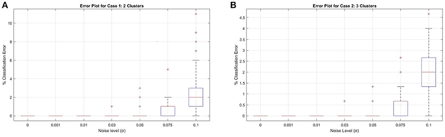
Figure 1. Synthetic Cases 1 and 2 for Ξ_W calculated using the median of 25 CUR decompositions. (A) Case 1, (B) Case 2.

FIGURE 2

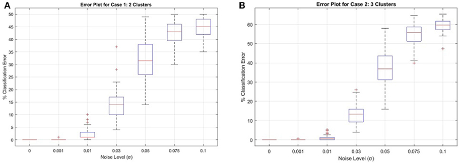
Figure 2. Synthetic Cases 1 and 2 for Ξ_W calculated using a single CUR decomposition. (A) Case 1, (B) Case 2.

7.3. Motion Segmentation Dataset: Hopkins155

The Hopkins155 motion dataset contains 155 videos which can be broken down into several categories: checkerboard sequences where moving objects are overlaid with a checkerboard pattern to obtain many feature points on each moving object, traffic sequences, and articulated motion (such as people walking) where the moving body contains joints of some kind making the 4-dimensional subspace assumption on the trajectories incorrect. Associated with each video is a data matrix giving the trajectories of all features on the moving objects (these features are fixed in advance for easy comparison). Consequently, the data matrix is unique for each video, and the ground truth for clustering is known a priori, thus allowing calculation of the clustering error, which is simply the percentage of incorrectly clustered feature points. An example of a still frame from one of the videos in Hopkins155 is shown in Figure 3. Here we are focused only on the clustering problem for motion data; however, there are many works on classifying motions in video sequences which are of a different flavor (e.g., [69–71]).

FIGURE 3

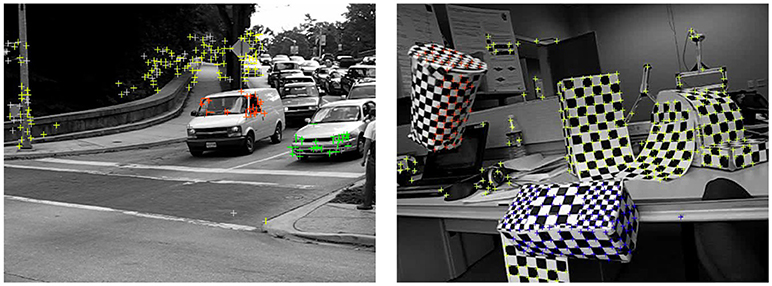
Figure 3. Example stills from a car sequence (left) and checkerboard sequence (right) from the Hopkins155 motion dataset.

As mentioned, clustering performance using CUR decompositions is tested using the Hopkins155 dataset. In this set of experiments, we use essentially the same parameters as discussed in the previous subsection when testing synthetic data. That is, we use CUR approximations of the form WR^†R where exactly the expected rank number of rows are chosen uniformly at random, the volumetric threshold is used, and we take the median of 50 similarity matrices for each of the 155 data matrices (we use k = 50 here instead of 25 to achieve a more robust performance on the real dataset). Again, PCC is favored over k–means and Spectral Clustering due to a dramatic increase in performance.

It turns out that for real motion data, CUR yields better overall results than SIM, the other pure similarity matrix method. This is reasonable given the flexibility of the CUR decomposition. Finding several similarity matrices and averaging them has the effect of averaging out some of the inherent noise in the data. The classification errors for our method as well as many benchmarks appear in Tables 1–3. Due to the variability of any single trial over the Hopkins155 dataset, the CUR data presented in the tables is the average of 20 runs of the algorithm over the entire dataset. The purpose of this work is not to fine tune CUR's performance on the Hopkins155 dataset; nonetheless, the results using this simple method are already better than many of those in the literature.

TABLE 1

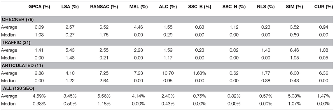
Table 1. % classification errors for sequences with two motions.

TABLE 2

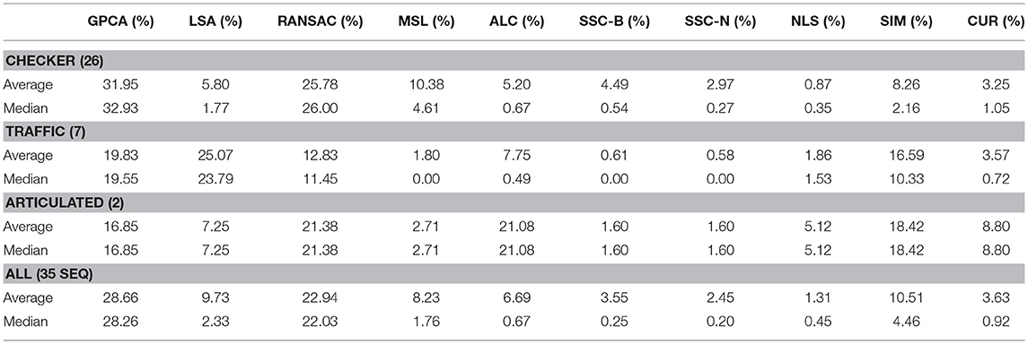
Table 2. % classification errors for sequences with three motions.

TABLE 3

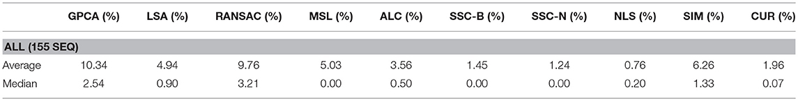
Table 3. % classification errors for all sequences.

To better compare performance, we timed the CUR-based method described above in comparison with some of the benchmark timings given in Tron and Vidal [67]. For direct comparison, we ran all of the algorithms on the same machine, which was a mid-2012 Macbook Pro with 2.6 GHz Intel Core i7 processor and 8GB of RAM. The results are listed in Table 4. We report the times for various values of k as in Step 1 of the Proto-algorithm, indicating how many CUR approximations are averaged to compute the similarity matrix.

TABLE 4

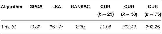
Table 4. Run times (in s) over the entire Hopkins155 dataset for various algorithms.

7.4. Discussion

It should be noted that after thorough experimentation on noisy data, using a CUR decomposition which takes all columns and exactly the expected rank number of rows exhibits the best performance. That is, a decomposition of the form W = WR^†R performs better on average than one of the form W = CU^†R. The fact that choosing more columns performs better when the matrix W is noisy makes sense in that any representation of the form W = CX is a representation of W in terms of the frame vectors of C. Consequently, choosing more columns in the matrix C means that we are adding redundancy to the frame, and it is well-known to be one of the advantages of frame representations that redundancy provides greater robustness to noise. Additionally, we noticed experimentally that choosing exactly r rows in the decomposition WR^†R exhibits the best performance. It is not clear as of yet why this is the case.

As seen in the tables above, the proposed CUR based clustering algorithm works dramatically better than SIM, but does not beat the best state-of-the-art obtained by the first and fourth author in Aldroubi and Sekmen [72]. More investigation is needed to determine if there is a way to utilize the CUR decomposition in a better fashion to account for the noise. Of particular interest may be to utilized convex relaxation method recently proposed in Li et al. [54].

One interesting note from the results in the tables above is that, while some techniques for motion clustering work better on the checkered sequences rather than traffic sequences (e.g., NLS, SSC, and SIM), CUR seems to be blind to this difference in the type of data. It would be interesting to explore this phenomenon further to determine if the proposed method performs uniformly for different types of motion data. We leave this task to future research.

As a final remark, we note that the performance of CUR decreases as k, the number of CUR decompositions averaged to obtain the similarity matrix, increases. The error begins to level out beyond about k = 50, whereas the time steadily increases as k does (see Table 4). One can easily implement an adaptive way of choosing k for each data matrix rather than holding it fixed. To test this, we implemented a simple threshold by taking, for each i in the Proto-algorithm, a temporary similarity matrix ${\tilde{\Xi }}_{\text{W}}^{(i)}:=\text{abs(median}({\Xi }_{\text{W}}^{(1)},\dots {\Xi }_{\text{W}}^{(i)}))$. That is, ${\tilde{\Xi }}_{\text{W}}^{(i)}$ is the median of all of the CUR similarity matrices produced thus far in the for loop. We then computed $\left|\right|{\tilde{\Xi }}_{\text{W}}^{(i)}-{\tilde{\Xi }}_{\text{W}}^{(i-1)}|{|}_2$, and compared it to a threshold (in this case 0.01). If the norm was less than the threshold, then we stopped the for loop, and if not we kept going, setting an absolute cap of 100 on the number of CUR decompositions used. We found that on average, 57 CUR decompositions were used, with a minimum of 37, a maximum of 100 (the threshold value), and a standard deviation of 13. Thus it appears that a roughly optimal region for fast time performance and good clustering accuracy is around k = 50 to k = 60 CUR decompositions.

7.5. Robust CUR Similarity Matrix for Subspace Clustering

We now turn to a modification of the Proto-algorithm discussed above. One of the primary reasons for using the CUR decomposition as opposed to the shape interaction matrix ($V_r{V}_r^{*}$) is that the latter is not robust to noise. However, Ji et al. [33] proposed a robustified version of SIM, called RSIM. The key feature of their algorithm is that they do not enforce the clustering rank beforehand, but they find a range of possible ranks, and make a similarity matrix for each rank in this range, and perform Spectral Clustering on a modification of the SIM. Then, they keep the clustering labels from the similarity matrix for the rank r which minimizes the associated minCut quantity on the graph determined by the similarity matrix.

Recall given a weighted, undirected graph G = (V, E), and a partition of its vertices, {A₁, …, A_k}, the Ncut value of the partition is

${\mathrm{\text{Ncut}}}_k(A_1,\dots ,A_k):=\frac{1}{2}{\displaystyle \sum _{i=1}^k}\frac{W(A_i,A_i^C)}{\mathrm{\text{vol}}(A_i)},$

where $W(A,A^C):=\sum _{i\in A,j\in A^C}{w}_{i,j}$, where w_{i, j} is the weight of the edge (v_i, v_j) (defined to be 0 if no such edge exists). The RSIM method varies the rank r of the SIM (i.e. the rank of the SVD taken), and minimizes the corresponding Ncut quantity over r.

The additional feature of the RSIM algorithm is that rather than simply taking $V_r{V}_r^{*}$ for the similarity matrix, they first normalize the rows of V_r and then take elementwise power of the resulting matrix. This follows the intuition of Lauer and Schnorr [26] and should be seen as a type of thresholding as in Step 4 of the Proto-algorithm. For the full RSIM algorithm, consult [33], but we present the CUR analog that maintains most of the steps therein.

The main difference between Algorithm 1 and that of Ji et al. [33] is that in the latter, Steps 2–8 in Algorithm 1 are replaced with computing the thin SVD of order r, and normalizing the rows of V_r, and then setting ${\Xi }_{\text{W}}=V_r{V}_r^{*}$. In Ji et al. [33], the Normalized Cuts clustering algorithm is preferred, which is also called Spectral Clustering with the symmetric normalized graph Laplacian [24]. In our testing of RCUR, it appears that the normalization and elementwise powering steps interfere with the principal coordinate system in PC clustering; we therefore used Spectral Clustering as in the RSIM case. Results are presented in Tables 5–7. Note that the values for RSIM may differ from those reported in Ji et al. [33]; there the authors only presented errors for all 2–motion sequences, all 3–motion sequences, and overall rather than considering each subclass (e.g., checkered or traffic). We used the code from [33] for the values specified by their algorithm and report its performance in the tables below (in general, the values reported here are better than those in [33]).

Algorithm 1

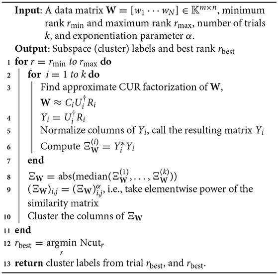
Algorithm 1: Robust CUR Similarity Matrix (RCUR)

TABLE 5

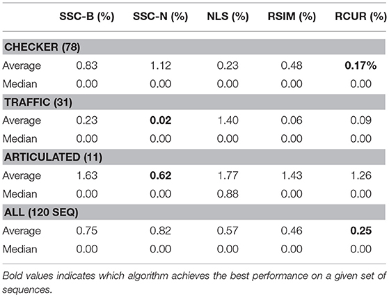
Table 5. % classification errors for sequences with two motions.

TABLE 6

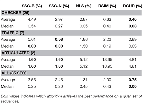
Table 6. % classification errors for sequences with three motions.

TABLE 7

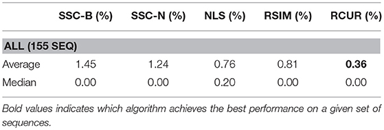
Table 7. % classification errors for all sequences.

The results displayed in the table are obtained by choosing k = 50 to be fixed (based on the analysis in the previous section), and taking CUR factorizations of the form $\text{W}\approx C_i{R}_i^{†}{R}_i$, where we choose r rows to form R_i, where r is given in Step 1 of the algorithm. This is, by Corollary 5, the theoretical equivalent of taking $V_r{V}_r^{*}$ as in RSIM. Due to the randomness of finding CUR factorizations in Algorithm 1, the algorithm was run 20 times and the average performance was reported in Tables 5–7. We note also that the standard deviation of the performance across the 20 trials was less than 0.5% for all categories with the exception of the Articulated 3 motion category, in which case the standard deviation was large (5.48%).

As can be seen, the algorithm proposed here does not yield the best performance on all facets of the Hopkins155 dataset; however, it does achieve the best overall classification result to date with only 0.36% average classification error. As an additional note, running Algorithm 1 with only k = 10 CUR factorizations used for each data matrix still yields relatively good results (total 2–motion error of 0.41%, total 3–motion error of 1.21%, and total error on all of Hopkins155 of 0.59%) while allowing for less computation time. Preliminary tests suggest also that taking fewer rows in the CUR factorization step in Algorithm 1 works much better than in the version of the Proto-algorithm used in the previous sections (for instance, taking half of the available columns and r rows still yields <0.5% overall error). However, the purpose of the current work is not to optimize all facets of Algorithm 1, as much more experimentation needs to be done to determine the correct parameters for the algorithm, and it needs to be tested on a broad variety of datasets which approximately satisfy the union of subspaces assumption herein considered. This task we leave to future work.

8. Concluding Remarks

The motivation of this work was truly the realization that the exact CUR decomposition of Theorem 1 can be used for the subspace clustering problem. We demonstrated that, on top of its utility in randomized linear algebra, CUR enjoys a prominent place atop the landscape of solutions to the subspace clustering problem. CUR provides a theoretical umbrella under which sits the known shape interaction matrix, but it also provides a bridge to other solution methods inspired by compressed sensing, i.e., those involving the solution of an ℓ₁ minimization problem. Moreover, we believe that the utility of CUR for clustering and other applications will only increase in the future. Below, we provide some reasons for the practical utility of CUR decompositions, particularly related to data analysis and clustering, as well as some future directions.

Benefits of CUR:

• From a theoretical standpoint, the CUR decomposition of a matrix is utilizing a frame structure rather than a basis structure to factorize the matrix, and therefore enjoys a level of flexibility beyond something like the SVD. This fact should provide utility for applications.

• Additionally, a CUR decomposition remains faithful to the structure of the data. For example, if the given data is sparse, then both C and R will be sparse, even if U^† is not in general. In contrast, taking the SVD of a sparse matrix yields full matrices U and V, in general.

• Often in obtaining real data, many entries may be missing or extremely corrupted. In motion tracking, for example, it could be that some of the features are obscured from view for several frames. Consequently, some form of matrix completion may be necessary. On the other hand, a look at the CUR decomposition reveals that whole rows of a data matrix can be missing as long as we can still choose enough rows such that the resulting matrix R has the same rank as W.

Future Directions

• Algorithm 1 and other iterations of the Proto-algorithm presented here need to be further tested to determine the best way to utilize the CUR decomposition to cluster subspace data. Currently, Algorithm 1 is somewhat heuristic, so a more fully understood theory concerning its performance is needed. We note that some justification for the ideas of RSIM are given in Ji et al. [33]; however, the ideas there do not fully explain the outstanding performance of the algorithm. As commented above, one of the benefits of the Proto-algorithm discussed here is its flexibility, which provides a distinct advantage over SVD based methods.

• Another direction is to combine the CUR technique with sparse methods to construct algorithms that are strongly robust to noise and that allow clustering when the data points are not drawn from a union of independent subspaces.

Author Contributions

All authors listed have made a substantial, direct and intellectual contribution to the work, and approved it for publication.

Conflict of Interest Statement

The authors declare that the research was conducted in the absence of any commercial or financial relationships that could be construed as a potential conflict of interest.

Acknowledgments

The research of AS and AK is supported by DoD Grant W911NF-15-1-0495. The research of AA is supported by NSF Grant NSF/DMS 1322099. The research of AK is also supported by TUBITAK-2219-1059B191600150. Much of the work for this article was done while KH was an assistant professor at Vanderbilt University. In the final stage of the project, the research of KH was partially supported through the NSF TRIPODS project under grant CCF-1423411.

The authors also thank the referees for constructive comments which helped improve the quality of the manuscript.

References

1. Mahoney MW, Drineas P. CUR matrix decompositions for improved data analysis. Proc Natl Acad Sci USA. (2009) 106:697–702. doi: 10.1073/pnas.0803205106

PubMed Abstract | CrossRef Full Text | Google Scholar

2. Boutsidis C, Woodruff DP. Optimal CUR matrix decompositions. SIAM J Comput. (2017) 46:543–89. doi: 10.1137/140977898

CrossRef Full Text | Google Scholar

3. Drineas P, Kannan R, Mahoney MW. Fast Monte Carlo algorithms for matrices I: approximating matrix multiplication. SIAM J Comput. (2006) 36:132–57. doi: 10.1137/S0097539704442684

CrossRef Full Text | Google Scholar

4. Drineas P, Kannan R, Mahoney MW. Fast Monte Carlo algorithms for matrices II: computing a low-rank approximation to a matrix. SIAM J Comput. (2006) 36:158–83. doi: 10.1137/S0097539704442696

CrossRef Full Text | Google Scholar

5. Drineas P, Kannan R, Mahoney MW. Fast Monte Carlo algorithms for matrices III: computing a compressed approximate matrix decomposition. SIAM J Comput. (2006) 36:184–206. doi: 10.1137/S0097539704442702

CrossRef Full Text | Google Scholar

6. Georghiades AS, Belhumeur PN, Kriegman DJ. From few to many: illumination cone models for face recognition under variable lighting and pose. IEEE Trans Pattern Anal Mach Intell. (2001) 23:643–60. doi: 10.1109/34.927464

CrossRef Full Text | Google Scholar

7. Basri R, Jacobs DW. Lambertian reflectance and linear subspaces. IEEE Trans Pattern Anal Mach Intell. (2003) 25:218–33. doi: 10.1109/TPAMI.2003.1177153

CrossRef Full Text | Google Scholar

8. Kanatani K, Sugaya Y. Multi-stage optimization for multi-body motion segmentation. In: IEICE Transactions on Information and Systems (2003). p. 335–49.

Google Scholar

9. Aldroubi A, Zaringhalam K. Nonlinear least squares in ℝⁿ. Acta Appl Math. (2009) 107:325–37. doi: 10.1007/s10440-008-9398-9

CrossRef Full Text | Google Scholar

10. Aldroubi A, Cabrelli C, Molter U. Optimal non-linear models for sparsity and sampling. J Four Anal Appl. (2009) 14:793–812. doi: 10.1007/s00041-008-9040-2

CrossRef Full Text | Google Scholar

11. Tseng P. Nearest q-flat to m points. J Optim Theory Appl. (2000) 105:249–52. doi: 10.1023/A:1004678431677

CrossRef Full Text | Google Scholar

12. Fischler M, Bolles R. Random sample consensus: a paradigm for model fitting with applications to image analysis and automated cartography. Commun ACM (1981) 24:381–95. doi: 10.1145/358669.358692

CrossRef Full Text | Google Scholar

13. Silva N, Costeira J. Subspace segmentation with outliers: a Grassmannian approach to the maximum consensus subspace. In: IEEE Computer Society Conference on Computer Vision and Pattern Recognition. Anchorage, AK (2008).

Google Scholar

14. Zhang T, Szlam A, Wang Y, Lerman G. Randomized hybrid linear modeling by local best-fit flats. In: IEEE Conference on Computer Vision and Pattern Recognition. San Fransisco, CA (2010). p. 1927–34.

Google Scholar

15. Zhang YW, Szlam A, Lerman G. Hybrid linear modeling via local best-fit flats. Int J Comput Vis. (2012) 100:217–40. doi: 10.1007/s11263-012-0535-6

CrossRef Full Text | Google Scholar

16. Vidal R, Ma Y, Sastry S. Generalized Principal Component Analysis (GPCA). IEEE Trans Pattern Anal Mach Intell. (2005) 27:1945–59. doi: 10.1109/TPAMI.2005.244

PubMed Abstract | CrossRef Full Text | Google Scholar

17. Ma Y, Yang AY, Derksen H, Fossum R. Estimation of subspace arrangements with applications in modeling and segmenting mixed data. SIAM Rev. (2008) 50:1–46. doi: 10.1137/060655523

CrossRef Full Text | Google Scholar

18. Tsakiris MC, Vidal R. Filtrated spectral algebraic subspace clustering. SIAM J Imaging Sci. (2017) 10:372–415. doi: 10.1137/16M1083451

CrossRef Full Text | Google Scholar

19. Eldar YC, Mishali M. Robust recovery of signals from a structured union of subspaces. IEEE Trans Inform Theory (2009) 55:5302–16. doi: 10.1109/TIT.2009.2030471

CrossRef Full Text | Google Scholar

20. Elhamifar E, Vidal R. Sparse subspace clustering. In: IEEE Conference on Computer Vision and Pattern Recognition. Miami, FL (2009). p. 2790–97.

PubMed Abstract | Google Scholar

21. Elhamifar E, Vidal R. Clustering disjoint subspaces via sparse representation. In: IEEE International Conference on Acoustics, Speech, and Signal Processing (2010).

Google Scholar

22. Liu G, Lin Z, Yu Y. Robust subspace segmentation by low-rank representation. In: International Conference on Machine Learning. Haifa (2010). p. 663–70.

Google Scholar

23. Liu G, Lin Z, Yan S, Sun J, Yu Y, Ma Y. Robust recovery of subspace structures by low-rank representation. IEEE Trans Pattern Anal Mach Intell. (2013) 35:171–84. doi: 10.1109/TPAMI.2012.88

PubMed Abstract | CrossRef Full Text | Google Scholar

24. Luxburg UV. A tutorial on spectral clustering. Stat Comput. (2007) 17:395–416. doi: 10.1007/s11222-007-9033-z

CrossRef Full Text | Google Scholar

25. Chen G, Lerman G. Spectral Curvature Clustering (SCC). Int J Comput Vis. (2009) 81:317–30. doi: 10.1007/s11263-008-0178-9

CrossRef Full Text | Google Scholar

26. Lauer F, Schnorr C. Spectral clustering of linear subspaces for motion segmentation. In: IEEE International Conference on Computer Vision. Kyoto (2009).

Google Scholar

27. Yan J, Pollefeys M. A general framework for motion segmentation: independent, articulated, rigid, non-rigid, degenerate and nondegenerate. In: 9th European Conference on Computer Vision. Graz (2006). p. 94–106.

Google Scholar

28. Goh A, Vidal R. Segmenting motions of different types by unsupervised manifold clustering. In: IEEE Conference on Computer Vision and Pattern Recognition, 2007. CVPR '07. Minneapolis, MN (2007). p. 1–6.

Google Scholar

29. Chen G, Lerman G. Foundations of a multi-way spectral clustering framework for hybrid linear modeling. Found Comput Math. (2009) 9:517–58. doi: 10.1007/s10208-009-904

CrossRef Full Text | Google Scholar

30. Vidal R. A tutorial on subspace clustering. IEEE Signal Process Mag. (2010) 28:52–68. doi: 10.1109/MSP.2010.939739

CrossRef Full Text | Google Scholar

31. Aldroubi A, Sekmen A, Koku AB, Cakmak AF. Similarity Matrix Framework for Data from Union of Subspaces. Appl Comput Harmon Anal. (2018) 45:425–35. doi: 10.1016/j.acha.2017.08.006

CrossRef Full Text | Google Scholar

32. Costeira J, Kanade T. A multibody factorization method for independently moving objects. Int J Comput Vis. (1998) 29:159–79. doi: 10.1023/A:1008000628999

CrossRef Full Text | Google Scholar

33. Ji P, Salzmann M, Li H. Shape interaction matrix revisited and robustified: efficient subspace clustering with corrupted and incomplete data. In: Proceedings of the IEEE International Conference on Computer Vision. Santiago (2015). p. 4687–95.

Google Scholar

34. Golub GH, Van Loan CF. Matrix Computations, Vol. 3. JHU Press (2012).

Google Scholar

35. Alexeev B, Cahill J, Mixon DG. Full spark frames. J Fourier Anal Appl. (2012) 18:1167–94. doi: 10.1007/s00041-012-9235-4

CrossRef Full Text | Google Scholar

36. Donoho DL, Elad M. Optimally sparse representation in general (nonorthogonal) dictionaries via 1 minimization. Proc Natl Acad Sci USA. (2003) 100:2197–202. doi: 10.1073/pnas.0437847100

CrossRef Full Text | Google Scholar

37. Goreinov SA, Zamarashkin NL, Tyrtyshnikov EE. Pseudo-skeleton approximations by matrices of maximal volume. Math Notes (1997) 62:515–9. doi: 10.1007/BF02358985

CrossRef Full Text | Google Scholar

38. Chiu J, Demanet L. Sublinear randomized algorithms for skeleton decompositions. SIAM J Matrix Anal Appl. (2013) 34:1361–83. doi: 10.1137/110852310

CrossRef Full Text | Google Scholar

39. Goreinov SA, Tyrtyshnikov EE, Zamarashkin NL. A theory of pseudoskeleton approximations. Linear Algebra Appl. (1997) 261:1–21. doi: 10.1016/S0024-3795(96)00301-1

CrossRef Full Text | Google Scholar

40. Caiafa CF, Cichocki A. Generalizing the column–row matrix decomposition to multi-way arrays. Linear Algebra Appl. (2010) 433:557–73. doi: 10.1016/j.laa.2010.03.020

CrossRef Full Text | Google Scholar

41. Gantmacher FR. Theory of Matrices. 2V. Chelsea Publishing Company (1960).

Google Scholar

42. Penrose R. On best approximate solutions of linear matrix equations. Math Proc Cambridge Philos Soc. (1956) 52:17–9. doi: 10.1017/S0305004100030929

CrossRef Full Text | Google Scholar

43. Stewart G. Four algorithms for the the efficient computation of truncated pivoted QR approximations to a sparse matrix. Numer Math. (1999) 83:313–23. doi: 10.1007/s002110050451

CrossRef Full Text | Google Scholar

44. Berry MW, Pulatova SA, Stewart G. Algorithm 844: computing sparse reduced-rank approximations to sparse matrices. ACM Trans Math Soft. (2005) 31:252–69. doi: 10.1145/1067967.1067972

CrossRef Full Text | Google Scholar

45. Wang S, Zhang Z. Improving CUR matrix decomposition and the Nyström approximation via adaptive sampling. J Mach Learn Res. (2013) 14:2729–69. Available online at: http://www.jmlr.org/papers/volume14/wang13c/wang13c.pdf

Google Scholar

46. Drineas P, Mahoney MW, Muthukrishnan S. Relative-error CUR matrix decompositions. SIAM J Matrix Anal Appl. (2008) 30:844–81. doi: 10.1137/07070471X

CrossRef Full Text | Google Scholar

47. Voronin S, Martinsson PG. Efficient algorithms for cur and interpolative matrix decompositions. Adv Comput Math. (2017) 43:495–516. doi: 10.1007/s10444-016-9494-8

CrossRef Full Text | Google Scholar

48. Wang S, Zhang Z, Zhang T. Towards more efficient SPSD matrix approximation and CUR matrix decomposition. J Mach Learn Res. (2016) 17:1–49. Available online at: http://www.jmlr.org/papers/volume17/15-190/15-190.pdf

Google Scholar

49. Oswal U, Jain S, Xu KS, Eriksson B. Block CUR: decomposing large distributed matrices. arXiv [Preprint]. arXiv:170306065. (2017).

Google Scholar

50. Li X, Pang Y. Deterministic column-based matrix decomposition. IEEE Trans Knowl Data Eng. (2010) 22:145–9. doi: 10.1109/TKDE.2009.64

CrossRef Full Text | Google Scholar

51. Yip CW, Mahoney MW, Szalay AS, Csabai I, Budavári T, Wyse RF, et al. Objective identification of informative wavelength regions in galaxy spectra. Astron J. (2014) 147:110. doi: 10.1088/0004-6256/147/5/110

CrossRef Full Text | Google Scholar

52. Yang J, Rubel O, Mahoney MW, Bowen BP. Identifying important ions and positions in mass spectrometry imaging data using CUR matrix decompositions. Anal Chem. (2015) 87:4658–66. doi: 10.1021/ac5040264

PubMed Abstract | CrossRef Full Text | Google Scholar

53. Xu M, Jin R, Zhou ZH. CUR algorithm for partially observed matrices. In: International Conference on Machine Learning. Lille (2015). p. 1412–21.

Google Scholar

54. Li C, Wang X, Dong W, Yan J, Liu Q, Zha H. Joint active learning with feature selection via CUR matrix decomposition. In: IEEE Transactions on Pattern Analysis and Machine Intelligence. (2018). doi: 10.1109/TPAMI.2018.2840980

PubMed Abstract | CrossRef Full Text | Google Scholar

55. Halko N, Martinsson PG, Tropp JA. Finding structure with randomness: probabilistic algorithms for constructing approximate matrix decompositions. SIAM Rev. (2011) 53:217–88. doi: 10.1137/090771806

CrossRef Full Text | Google Scholar

56. Muhammad N, Bibi N. Digital image watermarking using partial pivoting lower and upper triangular decomposition into the wavelet domain. IET Image Process. (2015) 9:795–803. doi: 10.1049/iet-ipr.2014.0395

CrossRef Full Text | Google Scholar

57. Muhammad N, Bibi N, Qasim I, Jahangir A, Mahmood Z. Digital watermarking using Hall property image decomposition method. Pattern Anal Appl. (2018) 21:997–1012. doi: 10.1007/s10044-017-0613-z

CrossRef Full Text | Google Scholar

58. Otazo R, Candès E, Sodickson DK. Low-rank plus sparse matrix decomposition for accelerated dynamic MRI with separation of background and dynamic components. Magn Reson Med. (2015) 73:1125–36. doi: 10.1002/mrm.25240

PubMed Abstract | CrossRef Full Text | Google Scholar

59. Candes EJ, Plan Y. Matrix completion with noise. Proc IEEE. (2010) 98:925–36. doi: 10.1109/JPROC.2009.2035722

CrossRef Full Text | Google Scholar

60. Wei S, Lin Z. Analysis and improvement of low rank representation for subspace segmentation. arXiv [Preprint]. arXiv:1107.1561 [cs.CV] (2011).

Google Scholar

61. Meka R, Jain P, Caramanis C, Dhillon IS. Rank minimization via online learning. In: Proceedings of the 25th International Conference on Machine Learning. Helsinki (2008). p. 656–63.

Google Scholar

62. Recht B, Xu W, Hassibi B. Necessary and sufficient conditions for success of the nuclear norm heuristic for rank minimization. In: 47th IEEE Conference on Decision and Control, 2008. CDC 2008. Cancun (2008). p. 3065–70.

Google Scholar

63. Recht B, Xu W, Hassibi B. Null space conditions and thresholds for rank minimization. Math Programm. (2011) 127:175–202. doi: 10.1007/s10107-010-0422-2

CrossRef Full Text | Google Scholar

64. Kanatani K, Matsunaga C. Estimating the number of independent motions for multibody motion segmentation. In: 5th Asian Conference on Computer Vision. Melbourne, VIC (2002). p. 7–9.

Google Scholar

65. Sekmen A, Aldroubi A, Koku AB, Hamm K. Matrix reconstruction: skeleton decomposition versus singular value decomposition. In: 2017 International Symposiu on Performance Evaluation of Computer and Telecommunication Systems (SPECTS). Seattle, WA (2017). p. 1–8.

Google Scholar

66. Muhammad N, Bibi N, Jahangir A, Mahmood Z. Image denoising with norm weighted fusion estimators. Pattern Anal Appl. (2018) 21:1013–22. doi: 10.1007/s10044-017-0617-8

CrossRef Full Text | Google Scholar

67. Tron R, Vidal R. A benchmark for the comparison of 3-D motion segmentation algorithms. In: IEEE Conference on Computer Vision and Pattern Recognition. Minneapolis, MN (2007). p. 1–8.

Google Scholar

68. Sekmen A, Aldroubi A, Koku AB, Hamm K. Principal coordinate clustering. In: 2017 IEEE International Conference on Big Data (Big Data). Boston, MA (2017). p. 2095–101.

Google Scholar

69. Cho K, Chen X. Classifying and visualizing motion capture sequences using deep neural networks. In: 2014 International Conference on Computer Vision Theory and Applications (VISAPP), Vol. 2. Lisbon (2014). p. 122–30.

Google Scholar

70. Khan MA, Akram T, Sharif M, Javed MY, Muhammad N, Yasmin M. An implementation of optimized framework for action classification using multilayers neural network on selected fused features. Pattern Anal Appl. (2018) 1–21. doi: 10.1007/s10044-018-0688-1

CrossRef Full Text

71. Arn R, Narayana P, Draper B, Emerson T, Kirby M, Peterson C. Motion Segmentation via Generalized Curvatures. In: IEEE Transactions on Pattern Analysis and Machine Intelligence (2018).

PubMed Abstract | Google Scholar

72. Aldroubi A, Sekmen A. Nearness to local subspace algorithm for subspace and motion segmentation. IEEE Signal Process Lett. (2012) 19:704–7. doi: 10.1109/LSP.2012.2214211

CrossRef Full Text | Google Scholar