Measuring Dynamical Uncertainty With Revealed Dynamics Markov Models

1. Introduction

Time series uncertainty is a quantification of how complicated, complex, or difficult it is to predict or generate the sequence of values in the time series. Measures of time series uncertainty can be used to classify and identify changes in the characteristic behavior of time series. Applications that have utilized dynamical uncertainty-based categorization include identifying cardiac arrhythmias [1], epileptic patters in EEGs [2, 3], and shocks in financial dynamics [4] to name a few; and with the growth of machine learning techniques to classify behavior by quantified feature descriptions, there is a growing demand for accurate, robust, and scalable measures of time series dynamics.

Existing measures of time series uncertainty/complexity/predictability (used interchangeably in this context, henceforth just “uncertainty”) such as Approximate Entropy (ApEn) [5] and its refinement Sample Entropy (SampEn) [6] as well as Permutation [7] and Increment [8] entropies partially succeed by capturing specific features of time series dynamics, but they ignore other features that clearly contribute to a time series' uncertainty. This paper introduces a novel way to measure dynamical uncertainty in time series data by first converting its coarse-grained phase space into a descriptive Markov model called a “Revealed Dynamics Markov Model” (RDMM). Although predictive Markov models have been overshadowed by more sophisticated methods, they still hold many benefits for descriptive purposes: such as facilitating distance metrics and intuitively representing system dynamics [9]. Here we describe the mathematical foundation and robustness of the proposed approach to measuring uncertainty and demonstrate that it (1) is a genuine measure of time series uncertainty, (2) reflects distinct features of the dynamics compared to previous measures (3) results in improved classification of time series dynamics.

We first describe the construction of the specialized Markov model and the three proposed uncertainty measures on it: Shannon entropy, uniformity, and turbulence (effective edge density). We then explore the effects of binning parameters through a comparison against previous measures on simulated and empirical data. We find that the proposed measures are indeed distinct measures of uncertainty, and that many RDMM-based measures out-perform previous measures in accurately classifying time series by their uncertainty properties. We also individually evaluate the various RDMM-based measures and find that turbulence with a curvature parameter of 2 is the most consistent in accurately measuring dynamical uncertainty. We identify issues with binning and normalization that require further examination and point to applications in time series classification and event detection.

2. Methods

The proposed measurement technique operates on a description of the time series as a specific kind of Markov model. The construction of the requisite Markov model is straightforward; see Figure 1 for a simplified example. One coarse-grains the phase space and assigns a node for each non-empty bin; i.e., each observed system state. The frequency of each observed state transition is recorded on the edge between the corresponding nodes, and these frequencies are normalized to generate conditional probability distributions. That is, for each state we know the proportions of transitions over next states, and these proportions comprise the maximum likelihood estimates for the transition probabilities (although Laplacian, Bayesian, and other approaches exist). Any node without an exit transition is given a reflexive edge with weight 1 to ensure the result is a true Markov model of the revealed dynamics across the dataset's phase space (a “Revealed Dynamics Markov Model” or RDMM).

FIGURE 1

Figure 1. Simple demonstration of applying the RDMM method to a small sequence of data. Note that there are no observations in bin 3, so no node is created for it. The probabilities for each exit transition reflect the proportions of bin-to-bin changes except for bin 5′s terminating self-loop.

The analyses here use the simplest binning technique. For each dimension of time series X = {x₁, x₂, …, x_T} divide the observed range (maxx_i−minx_i) into B equal-width bins. This creates n nodes representing equivalence classes of values; but since some bins may be empty, $n\le {\prod }_{d=1}^D{B}_d$ for a phase space with dimension D (the bins per dimension/variable may be heterogeneous). Alternative binning methods collect different sets of points into each bin, and thus create different nodes and transitions, but the analysis of the resulting RDMM is unchanged.

As usual, node (state) s_i transitions to node s_j with probability p_ij. Because Markov models are directed, reflexive networks, when the set of nodes N is fully connected, the set of edges E has size n². No measure here is sensitive to a node's in-degree, so k_i will be used to refer solely to a node's out-degree, and k_i to the set of nodes that i can transition into:

$\begin{array}{cc}{k}_i={\cup }_{s_j\in N}{p}_{ij}>0.& (1)\end{array}$

Self-loops count in the out-degree of a node, thus k_i = |k_i|.

This RDMM variant of Markov modeling is essentially how one builds Markov chains from categorical data such as gene sequences [10], computer security profiles [11], and protein configurations [12], but here the nodes represent bins rather than predefined categories or events. Unlike hidden Markov models (HMMs) [13–16] where the nodes represent a combination of observable and unobservable (hidden) variables according to a user-specified model, the nodes of an RDMM are all derived from observable variables and no a priori model of their relationships is required. HMMs are used for tasks such as prediction, pattern recognition, and to infer the generative properties of the hidden nodes. The RDMMs proposed here capture and describe the observed time series, and can be used for pattern recognition and classification, but are not being proposed for predictive or inductive purposes. Other Markov chain approaches capture yet other features of the dynamics [17–19], highlighting how broadly useful the mathematical structure is.

Other network representations of time-series data exist as well: recurrence networks [20], networks of interacting dynamical units [21], networks of temporal correlations of data features (e.g., cycles [22]), and others (see [23] for a partial comparison). Depending on how the data are translated into a network, different network measures (such as degree, clustering coefficient, or betweenness centrality) are relevant and revealing; the Markov representation is a flexible framework for capturing time series data (especially simulation output) that is also useful for measuring other dynamical properties.

2.1. Measures of Dynamical Uncertainty on RDMMs

The Markov model representation enables techniques that combine structural measures of weighted directed graphs and probabilistic measures of stochastic processes. Although the mathematics necessary here are familiar, by combining well-understood ingredients in a novel way we produce a new analytical window on system dynamics. We propose the following desiderata for uncertainty measures on Markov models:

1. Uncertainty is maximized when all states are equally likely to transition into every state; this requires not just randomness, but a uniform distribution across all sequential pairs of data.

2. Uncertainty is minimized when every state has exactly one exit transition (including reflexive transitions); this implies that the process is deterministic, although not all deterministic processes will achieve this due to binning and/or hysteresis.

3. The measure reports (monotonically) higher values if and only if the uncertainty/complexity of the data is greater.

From an information-content interpretation these measures are similar to Kolmogorov (algorithmic) complexity in which the “program language” is a Markov model; what these measures tell us is how complicated that model has to be (in terms of the number and distributions of edges) in order to generate the time series data. RDMMs are intended to be merely descriptive (rather than predictive or generative), so what is important is that the RDMM appropriately captures the features bearing the uncertainty, and the measures track those uncertainty properties in the RDMM. We now present the mathematical details of the proposed measures, an evaluation of their satisfaction of the above desiderata, and a summary of comparison measures before moving on to the tests.

2.1.1. Entropy

The default measure of uncertainty is entropy, and more specifically Shannon entropy. Although Shannon entropy is commonly applied to Markov processes (including the original description in [24]), the Markov models in those applications are constructed distinctly from RDMMs; for example, they are required to be ergodic. RDMMs are often non-ergodic, but despite this difference the Shannon entropy measure is applicable and useful here after appropriate normalization and reinterpretation.

Entropy can be evaluated for individual nodes or for the whole system. For the local measure we calculate the entropy of the edge weights of the existing out-going transitions, but this doesn't adjust for the number of possible edges. For this application one must realize that missing links in an RDMM also provide information about the uncertainty of the system. As such, the appropriate measure of uncertainty must normalize over all n possible connections. The maximum entropy value occurs when a node's exit transitions are all equally weighted at p_ij = 1/k_i = 1/n. The equation for calculating normalized local entropy for each node is

$\begin{array}{cc}h(s_i)=\frac{1}{\ln \frac{1}{n}}{\displaystyle \sum _{s_j\in k_i}{p}_{ij}}\ln p_{ij}.& (2)\end{array}$

The entropy of the whole system H(S) can be equivalently calculated as either the mean of the node's individual entropy values or directly as the entropy of all the graph edges normalized by nln (1/n).

$\begin{array}{cc}\begin{array}{l}H(\text{S})=\frac{1}{nln\frac{1}{n}}{\displaystyle \sum _{i\in \text{E}}}{p}_{i}ln{p}_i.\end{array}& (3)\end{array}$

2.1.2. Uniformity

As an alternative to entropy we can calculate the lack of uniformity of the nodes' exit probabilities. That is, because a complete uniform distribution over edge weights implies a complete lack of information about the system's dynamics, we can measure the uncertainty by calculating the edge weights' divergence from a complete uniform distribution. The core calculation here is similar to calculating the χ²-test statistic for a discrete uniform distribution, then the normalized deviation from a complete uniform distribution is subtracted from 1 so that zero deviation from uniformity yields a maximal uncertainty measure of one. The local uniformity of a node s_i is

$\begin{array}{cc}\begin{array}{l}U(s_i)=1-\frac{n}{2n-2}{\displaystyle \sum _{j\in {\text{k}}_i}}|p_{ij}-\frac{1}{n}{|}^q\end{array}& (4)\end{array}$

in which we set q = 1 throughout. Global uniformity can also equivalently be calculated as either the mean of the nodes' local uniformities or directly from the full edge set. Here we use the mean of local values:

$\begin{array}{cc}\begin{array}{l}GU(\text{S})=1-\frac{1}{2n-2}{\displaystyle \sum _{i,j\in \text{S}}}|p_{ij}-\frac{1}{n}{|}^q.\end{array}& (5)\end{array}$

2.1.3. Turbulence

Our turbulence measure is the most innovative, but is essentially a kind of normalized weighted edge density. We start with basic edge density: the percentage of possible transitions that are present in the network: |E|/n. Normalized edge density adapts this to the RDMM case in which each node must have at least one out-edge:

$\begin{array}{cc}\begin{array}{l}\frac{\frac{1}{n^2}|\text{E}|-\frac{1}{n}}{1-\frac{1}{n}}=\frac{\left|\text{E}\right|-n}{n^2-n}.\end{array}& (6)\end{array}$

Normalized edge density acts as an unrefined measure of dynamical uncertainty under the interpretation that the fewer transition edges in the system, the fewer possible paths through the system dynamics, and hence the less dynamically uncertain it is. Dense graphs indicate there is more uncertainty over how the system's dynamics will unfold. It is not being proposed as a measure of uncertainty because it treats all possible transitions as equally likely (i.e., ignoring their probability weights), but is useful for comparison.

Transition probabilities clearly play a role in determining dynamical uncertainty, so we need a weighted version of edge density. We cannot simply sum/average the edge weights in a Markov model (as is typically done in network theory [25, 26]). Instead we need a measure such that the minimal value occurs when one edge dominates and the maximal value occurs when all the edge weights are equal. One such measure is the inverse Simpson index [27], and we call it “effective degree” following Laakso and Taagepera [28]'s use of this formulation as the effective number of political parties. The effective degree of state s_i is

$\begin{array}{cc}{\kappa }_i=\frac{1}{{\displaystyle {\sum }_{j\in k_i}{p}_{ij}{}^q}}.& (7)\end{array}$

The curvature parameter q determines the relative weight given to smaller vs. larger transition probabilities; we explore q∈{0.5, 1, 2, 3}. If state s_i's existing transitions all have the same probability, then ${\kappa }_i=k_i^{q-1}$. As the proportions become more focused on one edge, the effective degree converges to 1. Thus, effective degree it reports how many exit transitions a node has after considering the proportional weights of those transitions, and larger values of q downplay the importance of smaller weights.

Finally, our measure of turbulence_q is the normalized weighted edge density using effective degree as the weights. The maximum value obtainable depends on the parameter q, so that must also be included in the normalization:

$\begin{array}{cc}{\tau }_q(S)=\frac{\frac{1}{n^2}{\displaystyle {\sum }_{s_i\in S}{\kappa }_i-\frac{1}{n}}}{{\left(\frac{1}{n}\right)}^{2-q}-\frac{1}{n}}=\frac{{\displaystyle {\sum }_{s_i\in S}{\kappa }_i-n}}{n^q-n}.& (8)\end{array}$

Note that when applying effective edge density to a subset of the system S′ (as one might do to test differences of uncertainty for distinct behavioral regimes), one must set k_i (the neighbors of node i) in the effective degree calculations to sum over only those transitions within S′ to ensure the normalization bounds are satisfied.

2.1.4. Local vs. Global Measures

For the three measures above, variation in the local measures across nodes tells us whether some regions of the phase space are considerably more uncertain than others. This is useful in contexts where one is choosing states or paths for the modeled system, or in which system uncertainty should be weighted by some node property (e.g., frequency, centrality, or a context-specific state variable). Additionally, one can use the node degree k instead of n as the normalization factor in each of the measures above to achieve a measure of dynamic heterogeneity which has a distinct, but related, interpretation from uncertainty.

2.1.5. Normalization and Minimum Sample Size

The normalization of the measures above are based on maximum uncertainty occurring when the network is fully connected with homogeneous weights, but for a Markov model with n states, there would need to be at least T = n²+1 data points in the time series to produce that output. From this constraint we can formulate a general equation for the maximum number of equal-width bins B_m capable of supporting the maximum level of uncertainty:

$\begin{array}{cc}\begin{array}{l}{B}_m=\lfloor \sqrt[2D]{T-1}\rfloor ,\end{array}& (9)\end{array}$

where D is again the number of dimensions (i.e., distinct variables). For high-dimensional data the total number of bins (voxels, cells) is the same, but then divided into each dimension, so this severely limits the number of bins per variable. Note that in many cases there will be (possibly a large number of) empty bins, so by setting the binning parameter using this general equation we are guaranteed to reach at least the specified level for the actual number of nodes. Of course it is also possible to adaptively bin the data so that the number of nodes (instead of bins) satisfied this criteria.

However, even if the data were generated from a uniform random distribution, we would not expect to see each of the n² transitions exactly once before seeing any repeats. In order for a system with n² states to reveal itself as uniformly random we would need a large number of samples per state. Although theoretically we would need an infinite number, realistically we may be satisfied with 30 or 100n samples. If η is the desired number of points per bin, then to satisfy this criterion we would need to find a number of bins so that each one had at least η samples in it. That could be approximated with a number of equal width bins B_S = T/η, but it would be better to use equal-contents bins set to η points per bin. These and other confidence level considerations are the focus of continued work.

2.2. RDMM Uncertainty Measure Scaling

Figure 2 shows the values of each RDMM measure with increasing edge density in order to present scaling differences among the RDMM measures; i.e., how differently they behave in response to denser and sparser Markov models. In Figure 2A the edge weights are homogeneous, and this shows the differences in scaling in “ideal” circumstances. Normalized edge density (black diagonal line) acts as a control because it is completely insensitive to the distribution of weights. In the homogeneous case both uniformity and turbulence₂ are equal to edge density and have a linear relationship between the number of edges per node and the uncertainty. Entropy, turbulence_0.5, and turbulence₁ exaggerate the uncertainty, especially in sparse RDMMs, while turbulence₃ depresses it. The curves in Figure 2A confirm that RDMM measures of uncertainty satisfy the desiderata for normalization and monotonicity laid out for them.

FIGURE 2

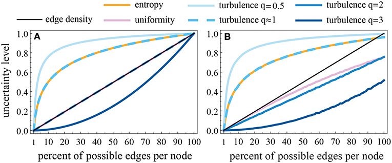
Figure 2. Scaling comparison of the RDMM measures of uncertainty. Each one is normalized onto the [0, 1] range, but has varying sensitivity to differences in the exit probability distributions within that range. Comparison made with 100 nodes and varying the number of edges per node with uniform weight = 1/k (A), or assigning random proportions to each edge (B). Increasing the total number of nodes increases the curvature (deviation away from edge density) of all measures.

Figure 2B shows an example of the values of the measures when the probability weights are heterogeneous. Note that uniformity and turbulence₂ both split further away from normalized edge density as the density of the RDMM increases, but in a different way (this will be important in our empirical analyses later). Also note that even when all edges are present in the network, because the weights are heterogeneous the uncertainly level is <1 because the distribution of edge weights carries information about the system dynamics. None of these scaling patterns is a priori superior, so we evaluate each RDMM measure based on their performance on tests below.

Interestingly, when q = 1 in the turbulence measure it is undefined because the sum of the probabilities is always exactly 1, and hence the minimum and maximum value of the measure are both one. But as q → 1, turbulence becomes equivalent to entropy. The reason for this equivalence is that for small values of x, the Maclaurin series for $ln(1+x)=x-\frac{x^2}{2}+\frac{x^3}{3}-\frac{x^4}{4}+\dots$; and so, when q = 1+10⁻¹⁰ the sum of the node probabilities differ slightly from being exactly 1, and when normalized the scaling of these values is indistinguishable from the scaling of the natural logarithm. For this reason we abandon further analyses of turbulence₁.

2.3. Comparison Measures

We compare our RDMM measures against established measures of uncertainty/complexity that can be directly calculated from the times series. We do not assess other approaches that require an intermediate model, such as neural networks, discrete wavelet transforms, or other types of Markov models. We briefly cover each comparison measure here; further details can be found in the Appendix A and related literature.

First we have three general measures of the variation within the data. (1) Variance is the average of the squared distances from the mean. (2) Volatility is the variance in the log returns, and as such is undefined for many datasets. (3) Jaggedness is the mean of absolute distances among sequential point pairs; this actually measures the monotonicity of the sequence. These three measures are not specifically purported to be measures of uncertainty and are included to ensure that the proposed measures are not merely tracking these basic properties.

We have size more sophisticated measures from the literature that do purport to measure uncertainty: (4) Approximate entropy (ApEn) is the difference in the proportions of windows of length m = 2 and 3 that are within distance r = 0.2σ of each other [5]. (5) Sample entropy (SampEn) is a refinement of ApEn that takes the log ratio of proportions of windows of length m = 2 and 3 that are within distance r = 0.2σ of each other (excluding self-comparisons) [6]. (6) Permutation entropy is the Shannon entropy of the observed proportions of each type of ordinal permutation possible by taking all sets of 5 sequential points [29, 30]. (7) Incremental entropy is the Shannon entropy of a sequence of “words” formed by the magnitude and direction of each incremental pair [8]. (8) The permutation test using non-overlapping windows of length 5 provides a measure via the χ²-test statistic [7]. (9) The runs test determines how well the counts of contiguous chains of values above or below the mean follow a binomial distribution [31, 32]; although usually a test of randomness, its normalized z-score acts as a measure here.

To simply describe the main measures, ApEn/SampEn reflect the lack of short, recurrent, and regular patterns in the time series while permutation and increment entropies describe how locally noisy the system is in different ways. A similarly simple way to describe the proposed RDMM measures is that they track how systematically predictable a sequence is from its previous value. Although none of those summaries do the measures justice, they perhaps provide useful intuitions as we move forward to the data analyses.

3. Data Analysis and Results

Our focus here is demonstrating that the RDMM-based measures are genuine and distinct measures of time series uncertainty with improved accuracy compared to previous measures. We do this by comparing the uncertainty ranks of each measure across a variety of simulated and empirical data sets chosen for their known uncertainty features. We are especially interested in the robustness and consistency properties of these measures across different resolutions of the same data. Partly this is because such binning is required by the RDMM technique and we need to assess the sensitivity to this parameter. Another motivation is because many datasets are digital representations of analog signals, and we wish to ensure our measurements on the coarse-grained data accurately reflects the uncertainty of the underlying data. Using simulated data we can assess whether each measure consistently produces the expected effects. Then, using empirical data we can further assess generality and robustness against irregular noise and systemic change.

3.1. Simulated Data

We generated seven types of time series using functions chosen to systematically explore the measures' relative behaviors. Using ${{N}}_t$ to represent a pull from a random distribution at time t, the functions are (1) a low frequency sine wave: $sin\frac{t}{4\pi }$, (2) a basic sine wave: $sin\frac{t}{\pi }$, (3) a high frequency sine wave: $sin\frac{8t}{\pi }$, (4) random noise: ${{N}}_t$, (5) a random walk: $\sum _{i=1}^t{{N}}_i$, (6) a noisy sine wave: $sin\frac{t}{\pi }+{{N}}_t$, and (7) a randomly walking sine wave: $sin\frac{t}{\pi }+\sum _{i=1}^t{{N}}_i$. Our primary exposition covers one exemplar with T = 1, 200 points using a normal distribution with μ = 0 and σ = 0.4; however, in section 3.1.3 we examine sets of 100 instantiations of longer time series and multiple noise distributions.

For each time series we calculate all measures using equal-width bins numbering from 5–100 in increments of 5. We additionally calculate each non-RDMM measure directly on the original time series (marked as ∞ bins in all plots). Figure 3 shows the values for key measures across binnings for noise (Figure 3A) and the random walk (Figure 3B) to present some recurring relevant highlights regarding the relative behaviors of the different measures for discussion. Below we also discuss the main results from the entire battery of tests; while additional details and figures can be found in Appendix B.

FIGURE 3

Figure 3. The values across resolutions of uncertainty measures applied to random noise (A) and random walk (B) time series using the same instance of ${N}$ for T = 1, 200. Volatility, jaggedness, variance, and the runs test are not shown here to reduce clutter.

Variance and jaggedness have only a small increase over 5–15 bins, but are otherwise insensitive to the binning (flat), volatility cannot be applied to these data because the log returns is undefined when the value is zero, and the runs test (as we used it) shows only the noise series as having non-zero uncertainty (these measures were left off Figure 3). Permutation entropy and the permutation test (red lines) are typically closely linked (redundant), and increment entropy (purple) is also often correlated with them, but sometimes fluctuates independently. However, as can be clearly seen in Figure 3B, 4A,B, all three of these measures reveal increasing uncertainty with increasing resolution on all stochastic series due to a known flaw in how they handle tied values [33, 34]. ApEn and SampEn (green lines) typically have similar patterns with respect to both their magnitude and their sawtooth shape across numbers of bins, but are not completely redundant. One important difference is that ApEn ranks the low-frequency sine wave as more uncertain than both the other deterministic sine waves and the random walk (Appendix B.3.2), while SampEn rates the random walk as equally or slightly less uncertain than the deterministic time series (Figure 4C). Both are inaccurate, but SampEn is revealed to be an improvement over ApEn. In summary, all the previous measures yield at least some counter-intuitive behavior in response the changes in the resolution of the data and/or the ranking of the series' uncertainties.

FIGURE 4

Figure 4. The uncertainty values across resolutions of four selected measures for each of the generated time series using the same instance of ${N}$ for T = 1, 200. Beyond 45 bins, the ranking of the uncertainty by turbulence₂ (D) (and most of the other RDMM measures) stabilizes to what one should expect: the two noise series at top, the deterministic series on the bottom, and the random walks in between. The previous measures each achieve a partially correct ordering (A–C), but also each make different errors.

By contrast, for a sufficiently high number of bins (depending on the number of datapoints, here 45) most of the proposed RDMM measures rank the simulated time series as expected: the two noise series at top, the deterministic series on the bottom, and the random walks in between (turbulence₂ shown in Figure 4D other measure's plots are available in Appendix B.3.2). Some RDMM measures are better than others. For example, turbulence₃ can be eliminated from consideration because it just behaves as a dampened turbulence₂; having both is redundant and turbulence₂'s greater sensitivity makes examining results easier. Turbulence_0.5 and entropy yield prolonged increasing uncertainty with increasing bins for the random walk and walking sine wave time series, although it levels off after 50 60 bins. Turbulence_0.5 is more extreme than entropy, and is the only RDMM measure that gets the uncertainty ranking incorrect (putting the random walk above noise after 75 bins). Turbulence_0.5 and entropy can be tentatively eliminated as viable measures of uncertainty, but we continue to include them in the analysis. Uniformity and edge density are also similar enough to be considered redundant, and edge density was merely included as a control measure, thus making uniformity less appealing as a measure of uncertainty because it is insufficiently sensitive to the edge weights.

Many of the RDMM results just described are ramifications of the differences in network density scaling presented in section 2.2. For a given dataset, as the number of bins increases, the density of the Markov model typically decreases. As the density decreases, the uncertainty would intuitively tend to decrease, but it depends on how low vs. high probability edges are factored into the measure. Turbulence_0.5 and (evidently) entropy factor low-weighted edges too strongly into the uncertainty calculation; thus a random walk appears highly deterministic with low numbers of bins, but comes out as increasingly random with higher numbers of bins. We continue the analysis and evaluation below, but these results already demonstrate that the RDMM approach (and turbulence₂ in particular) can distinguish and accurately measure the uncertainty of time series dynamics in a way that previous methods cannot.

3.1.1. Monotonicity Analysis

An analysis of the average monotonicity (mean over the datasets of the jaggedness of the measures across bins – Appendix Table B.2 and Figure B.8) reveals that (after variance) the RDMM measures are generally the most consistent, which is an indicator of their robustness to changes in resolution. In some cases (variance, edge density, turbulence₃) the high robustness is really reflecting a general lack of sufficient sensitivity, while in others (permutation and increment entropies) the lack of sensitivity depends on the dataset or reflects an artifact of the measures. ApEn and SampEn do the worst here. Although edge density is extremely close to monotonically decreasing with increasing number of bins, and the RDMM measures typically have a smoother response curve than previous measures, this isn't enough to confirm or deny that the RDMM measures are monotonically increasing with increasing actual uncertainty because of the sensitivity of all measures to where exactly the bins cut the data. For example, while the measured monotonicity of turbulence₂ is mediocre, this fails to reflect that consistently across datasets there is a clear trend toward convergence as the number of bins increases.

3.1.2. Reversing the Time Series

Running a time series in reverse will have an effect on its predictability only under certain concepts of uncertainty; e.g., when applied to text, music, or animal trajectories. Among time series uncertainty measures, only the proposed RDMM ones are properly sensitive to the direction (although permutation-based methods are also effected by the order due to the aforementioned tie-breaking flaw). RDMM measures are direction-sensitive because the transition probabilities of the generated Markov model will change, as can be clearly seen in the following simplified example. Consider the following sequence of values:

$1\to 1\to 2\to 2\to 3\to 3\to 4\to 5\to 5\to 5$

This series produces distinct Markov models when encoded forward and backward as can be seen in Figure 5. It is worth mentioning here because it signals a conceptual benefit as well as an accuracy benefit in using RDMMs to understand and measure time series dynamics, although we found only small differences in the uncertainty values for the datasets analyzed.

FIGURE 5

Figure 5. Example Markov model demonstrating the difference in edge weights between running the data forward (top) and in reverse (bottom).

3.1.3. Broader Robustness Results

Although the limitation to 1,200 points reflects the reality of many empirical time series, and exceeds the recommended minimum points for previous measures of uncertainty [35–37], in a further robustness test we analyze time series with 10,001 points using 100 realizations of two kinds of random seeds for the noise sequence. We also test the effects of the distribution shape by including three standard deviation values for the Normal distribution (σ = {0.4, 0.8, 1.2}) as well as a Uniform distribution with endpoints at {(−0.4, 0.4), (−0.8, 0.8), (−1.2, 1.2)}. The deterministic series are (obviously) unaffected by changes in the distribution parameter and left out of this analysis. Several measures have already been eliminated from consideration, and although their results appear in the Appendix, we focus on the main results of the remaining measures here.

On the random noise series, all measures produce similar trajectories with slight variation using the Normal distribution (Figure 6A), but largely consistent values at each resolution for all realizations of uniform noise (Figure 6B). Note that for the random noise series, no measure is systematically affected by changing the distribution parameters; widening either distribution produces no measurable difference in uncertainty (figures available in Appendix B.8). However, there is a marked difference in the behavior of the RDMM measures between Normal and Uniform noise. Specifically, the RDMM measures (but not the previous measures) report greater uncertainty for the Uniform distribution across all resolutions. This is because the normal distribution produces a pattern in the exit transitions of the induced Markov model, with more edges and stronger weights in the center and fewer/weaker links at the periphery, but the uniform distribution (obviously) produces a more uniform Markov model. This is exactly the sense of uncertainty we are aiming to measure with this technique: the existence of a (potentially stochastic) pattern in the time series that yields information about the generating mechanism. The ability of the RDMM measures, and the inability of the non-RDMM measures, to capture this difference is a clear benefit of the proposed technique.

FIGURE 6

Figure 6. The uncertainty values across resolutions of selected measures applied to the random noise series using 100 distinct instances of Normally (A) and Uniformly (B) distributed noise for T = 10, 001.

For the random walk, none of the measures report systemically higher or lower uncertainty values across increasing parameter values or between normal and uniform distributions as shown in Figure 7. Because there is no underlying pattern in the random walk, the resulting trajectory of accumulated noise does not vary (systematically) depending on the type of noise. The characteristic behavior of random walks does not depend on the particular kind of (symmetric) random noise distribution that generates them.

FIGURE 7

Figure 7. The uncertainty values across resolutions of selected measures applied to the random walk series using 100 distinct instances of Normally (A) and Uniformly (B) distributed noise for T = 10, 001.

Figure 8 summarizes the results of normally vs. uniformly distributed noise for the noisy sine wave and random walking sine wave. The pattern of results across bins for the noisy sine wave are similar to noise in Figure 6, but there are two key differences. First, increasing noise yields an increase in the uncertainly level for all measures, and this effect is stronger for uniform noise. Second, the discrepancy between Normal and Uniform noise is much smaller due to a reduced effect from Uniform noise. This is because the effect of a little noise is small compared to the curvature of the sine wave, so there is still a visible sine wave moving up and down, and sine waves are predictable. Increasing the noise level drowns out the sine wave pattern, so it looks more like just noise, and the uncertainty values of all measures reflect this.

FIGURE 8

Figure 8. The uncertainty value of the noisy sine wave and random walking sine wave by selected measures at 50 bins for 100 realizations of Normally and Uniformly distributed noise across dispersion values.

The random walking sine wave provides an interesting mix of the random walk and noisy sine wave. In this case increasing the dispersion of the noise has the effect of reducing the uncertainty for both normal and uniform distributions (though slightly more pronounced for uniform noise). This is also caused by the underlying sine wave providing a recognizable pattern. However, in this case, as the noise increases, the accumulated values look less like a noisy sine wave and more like a random walk; and random walks have lower uncertainty than noisy sine waves, so the net effect of increased noise is reduced uncertainty. This is true for the RDMM measures as well as SampEn, but not for permutation entropy.

These tests show that the RDMM measure's ability to accurately rank the uncertainty of each dataset is (1) robust against the time series length and (2) largely invariant to any particular draw from the random distribution. We find that in some cases uniform noise does indeed yield less predictable series than normally distributed noise, but this is effect is only picked up by RDMM measures. We also find that increased random dispersion relative to the wave amplitude reduces the information provided by the wave's contribution to the dynamics in intuitive ways and this information content cannot be detected by permutation entropy. We can conclude that the RDMM approach can reliably capture (and can distinguish) overall dynamical patterns such as oscillation, continuity, noise type, and various combinations thereof rather than merely pick up idiosyncratic variations of particular datasets. We have demonstrated several benefits of the RDMM approach based on our analyses of generated data, now we continue to empirical datasets with intuitive uncertainty rankings but unknown functional forms.

3.2. Weather Data

Weather prediction is clearly important, and hidden Markov models (HMM) have long been useful for this task [38–41]. The point of the HMM approach is that there is an underlying (hidden) causal mechanism with parameters that can be reverse-engineered from the observed data and then used to make near-term predictions. Our technique is not being proposed for making predictions, it instead describes the observed dynamics in a way that facilitates new measures of system uncertainty. As mentioned above, one way to think about it is that uncertainty measures on the RDMM inform us of how complicated the HMM (or other model) would need to be to capture the dynamics in a certain weather system.

To test our measures of uncertainty we analyze daily temperature and precipitation data for New York, NY; San Diego, CA; Phoenix, AZ; and Miami, FL using NOAA data from Jan 1, 2010 to Dec 31, 2016 (T = 2557) from [42] (and available upon request). Plots of the first half of each time series appear in Figure 9 to foster the readers' intuitions regarding their relative uncertainty levels. These cities were chosen because of their distinct mixes of temperature and precipitation patterns: New York and Phoenix have similar temperature variations, but very different precipitation levels whereas Miami and San Diego have similar temperatures and very different rain patterns. On the other hand, San Diego and Phoenix have similar rain patterns, as do New York and Miami. Thus, these four cities together occupy each square of a 2 × 2 grid of low and high temperature fluctuations and precipitation amounts. Because of these relationships we can establish an intuitive ranking of the uncertainty of weather in these cities. In order from most predictable to most uncertain are (1) San Diego, (2) Phoenix/Miami, and (3) New York. Phoenix and Miami tie for second in our intuitive ranking because the two cities are trading off variation in one time series with the other; the resulting ranking will depend on whether precipitation or temperature is more uncertain. We test how each measure performs in matching our expectation, as well as their sensitivity to binning.

FIGURE 9

Figure 9. Plots of the first half of the temperature and precipitation data for all four cities. Plots of the full time series appear in Appendix C.

One reason we chose weather data is to demonstrate the shared binning adjustments necessary to ensure that the uncertainty results can be compared on the same scale across datasets. Using shared binning means the min and max across all four cities are used to determine the bins for all four analyses. Without shared binning, independent normalization to the observed ranges within each city would make (among other irregularities) all temperature series appear similar and likely yield similar uncertainty values despite their clear differences in magnitudes.

For RDMM entropy the shared normalization is a straightforward replacement of n (number of nodes; i.e., observed states) with B (the number of bins). Re-normalizing of edge density and turbulence requires changing 1/n in the original formations to n/B²: thus shared-bin turbulence becomes

$\begin{array}{cc}\frac{\frac{1}{B^2}{\displaystyle {\sum }_{s_i\in S}{\kappa }_i}-\frac{n}{B^2}}{{\left(\frac{n}{B^2}\right)}^{2-q}-\frac{n}{B^2}}=\frac{{\displaystyle {\sum }_{s_i\in S}{\kappa }_i}-n}{n{\left(\frac{n}{B^2}\right)}^{1-q}-n}.& (10)\end{array}$

For uniformity it is necessary to convert the n × n adjacency matrix into a B×B matrix by padding the difference with identity matrix entries (s_i ∉ S → p_ii = 1, p_ij = 0). For all RDMM measures, in order to reach maximum uncertainty under a shared binning scheme, a series would need a uniform distribution of edge weights across all bins.

We find that temperature (which looks like a noisy sine wave but yields results closer to the random walk) is rated as more uncertain than precipitation by all measures for most bin values. For precipitation, the previous measures pair NY≈Mi and SD≈Ph (see sample entropy in Figure 10A) while the RDMM measures consistently rank precipitation uncertainty as Mi>NY>SD>Ph (see turbulence₂ in Figure 10B). This demonstrates that the RDMM measures are picking up on differences in the magnitudes and seasonality of the dynamics that the previous measures can not capture. Furthermore, the ranking of temperature uncertainty reported by the RDMM measures consistently matches the intuitively correct order (NY>Ph>Mi>SD), while the non-RDMM measures (except for increment entropy) are neither consistent nor intuitively correct. Thus, for both precipitation and temperature we achieve better results using the RDMM measures than previous measures.

FIGURE 10

Figure 10. Uncertainty levels across numbers of bins for SampEn (A) and turbulence₂ (B). The rankings of the RDMM measures are both consistent and intuitively correct while the previous measures fail to reflect the expected relative levels of time series complexity.

One point of this empirical data analysis was to introduce the shared binning modification. We saw that when comparing datasets of the same kind of data, the binning should be done using the [min, max] range of the combined data so that the resulting Markov model states represent the same interval of values across analyses. From analyzing the weather data we find that some dynamical patterns' uncertainty can be captured by most measures, but there are important differences in the size and frequency of changes that only the RDMM measures reveal.

3.3. Exchange Rates

We next analyze the value of the United States Dollar (USD), Japanese Yen (JPY), and Russian Ruble (RUB) in terms of Euros using references rates from Jan 1, 2000 to Dec 31, 2016 (T = 4351) collected from D'ITALIA [43] (shown in Figure 11 and available upon request). The three currencies' uncertainties have the same rank by all measures: JPY>USD>RUB. Because these exchange rates are in terms of Euros, the Ruble's lower uncertainty implies that it the depends the most on (and is therefore most highly correlated with) the Euro, and the Dollar more so than the Yen. It is possible to standardize the three time series (by, for example, subtracting the mean and dividing by the standard deviation) and/or filter out the shared variations, but for our current purposes it is acceptable to provide a Euro-centric analysis because such an analysis suffices to compare the relative uncertainty of the three referenced currencies. That is, the relative uncertainty measurements are invariant to standardization manipulations.

FIGURE 11

Figure 11. Time series data of the exchange rates of the Japanese Yen (JPY), Russian Ruble (RUB), and United States Dollar (USD) in terms of Euros across the period of analysis.

As is typical of exchange rate time series, ours look similar to random walks, and as we saw in section 3.1 these kinds of patterns are very predictable in the sense that most daily variations are small compared to the full historic range. The result is therefore low uncertainty values for many RDMM measures (as well as ApEn and SampEn), but high uncertainty for local-variation detecting permutation and increment entropies. On this data we see that coarse-graining the data, even a little bit, significantly affects these latter measures because they reflect short-term fluctuations in the data. Greater resolution exposes more local noise and these measures' values increase toward the unbinned limit near complete uncertainty for all currencies.

That is to be expected – it is more interesting to note that the RDMM measures level off to intermediate values, and to distinct values for each currency, successfully capturing the distinct information contained within them. Note that turbulence₂ (up to now the best-performing measure) yields very similar values for all three currencies; in fact, more similar than any other (binned) measure. So although the Markov model of the revealed dynamics seems to tease out the nuanced differences in their behaviors, turbulence₂ consistently reports a tiny difference in the uncertainty of those behaviors. One way to interpret this results is that, despite the RDMM capturing three currencies' behavior as distinct, the measure gets it right because they actually do have similar uncertainty levels. That is a plausible conclusion, especially when looking at the similarity of their time series plots in Figure 11; however, one may instead conclude that RDMM measures, and turbulence₂ in particular, may be bad at reflecting differences among random walk-like dynamics. Considering that the uncertainty values are also very similar according to SampEn, unbinned permutation/increment entropy, and the other RDMM measures, we tend toward supporting turbulence₂'s evaluation: the Yen is the most uncertain, and the Ruble the least uncertain, but the difference in uncertainty is minute.

3.3.1 Combined Exchange Rates Analysis

Because all three series are in terms of the Euro, there is shared information in their dynamics. One of the advantages of the RDMM encoding is that it can capture multiple dimensions simultaneously, and we demonstrate that capability here by analyzing all three exchange rate datasets together in one RDMM. Because we only need a node for those combinations of values that actually occur in the combined time series, this method suffers less from the exponential expansion of the phase space volume with each added dimension. There are never more nodes in the RDMM than points in the data, and with binning there are (if the model is going to be useful) many fewer nodes than datapoints regardless of the dimensionality.

Compared to the one-dimensional case in which nearly 100% of the bins become nodes, raising the dimension greatly increases the number of bins (B³ in this case). Because there are only 4,351 data points, as the number of bins increases, most of them are empty (see Table 1). However, because the three series are correlated, most of the B³ possible combinations of the variables are never seen, and so those empty bins do not get represented as a node of the RDMM. So although we find low proportions of bins being used even for lower numbers of bins, The number of new nodes being created decreases as the number of bins increase. The three series are not independently random, and the amount of their joint information can be read from the structure of the generated RDMM. Specifically, the uncertainty changes of the combined vs individual RDMMs provide insights similar to mutual, conditional, and transfer entropy on the causal influence/interactions of time series [44, 45].

TABLE 1

Table 1. Top table reports the proportion of bins used for each number of bins for each exchange rate time series.

The next point is about how the measures of uncertainty differ with a multidimensional analysis. For the non-RDMM measures we can only calculate some aggregate of the individual measures (e.g., mean is used here). The uncertainty values still change in our analysis because although these measures were applied to each series independently, we applied them to the data binned according to the multidimensional binning. That rebinning raises the uncertainty reported by these measures, but the RDMM measures tell us that fusing the correlated time series makes their combined uncertainty less than their parts, even when adjusting for the much larger number of bins (see Figure 12). This is just as we should expect. Although for large numbers of bins there are too few datapoints to provide high-confidence measures of uncertainty, the observed reduced uncertainty even at lower bins reflects how the RDMM technique captures the shared information across the distinct time series to correctly report that analyzing multiple exchange rate series together reduces our uncertainty of how the exchange rate market fluctuates over time. Another viable interpretation of this result is that the reduced RDMM uncertainly is being driven entirely by the reduced density of the generated RDMM. We discuss this later possibility and need for further normalization in the conclusions section.

FIGURE 12

Figure 12. Uncertainty levels across numbers for selected measures for both the Russian Ruble and the three-dimensional time-series of the three exchange rate combined.

4. Conclusions

Representing a time series as a Markov model of the phase space fosters the analysis of the system's uncertainty in a novel way. We explore three new measures of uncertainty based on this RDMM and compare them to existing measures of time series uncertainty. Our results demonstrate that the proposed measures capture distinct sources of uncertainty compared to previous measures, such as variations in the magnitude of changes and the tradeoff between noise and an underlying signal, as well as provide improved accuracy of relative uncertainty values.

One surprising result is that Shannon entropy on an RDMM has undesirable properties for a measure of system uncertainty; specifically, increasing uncertainty values across increasing resolution/information in many cases. This effect is generated by the concave sensitivity profile of the measure shown in Figure 2 that puts too much weight on low-probability edges. Uniformity's linear profile has superior features, but the measure lacks sufficient sensitivity to edge weights. Although turbulence with q = 2 comes out ahead overall on our tests, it is not without some worries. Low levels of uncertainty for random walks implies that these measures do bot pick up on the randomness because this kind of accumulative randomness is small when considered as a Markov process (as well as by ApEn and SampEn).

Considering the results, if one needs to select a single measure of time series uncertainty, then turbulence₂ is the best choice However, as we demonstrated, all the RDMM measures perform well in some tests, and scale differently on different kinds of dynamics. Similarly we showed that the RDMM measures, by analyzing the Markov model encoding all of the observed dynamics holistically, capture distinct features of the dynamics compared to previous measures that examine local time windows. Even variance, jaggedness, and volatility (where applicable) provide information on different senses of uncertainty. For this reason one may consider an ensemble approach that combines multiple measures to reflect multiple senses of uncertainty in an uncertainty profile. Although one could include all the measures, based on the correlations, redundancies, and accuracies found in our analysis, including SampEn, permutation entropy, and turbulence₂ may be sufficient. Such an ensemble approach may provide better classification performance for machine learning applications because it can potentially discriminate among multiple kinds of uncertainty.

The non-RDMM measures of complexity each include parameters (window size, threshold, etc.) that strongly effect the results but are usually just set by heuristics. The only parameter for RDMM measures is binning (and q, but we've already explored its effect on turbulence). We showed how one can specify the maximum number of bins supported by a series of length T using $B_m=\lfloor \sqrt[2D]{T-1}\rfloor$ (for D-dimensional data), and we explained that having too few points depresses the uncertainty measures values because the Markov model becomes too sparse (which is similar to being more deterministic and hence less uncertain). However, a better binning method would adapt to an ideal number of nodes (rather than bins) and depend on a desired number of observations per node, or a desired confidence level across the model. Our presentation using simple binning and a heuristic for the number of bins parallels how previous methods set standards for a minimum (typically 100) and recommended (such as 900) number of consecutive points [30, 35–37]. Having insufficient data depresses their reported values as well. Future work will explore (a) data-sensitive normalization schemes (b) multinomial confidence levels for nodes and (c) more sophisticated binning methods (equal-contents bins, agglomerative binning, clustering, etc.) in order to best handle the data/resolution tradeoff.

One advantage of the RDMM approach is the ability to analyze multi-dimensional time series where the curse of dimensionality is softened because the RDMM only includes nodes for observed combinations of binned values. This is especially valuable for fusing categorical and numerical temporal data. Another advantage is that (in some cases) one can combine multiple independent trials into a unified RDMM; even if the length of each series is short, the combined sequences can fill out the details of the dynamical process. Furthermore, the descriptive Markov models can be used to measure time series similarity for unsupervised classification of behavior types [9] while offering an intuitive window into the dynamics rather than a black box.

Measures of uncertainty have been usefully deployed on cardiac, neurological, and financial time series already (e.g., using time-windowed assessments of changes in uncertainty for event detection). Here we focused on system-wide uncertainty to demonstrate that RDMMs robustly capture distinct features of dynamical patterns to more accurately capture their uncertainty levels. Future work will, aside from the above-mentioned methodological innovations, also include applications utilizing these measures to make a valuable contribution to assessments of system uncertainty for risk management and event prediction as well as behavior classification. For now, what we have accomplished is a contribution to a body of measures to evaluate time series data utilizing a novel form of Markov model that outperform previous measures in many ways.

Author Contributions

AaB and AI designed the research. AaB performed the research. AaB and AdB collected and analyzed data. AaB wrote the paper.

Funding

This research was supported by AMED's Brain/MINDS project under Grant Number JP15km0908001.

Conflict of Interest Statement

This research may lead to the development of products which may be licensed to Rikaenalysis Corporation (a RIKEN Venture), in which AI is the president and CEO and AaB is CSO.

The remaining author declares that the research was conducted in the absence of any commercial or financial relationships that could be construed as a potential conflict of interest.

Supplementary Material

The Supplementary Material for this article can be found online at: https://www.frontiersin.org/articles/10.3389/fams.2019.00007/full#supplementary-material

References

1. Lake DE, Moorman JR. Accurate estimation of entropy in very short physiological time series: the problem of atrial fibrillation detection in implanted ventricular devices. Am J Physiol Heart Circ Physiol. (2011) 300:H319–25. doi: 10.1152/ajpheart.00561.2010

PubMed Abstract | CrossRef Full Text | Google Scholar

2. Cao Y, Tung Ww, Gao J, Protopopescu VA, Hively LM. Detecting dynamical changes in time series using the permutation entropy. Phys Rev E. (2004) 70:046217. doi: 10.1103/PhysRevE.70.046217

PubMed Abstract | CrossRef Full Text | Google Scholar

3. Kannathal N, Choo ML, Acharya UR, Sadasivan P. Entropies for detection of epilepsy in EEG. Comput Methods Programs Biomed. (2005) 80:187–94. doi: 10.1016/j.cmpb.2005.06.012

PubMed Abstract | CrossRef Full Text | Google Scholar

4. Molgedey L, Ebeling W. Local order, entropy and predictability of financial time series. Eur Phys J B-Condensed Matter Complex Syst. (2000) 15:733–7. doi: 10.1007/s100510051178

CrossRef Full Text | Google Scholar

5. Pincus SM. Approximate entropy as a measure of system complexity. Proc Natl Acad Sci USA. (1991) 88:2297–301. doi: 10.1073/pnas.88.6.2297

PubMed Abstract | CrossRef Full Text | Google Scholar

6. Richman JS, Moorman JR. Physiological time-series analysis using approximate entropy and sample entropy. Am J Physiol Heart Circ Physiol. (2000) 278:H2039–49. doi: 10.1152/ajpheart.2000.278.6.H2039

PubMed Abstract | CrossRef Full Text | Google Scholar

7. Knuth DE. The Art of Computer Programming, Vol. 2, 3rd ed., Seminumerical Algorithms. Boston, MA: Addison-Wesley Longman Publishing Co., Inc. (1997).

Google Scholar

8. Liu X, Jiang A, Xu N, Xue J. Increment entropy as a measure of complexity for time series. Entropy (2016) 18:22. doi: 10.3390/e18010022

CrossRef Full Text | Google Scholar

9. Ghassempour S, Girosi F, Maeder A. Clustering multivariate time series using hidden Markov models. Int J Environ Res Publ Health (2014) 11:2741–63. doi: 10.3390/ijerph110302741

PubMed Abstract | CrossRef Full Text | Google Scholar

10. Vidyasagar M. Hidden Markov Processes: Theory and Applications to Biology. Princeton, NJ: Princeton University Press (2014).

Google Scholar

11. Ye N. A markov chain model of temporal behavior for anomaly detection. In: Proceedings of the 2000 IEEE Systems, Man, and Cybernetics Information Assurance and Security Workshop. Vol. 166. West Point, NY (2000). p. 169.

Google Scholar

12. Rains EK, Andersen HC. A Bayesian method for construction of Markov models to describe dynamics on various time-scales. J Chem Phys. (2010) 133:144113. doi: 10.1063/1.3496438

PubMed Abstract | CrossRef Full Text | Google Scholar

13. Rabiner LR. A tutorial on hidden Markov models and selected applications in speech recognition. Proce IEEE. (1989) 77:257–86. doi: 10.1109/5.18626

CrossRef Full Text | Google Scholar

14. Fine S, Singer Y, Tishby N. The hierarchical hidden Markov model: analysis and applications. Mach Learn. (1998) 32:41–62. doi: 10.1023/A:1007469218079

CrossRef Full Text | Google Scholar

15. Shalizi CR, Shalizi KL. Blind Construction of Optimal Nonlinear Recursive Predictors for Discrete Sequences (2004). Available online at: arxiv.org/abs/cs/0406011v1

16. Zucchini W, MacDonald IL, Langrock R. Hidden Markov Models for Time Series: An Introduction Using R. Vol. 150. Boca Raton, FL: CRC Press (2016).

Google Scholar

17. Tauchen G. Finite state markov-chain approximations to univariate and vector autoregressions. Econ Lett. (1986) 20:177–81. doi: 10.1016/0165-1765(86)90168-0

CrossRef Full Text | Google Scholar

18. Page L, Brin S, Motwani R, Winograd T. The PageRank Citation Ranking: Bringing Order to the Web. Stanford InfoLab (1999). 1999-66. Previous number = SIDL-WP-1999-0120. Available online at: http://ilpubs.stanford.edu:8090/422/.

Google Scholar

19. Singhal N, Pande VS. Error analysis and efficient sampling in Markovian state models for molecular dynamics. J Chem Phys. (2005) 123:204909. doi: 10.1063/1.2116947

PubMed Abstract | CrossRef Full Text | Google Scholar

20. Donner RV, Zou Y, Donges JF, Marwan N, Kurths J. Ambiguities in recurrence-based complex network representations of time series. Phys Rev E. (2010) 81:015101(R). doi: 10.1103/PhysRevE.81.015101

PubMed Abstract | CrossRef Full Text | Google Scholar

21. Boccaletti S, Latora V, Moreno Y, Chavez M, Hwang DU. Complex networks: structure and dynamics. Phys Rep. (2006) 424:175–308. doi: 10.1016/j.physrep.2005.10.009

CrossRef Full Text | Google Scholar

22. Zhang J, Small M. Complex network from pseudoperiodic time series: topology versus dynamics. Phys Rev Lett. (2006) 96:238701. doi: 10.1103/PhysRevLett.96.238701

PubMed Abstract | CrossRef Full Text | Google Scholar

23. Donner RV, Zou Y, Donges JF, Marwan N, Kurths J. Recurrence Networks-A Novel Paradigm for Nonlinear Time Series Analysis (20090. Available online at: arxiv.org/abs/0908.3447.

24. Shannon CE, Weaver W. The Mathematical Theory of Communication. Urbana, IL: University of Illinois Press (1971).

PubMed Abstract | Google Scholar

25. Barrat A, Barthelemy M, Pastor-Satorras R, Vespignani A. The architecture of complex weighted networks. Proc Natl Acad Sci USA. (2004) 101:3747–52. doi: 10.1073/pnas.0400087101

PubMed Abstract | CrossRef Full Text | Google Scholar

26. Opsahl T, Agneessens F, Skvoretz J. Node centrality in weighted networks: Generalizing degree and shortest paths. Soc Netw. (2010) 32:245–51. doi: 10.1016/j.socnet.2010.03.006

CrossRef Full Text | Google Scholar

27. Simpson EH. Measurement of diversity. Nature (1949) 163:688. doi: 10.1038/163688a0

CrossRef Full Text | Google Scholar

28. Laakso M, Taagepera R. Effective number of parties: a measure with application to west europe. Comp Polit Stud. (1979) 12:3–27. doi: 10.1177/001041407901200101

CrossRef Full Text | Google Scholar

29. Bandt C, Pompe B. Permutation entropy: a natural complexity measure for time series. Phys Rev Lett. (2002) 88:174102. doi: 10.1103/PhysRevLett.88.174102

PubMed Abstract | CrossRef Full Text | Google Scholar

30. Riedl M, Müller A, Wessel N. Practical considerations of permutation entropy. Eur Phys J Spec Top. (2013) 222:249–62. doi: 10.1140/epjst/e2013-01862-7

CrossRef Full Text | Google Scholar

31. Bradley JVJV. Distribution-Free Statistical Tests. Technical Report (1968).

32. NIST. NIST/SEMATECH e-Handbook of Statistical Methods (2012). Available online at: http://www.itl.nist.gov/div898/handbook/eda/section3/eda35d.htm.

33. Eudey TL, Kerr JD, Trumbo BE. Using R to simulate permutation distributions for some elementary experimental designs. J Stat Educ. (2010) 18:1–30. doi: 10.1080/10691898.2010.11889473

CrossRef Full Text | Google Scholar

34. Zunino L, Olivares F, Scholkmann F, Rosso OA. Permutation entropy based time series analysis: equalities in the input signal can lead to false conclusions. Phys Lett A. (2017) 381:1883–92. doi: 10.1016/j.physleta.2017.03.052

CrossRef Full Text | Google Scholar

35. Pincus SM, Goldberger AL. Physiological time-series analysis: what does regularity quantify? Am J Physiol Heart Circ Physiol. (1994) 266:H1643–56. doi: 10.1152/ajpheart.1994.266.4.H1643

PubMed Abstract | CrossRef Full Text | Google Scholar

36. Pincus S. Approximate entropy (ApEn) as a complexity measure. Chaos (1995) 5:110–7. doi: 10.1063/1.166092

PubMed Abstract | CrossRef Full Text | Google Scholar

37. Costa M, Goldberger AL, Peng CK. Multiscale entropy analysis of biological signals. Phys Rev E. (2005) 71:021906. doi: 10.1103/PhysRevE.71.021906

PubMed Abstract | CrossRef Full Text | Google Scholar

38. Gabriel K, Neumann J. A Markov chain model for daily rainfall occurrence at Tel Aviv. Q J R Meteorol Soc. (1962) 88:90–5. doi: 10.1002/qj.49708837511

CrossRef Full Text | Google Scholar

39. Caskey Jr JE. A Markov chain model for the probability of precipitation occurrence in intervals of various length. Mon Weather Rev. (1963) 91:298–301. doi: 10.1175/1520-0493(1963)091<0298:AMCMFT>2.3.CO;2

CrossRef Full Text | Google Scholar

40. Haan C, Allen D, Street J. A Markov chain model of daily rainfall. Water Resour Res. (1976) 12:443–9. doi: 10.1029/WR012i003p00443

CrossRef Full Text | Google Scholar

41. Alasseur C, Husson L, Pérez-Fontán F. Simulation of Rain Events Time Series with Markov Model. In: Personal, Indoor and Mobile Radio Communications, 2004. PIMRC 2004. 15th IEEE International Symposium. Vol. 4, Barcelona (2004). p. 2801–5.

Google Scholar

42. NOAA. Daily Summries (Temperature and Precipitation), January 1, 2010– December 31, 2016 (2017).

43. D'ITALIA B. Reference Exchange Rates Against Euro From 01/01/2000 to 31/12/2016 (2017). Available online at: http://cambi.bancaditalia.it/cambi/cambi.do?lingua=en&to=cambiSSGForm.

44. Schreiber T. Measuring information transfer. Phys Rev Lett. (2000) 85:461. doi: 10.1103/PhysRevLett.85.461

PubMed Abstract | CrossRef Full Text | Google Scholar

45. Hlaváčková-Schindler K, Paluš M, Vejmelka M, Bhattacharya J. Causality detection based on information-theoretic approaches in time series analysis. Phys Rep. (2007) 441:1–46. doi: 10.1016/j.physrep.2006.12.004

CrossRef Full Text | Google Scholar