Derandomizing Compressed Sensing With Combinatorial Design

1. Introduction and Main Results

1.1. Motivation

Compressed sensing is the art of effectively reconstructing structured signals from substantially fewer measurements than would naively be required for standard techniques like least squares. Although not entirely novel, rigorous treatments of this observation [1, 2] spurred considerable scientific attention from 2006 on (see e.g., [3, 4]) and references therein. While deterministic results do exist, the strongest theoretic reconstruction guarantees still rely on randomness. Each measurement corresponds to the observed inner product of the unknown vector, with a vector chosen randomly from a fixed measurement ensemble. Broadly, these ensembles can be grouped into two families:

(i) Generic measurements such as independent Gaussian, or Bernoulli vectors. Such an abundance of randomness allows establishing very strong results by following comparatively simple and instructive proof techniques. The downside is that concrete implementations do require a lot of randomness. In fact, they might be too random to be useful for certain applications.

(ii) Structured measurements such as random rows of a Fourier, or Hadamard matrix. In contrast to generic measurements, these feature a lot of structure that is geared toward applications. Moreover, selecting random rows from a fixed matrix does require very little randomness. For example, log₂(n) random bits are sufficient to select a row of the DFT uniformly at random. In contrast, generating an i.i.d. Bernoulli vector would consume n bits of randomness. Structure and comparatively little randomness have a downside, though. Theoretic convergence guarantees tend to be weaker than their generic counterparts. It should also not come as a surprise that the necessary proof techniques become considerably more involved.

Typically, results for type (i) precede the results for type (ii). Phase retrieval via PhaseLift is a concrete example for such a development. Generic convergence guarantees [5, 6] preceded (partially) de-randomized results [7, 8]. Compressed sensing is special in this regard. The two seminal works [1, 2] from 2006 provided both results almost simultaneously. This had an interesting consequence. Despite considerable effort, to date there still seems to be a gap between both proof techniques.

Here, we try to close this gap by applying a method that is very well established in theoretical computer science: partial derandomization. We start with a proof technique of type (i) and considerably reduce the amount of randomness required for it to work. While doing so, we keep careful track of the amount of randomness that is still necessary. Finally, we replace the original (generic) random measurements with pseudo-random ones that mimic them in a sufficiently accurate fashion. Our results highlight that this technique almost allows bridging the gap between existing proof techniques for generic and structured measurements: the results are still strong but require slightly more randomness than choosing vectors uniformly from a bounded orthogonal system, such as Fourier or Hadamard vectors.

There is also a didactic angle to this work: within the realm of signal processing, partial-derandomization techniques have been successfully applied to matrix reconstruction [8, 9] and phase retrieval via PhaseLift [7, 10, 11]. Although similar in spirit, the more involved nature of these problems may obscure the key ideas, intuition and tricks behind such an approach. However, the same techniques have not yet been applied to the original problem of compressed sensing. Here, we fill this gap and, in doing so, provide an introduction to partial derandomization techniques by example. To preserve this didactic angle, we try to keep the presentation as simple and self-contained as possible.

Finally, one may argue that compressed sensing has not fully lived up to the high expectations of the community yet (see e.g., Tropp [12]). Arguably, one of the most glaring problems for applications is the requirement of choosing individual measurements at random¹. While we are not able to fully overcome this drawback here, the methods described in this work do limit the amount of randomness required to generate individual structured measurements. We believe that this may help to reduce the discrepancy between “what can be proved” and “what can be done” in a variety of concrete applications.

1.2. Preliminaries on Compressed Sensing

Compressed sensing aims at reconstructing s-sparse vectors x ∈ ℂⁿ from m ≪ n linear measurements:

$\begin{array}{l}\text{y}=\text{A}\text{x}\in {ℂ}^m.\end{array}$

Since m ≪ n, the matrix A is singular and there are infinitely many solutions to this equation. A convex penalizing function is used to promote sparsity among these solutions. Typically, this penalizing function is the ℓ₁-norm ${\Vert \text{z}\Vert }_{{\ell }_1}=\sum _{i=1}^n|z_i|$:

$\begin{array}{ll}{\displaystyle \underset{\text{z}\in {ℂ}^n}{\text{minimize}}}& {\Vert \text{z}\Vert }_{{\ell }_1}\\ \text{subject to}& \text{A}\text{z}=\text{y}& (1)\end{array}$

Strong mathematical proofs for correct recovery have been established. By and large, these statements require randomness in the sense that each row ${\text{a}}_i\in {ℂ}^n$ of A is an independent copy of a random vector a ∈ ℝⁿ. Prominent examples include

(1) m = Cs log(n/s) standard complex Gaussian measurements: ${\text{a}}_g~{N}(0,\mathbb{\text{I}}/\sqrt{2})+i{N}(0,\mathbb{\text{I}}/\sqrt{2})$,

(2) m = Cs log(n/s) signed Bernoulli (Rademacher) measurements: ${\text{a}}_{sb}~{\left\{\pm 1\right\}}^n$,

(3) m = Cs log⁴(n) random rows of a DFT matrix: a_f ~ {f₁, …, f_n},

(4) for n = 2^d: m = Cs log⁴(n) random rows of a Hadamard matrix: a_h ~ {h₁, …, h_n}.

A rigorous treatment of all these cases can be found in Foucart and Rauhut [3]. Here, and throughout this work, C > 0 denotes an absolute constant whose exact value depends on the context but is always independent of the problem parameters n, s, and m. It is instructive to compare the amount of randomness that is required to generate one instance of the random vectors in question. A random signed Bernoulli vector ${\text{a}}_{sb}\in {ℝ}^n$ requires n random bits (one for each coordinate), while a total of log₂(n) random bits suffice to select a random row ${\text{a}}_h\in {ℝ}^n$ of a Hadamard matrix. A comparison between complex standard Gaussian vectors ${\text{a}}_g\in {ℂ}^n$ and random Fourier vectors ${\text{a}}_f\in {ℂ}^n$ indicates a similar discrepancy. In summary: highly structured random vectors, like a_f, a_h require exponentially fewer random bits to generate than generic random vectors, like a_g, a_sb. Importantly, this transition from generic measurements to highly structured ones comes at a price. The number of measurements required in cases (3) and (4) scales poly-logarithmically in n. More sophisticated approaches allow for converting this offset into a poly-logarithmic scaling in s rather than n [14, 15]. Another, arguably even higher price, is hidden in the proof techniques behind these results. They are considerably more involved.

The following two subsections are devoted to introducing formalisms that allow for partially de-randomizing signed Bernoulli vectors and complex standard Gaussian vectors, respectively.

1.3. Partially De-randomizing Signed Bernoulli Vectors

Throughout this work, we endow ℂⁿ with the standard inner product $\langle \text{x},\text{y}\rangle =\sum _{i=1}^n{\bar{x}}_i{y}_i$. We denote the associated (Euclidean) norm by ${\Vert \text{z}\Vert }_{{\ell }_2}^2=\langle \text{z},\text{z}\rangle$. Let ${\text{a}}_{sb}={({ϵ}_1,\dots ,{ϵ}_n)}^T$ be a signed Bernoulli vector with coefficients ϵ_i ~ {±1} chosen independently at random (Rademacher random variables). Then,

$\begin{array}{ll}\mathbb{\text{E}}\left[{ϵ}_i{\overline{ϵ}}_j\right]=\mathbb{\text{E}}\left[{ϵ}_i{ϵ}_j\right]={\delta }_{ij}.& (2)\end{array}$

This feature is equivalent to isotropy of signed Bernoulli vectors:

$\begin{array}{ll}\mathbb{\text{E}}\left[|\langle \text{z},{\text{a}}_{sb}\rangle {|}^2\right]={\displaystyle \sum _{i,j=1}^n}\mathbb{\text{E}}\left[{ϵ}_i{\overline{ϵ}}_j\right]{\bar{z}}_i{z}_j=\langle \text{z},\text{z}\rangle ={\Vert \text{z}\Vert }_{{\ell }_2}^2.& (3)\end{array}$

for all z ∈ ℂⁿ.

Independent sign entries are sufficient, but not necessary for this feature. Indeed, suppose that n = 2^d is a power of two. Then, the rows of a Sylvester Hadamard matrix correspond to a particular subset of n sign vectors that are also proportional to an orthonormal basis. The orthonormal basis property ensures that a randomly selected Hadamard row ${\text{a}}_h\in {ℝ}^n$ is also isotropic. In turn, the coordinates a_i ∈ {±1} of a_h also obey (2), despite not being independent instances of random signs. This feature is called pairwise independence and naturally generalizes to k ≥ 2:

Definition 1. (k-wise independence.) Fix k ≥ 2 and let ϵ_i denote independent instances of a signed Bernoulli random variable. We call a random sign vector a ∈ {±1}ⁿ k-wise independent, if its components a₁, …, a_n obey

$\begin{array}{ll}\mathbb{\text{E}}\left[{\displaystyle \prod _{i=1}^k}{a}_{i_k}\right]=\mathbb{\text{E}}\left[{\displaystyle \prod _{i=1}^k}{ϵ}_{i_k}\right]& (4)\end{array}$

for all k-tuples of indices 1 ≤ i₁, …, i_k ≤ n.

For k = 2, this defining property reduces to Equation (2) and is equivalent to demanding isotropy of the distribution. Random rows of Hadamard matrices form a concrete example for pairwise independence.

What is more, explicit constructions for k-wise independent vectors in ℝⁿ are known for any k and n. In this work we focus on particular constructions that rely on generalizing the following instructive example. Fix n = 3 and consider the M = 4 rows of the following matrix:

$\begin{array}{l}\left(\begin{array}{lll}1& 1& 1\\ 1& -1& -1\\ -1& 1& -1\\ -1& -1& 1\end{array}\right)\end{array}$

The first two columns summarize all possible tuples (k = 2 combinations) of ±1. The coefficients of the third column correspond to their entry-wise product. Hence, the third column is completely characterized by the first two and therefore three components of a selected row are not mutually independent. Nonetheless, each subset of two coordinates does mimic independent behavior: all possible length-two combinations of ±1 occur exactly once in these two columns. This ensures that a randomly selected row obeys Equation (4) for k = 2 (pairwise independence). The concept of orthogonal arrays [16] generalizes this simple example.

Definition 2. (Orthogonal array) A (binary) orthogonal array of strength k with M rows and n columns is a M × n sign matrix such that every selection of k columns contains all elements of {±1}^k an equal number of times.

The example from above is an 4 × 3 orthogonal array of strength 2. Strength-k orthogonal arrays are closely related to the concept of k-wise independence. The following implication is straightforward.

Lemma 1. Selecting a row of an M × n orthogonal array of strength k uniformly at random produces k-wise independent random vectors in n dimensions.

This correspondence identifies orthogonal arrays as general-purpose seeds for pseudo-random behavior. What is more, explicit constructions of orthogonal arrays are known for any k and any n. In contrast to the “full” array that lists all 2ⁿ possible elements of {±1}ⁿ as its rows, these constructions typically only require $M\ge {O}(n^{k/2})$ rows. This fundamental restriction is called Rao's bound and only scales polynomially in the dimension n. Choosing a random row from such an array only requires ${log}_2(M)={O}(k{log}_2(n))$ random bits and produces a random vector that is k-wise independent.

1.4. Partially Derandomizing Complex Standard Gaussian Vectors

Let us now discuss another general-purpose tool for (partial) de-randomization. Concentration of measure implies that n-dimensional standard complex Gaussian vectors concentrate sharply around the complex sphere of radius $\sqrt{n}$. Hence, they behave very similarly to vectors ${\text{a}}_s\in {ℂ}^n$ chosen uniformly from this sphere. For any k ∈ ℕ, such spherical random vectors obey

$\begin{array}{l}\mathbb{\text{E}}\left[|\langle \text{z},{\text{a}}_s\rangle {|}^{2k}\right]=n^k{\displaystyle {\int }_{\text{w}\in {\mathbb{\text{S}}}^{n-1}}}|\langle \text{z},\text{w}\rangle {|}^{2k}\text{d}\text{w}=n^k{(\genfrac{}{}{0.0pt}{}{n+k-1}{k})}^{-1}{\Vert \text{z}\Vert }_{{\ell }_2}^{2k}.\end{array}$

for all z ∈ ℂⁿ.

Here, dw denotes the uniform measure on the complex unit sphere ${\mathbb{\text{S}}}^{n-1}=\left\{\text{x}\in {ℂ}^n:{\Vert \text{x}\Vert }_{{\ell }_2}=1\right\}$. This formula characterizes even moments of the uniform distribution² on $\mathbb{\text{S}}$ⁿ⁻¹. The concept of k-designs [17] uses this moment formula as a starting point for partial de-randomization. Roughly speaking, a k-design is a finite subset of $\sqrt{n}$-length vectors such that the uniform distribution over these vectors reproduces the uniform measure on $\sqrt{n}{\mathbb{\text{S}}}^{n-1}$ up to k-th moments. More precisely:

Definition 3. A set of N vectors ${\left\{{\text{w}}_i\right\}}_{i=1}^N\subset \sqrt{n}{\mathbb{\text{S}}}^{n-1}$ is called a (complex projective) k-design if, for any l ∈ [k] = {1, …, k}, a randomly selected element a_(k) obeys

$\begin{array}{l}\mathbb{\text{E}}\left[|\langle \text{z},{\text{a}}_{(k)}\rangle {|}^{2l}\right]=n^l{(\genfrac{}{}{0.0pt}{}{n+l-1}{l})}^{-1}{\Vert \text{z}\Vert }_{{\ell }_2}^{2l}forall\text{z}\in {ℂ}^n.\end{array}$

(Spherical) k-designs were originally developed as cubature formulas for the real-valued unit sphere [17]. The concept has since been extended to other sets. A generalization to the complex projective space ℂPⁿ⁻¹ gives rise to Definition 3. Complex projective k-designs are known to exist for any k and any dimension n (see e.g.,[18–20]). However, explicit constructions for k ≥ 3 are notoriously difficult to find. In contrast, several explicit families of 2-designs have been identified. Here, we will focus on one such family. Two orthonormal bases ${\left\{{\text{b}}_i\right\}}_{i=1}^n$ and ${\left\{{\text{c}}_i\right\}}_{i=1}^n$ of ℂⁿ are called mutually unbiased if

$\begin{array}{ll}|\langle {\text{b}}_i,{\text{c}}_j\rangle {|}^2=\frac{1}{n}\text{for all }i,j\in \left[n\right].& (5)\end{array}$

A prominent example for such a basis pair is the standard basis and the Fourier, or Hadamard, basis, respectively. One can show that at most n + 1 different orthonormal bases may exist that have this property in a pairwise fashion [21, Theorem 3.5]. Such a set of n + 1 bases is called a maximal set of mutually unbiased bases (MMUB). For instance, in n = 2 the standard basis together with

$\begin{array}{l}\frac{1}{\sqrt{2}}\left(\begin{array}{c}1\\ 1\end{array}\right),\frac{1}{\sqrt{2}}\left(\begin{array}{c}1\\ -1\end{array}\right),\frac{1}{\sqrt{2}}\left(\begin{array}{c}1\\ i\end{array}\right),\frac{1}{\sqrt{2}}\left(\begin{array}{c}1\\ -i\end{array}\right)\end{array}$

forms a MMUB. Importantly, MMUBs are always (proportional to) 2-designs [22]. Explicit constructions exist for any prime power dimension n and one can ensure that the standard basis is always included. Here we point out one construction that is particularly simple if the dimension n ≥ 5 is prime [23]: The standard basis vectors ${\text{e}}_1,\dots ,{\text{e}}_n\in {ℂ}^n$ together with all vectors whose entry-wise coefficients correspond to

$\begin{array}{ll}{\left[{\text{b}}_{\alpha ,\lambda }\right]}_k=\frac{1}{\sqrt{n}}{\omega }_n^{{(k+\alpha )}^3+\lambda (k+\alpha )}& (6)\end{array}$

form a MMUB. Here ${\omega }_n=exp\left(\frac{2\pi i}{n}\right)$ is a n-th root of unity. The parameter α ∈ [n] singles out one of the n different bases, while λ ∈ [n] labels the n corresponding basis vectors. Excluding the standard basis, this set of n² vectors corresponds to all time-frequency shifts of a discrete Alltop sequence ${\left[\text{f}\right]}_k={\omega }_n^{k^3}$ [24].

1.5. Main Results

In the following $\tilde{c}>0$, like C, denotes an absolute constant whose precise value may depend on the context.

Theorem 1. (CS from orthogonal array measurements.) Suppose that a matrix A contains m ≥ Cs log(2n) rows that are chosen independently from strength-4 orthogonal array. Then, with probability at least $1-2{\text{e}}^{-\tilde{c}m}$, any s-sparse x ∈ ℂⁿ can be recovered from y = Ax by solving the convex optimization problem (1).

Theorem 2. (CS from time-frequency shifted Alltop sequences.) Let n ≥ 5 be prime and suppose that A contains m ≥ Cs log(2n) rows that correspond to random time-frequency shifts of the n-dimensional Alltop sequence (6). Then, with probability at least $1-2{\text{e}}^{-\tilde{c}m}$, any s-sparse x ∈ ℝⁿ can be recovered from y = Ax by solving (1).

This result readily generalizes to measurements that are sampled from a maximal set of mutually unbiased bases (excluding the standard basis). Time-frequency shifts of the Alltop sequence are one concrete construction that applies to prime dimensions only.

Note that the cardinality of all Alltop shifts is n². Hence, 2log₂(n) random bits suffice to select a random time-frequency shift. In turn, a total of

$\begin{array}{ll}2{log}_2(n)m\simeq 2Cs{log}^2(n)& (7)\end{array}$

random bits are required for sampling a complete measurement matrix A. This number is exponentially smaller than the number of random bits required to generate a matrix with independent complex Gaussian entries. A similar comparison holds true for random signed Bernoulli matrices and columns sampled from a strength-4 orthogonal array.

Highly structured families of vectors – such as rows of a Fourier, or Hadamard matrix – require even less randomness to sample from: only log₂(n) bits are required to select such a row uniformly at random. However, existing recovery guarantees are weaker than the main results presented here. They require an order of Cspolylog(s) log(n) random measurements to establish comparable results. Thus, the total number of random bits required for such a procedure scales like Cspolylog(s) log²(n). Equation (7) still establishes a logarithmic improvement in terms of sparsity.

The recovery guarantees in Theorem 1 and Theorem 2 can be readily extended to ensure stability with respect to noise corruption in the measurements and robustness with respect to violations of the model assumption of sparsity. We refer to section 3 for details.

We also emphasize that there are results in the literature that establish compressed sensing guarantees with comparable, or even less, randomness. Obviously, deterministic constructions are the extreme case in this regard. Early deterministic results suffer from a “quadratic bottleneck.” The number of measurements must scale quadratically in the sparsity: m ≃ s². Although this obstacle was overcome, existing progress is still comparatively mild. Bourgain et al. [25], Mixon [26], Bandeira et al. [27] establish deterministic convergence guarantees for m ≃ s^2−ϵ, where ϵ > 0 is a (very) small constant.

Closer in spirit to this work is Bandeira et al. [28]. There, the authors employ the Legendre symbol – which is well known for its pseudorandom behavior – to partially derandomize a signed Bernoulli matrix. In doing so, they establish uniform s-sparse recovery from m ≥ Cs log²(s) log(n) measurements that require an order of s log(s) log(n) random bits to generate. Compared to the main results presented here, this result gets by with less randomness, but requires more measurements. The proof technique is also very different.

To date, the strongest de-randomized reconstruction guarantees hail from a close connection between s-sparse recovery and Johnson-Lindenstrauss embeddings [29, 30]. These have a wide range of applications in modern data science. Kane and Nelson [31] established a very strong partial de-randomization for such embeddings. This result may be used to establish uniform s-sparse recovery for m = Cs log(n/s) measurements that require an order of s log(s log(n/s) log(n/s)) random bits. This result surpasses the main results presented here in both sampling rate and randomness required.

However, this strong result follows from “reducing” the problem of s-sparse recovery to a (seemingly) very different problem: find Johnson-Lindenstrauss embeddings. Such a reduction typically does not preserve problem-specific structure. In contrast, the approach presented here addresses the problem of sparse recovery directly and relies on tools from signal processing. In doing so, we maintain structural properties that are common in several applications of s-sparse recovery. Orthogonal array measurements, for instance, have ±1-entries. This is well-suited for the single pixel camera [32]. Alltop sequence constructions, on the other hand, have successfully been applied to stylized radar problems [33]. Both types of measurements also have the property that every entry has unit modulus. This is an important feature for communication applications like CDMA [34]. Having pointed out these high-level connections, we want to emphasize that careful, problem specific adaptations may be required to rigorously exploit them. The framework developed here may serve as a guideline on how to achieve this goal in concrete scenarios.

2. Proofs

2.1. Textbook-Worthy Proof for Real-Valued Compressed Sensing With Gaussian Measurements

This section is devoted to summarizing an elegant argument, originally by Rudelson and Vershynin [14], see also [35–37] for arguments that are similar in spirit. This argument only applies to s-sparse recovery of real-valued signals. We will generalize a similar idea to the complex case later on.

In this work we are concerned with uniform reconstruction guarantees: with high probability, a single realization of the measurement matrix A allows for reconstructing any s-sparse vector x by means of ℓ₁-regularization (1). A necessary pre-requisite for uniform recovery is the demand that the kernel, or nullspace, of A must not contain any s-sparse vectors. This condition is captured by the nullspace property (NSP). Define,

$\begin{array}{ll}{T}_s=\left\{\text{z}\in {\mathbb{\text{S}}}^{n-1}:{\Vert \text{z}\Vert }_{{\ell }_1}\ge 2{\sigma }_s(\text{z})\right\},& (8)\end{array}$

where ${\sigma }_s(\text{x})={inf}_{{\Vert \text{z}\Vert }_0\le s}{\Vert \text{x}-\text{z}\Vert }_{{\ell }_1}$ is the approximation error (measured in ℓ₁-norm) one incurs when approximating x by s-sparse vectors.

A matrix A obeys the NSP of order s (s-NSP) if,

$\begin{array}{ll}{\displaystyle \underset{\text{z}\in T_s}{inf}}\Vert \text{A}\text{z}{\Vert }_{{\ell }_2}>0.& (9)\end{array}$

The set T_s is a subset of the unit sphere that contains all normalized s-sparse vectors. This justifies the informal definition of the NSP: no s-sparse vector is an element of the nullspace of A. Importantly, the NSP is not only necessary, but also sufficient for uniform recovery (see e.g., Foucart and Rauhut [3, Theorem 4.5]). Hence, universal recovery of s-sparse signals readily follows from establishing Rel. (9). The nullspace property and its relation to s-sparse recovery has long been somewhat folklore. We refer to Foucart and Rauhut [3, Notes on section 4] for a discussion of its origin.

The following powerful statement allows for exploiting generic randomness in order to establish nullspace properties. It is originally due to Gordon [38], but we utilize a more modern reformulation, see Foucart and Rauhut [3, Theorem 9.21].

Theorem 3. (Gordon's escape through a mesh.) Let A be a real-valued m × n standard Gaussian matrix³ and let E ⊆ $\mathbb{\text{S}}$ⁿ⁻¹ ⊂ ℝⁿ be a subset of the real-valued unit sphere. Define the Gaussian width $\ell (E)=\mathbb{\text{E}}{sup}_{\text{z}\in E}\langle {\text{a}}_g,\text{z}\rangle ,$ where the expectation is over realizations ${\text{a}}_g~{N}(0,\mathbb{\text{I}})$ of a standard Gaussian random vector. Then, for t ≥ 0 the bound

$\begin{array}{l}{\displaystyle \underset{\text{z}\in E}{inf}}\Vert \text{A}\text{z}{\Vert }_{{\ell }_2}\ge \sqrt{m-1}-\ell (E)-t\end{array}$

is true with probability at least 1 − e^−t2/2.

This is a deep statement that connects random matrix theory to geometry: the Gaussian width is a rough measure of the size of the set E ⊆ $\mathbb{\text{S}}$ⁿ⁻¹. Setting E = T_s allows us to conclude that a matrix A encompassing m independent Gaussian measurements is very likely to obey the s-NSP (9), provided that (m − 1) exceeds $\ell {(T_s)}^2$. In order to derive an upper bound on ℓ(T_s), we may use the following inclusion

$\begin{array}{l}{T}_s\subset 2\text{conv}({\Sigma }_s),\end{array}$

see e.g., Kabanava and Rauhut [35, Lemma 3] and Rudelson and Vershynin [14, Lemma 4.5]. Here, ${\Sigma }_s\subseteq {\mathbb{\text{S}}}^{n-1}$ denotes the set of all s-sparse vectors with unit length. In turn,

$\begin{array}{ll}\ell (T_s)\le 2\mathbb{\text{E}}{\displaystyle \underset{\text{z}\in \text{conv}({\Sigma }_s)}{sup}}\langle {\text{a}}_g,\text{z}\rangle =2\mathbb{\text{E}}{\displaystyle \underset{\text{z}\in {\Sigma }_s}{sup}}\langle {\text{a}}_g,\text{z}\rangle ,& (10)\end{array}$

because the linear function z ↦ 〈a_g, z〉 achieves its maximum value at the boundary Σ_s of the convex set conv (Σ_s). The right-hand side of (10) is the expected supremum of a Gaussian process indexed by z ∈ Σ_s. Dudley's inequality [39], see also [3, Theorem 8.23], states

$\begin{array}{l}\mathbb{\text{E}}{\displaystyle \underset{\text{z}\in {\Sigma }_s}{sup}}\langle {\text{a}}_g,\text{z}\rangle \le 4\sqrt{2}{\displaystyle {\int }_0^1}\sqrt{ln\left({C}\left({\Sigma }_s,\Vert ·{\Vert }_{{\ell }_2},u\right)\right)}\text{d}u,\end{array}$

where ${C}({\Sigma }_s,{\Vert ·\Vert }_{{\ell }_2},u)$ are covering numbers associated with the set Σ_s. They are defined as the smallest cardinality of an u-covering net with respect to the Euclidean distance. A volumetric counting argument yields ${C}({\Sigma }_s,{\Vert ·\Vert }_{{\ell }_2},u)\le {\left(\frac{\text{e}n}{s}\right)}^s{\left(1+\frac{2}{u}\right)}^s$ and Dudley's inequality therefore implies

$\begin{array}{l}\ell (T_s)\le c\sqrt{slog(\text{e}n/s)},\end{array}$

where c is an absolute constant. This readily yields the following assertion (choose $t=\sqrt{2\tilde{c}m}$ for $\tilde{c}$ sufficiently small).

Theorem 4. (NSP for Gaussian measurements.) A number of m ≥ c²s log(en/s) independent real-valued Gaussian measurements obeys the (real-valued) s-NSP with probability at least $1-{\text{e}}^{-\tilde{c}m}$.

This argument is exemplary for generic proof techniques: strong results from probability theory allow for establishing close-to-optimal recovery guarantees in a relatively succinct fashion.

2.2. Extending the Scope to Subgaussian Measurements

The extended arguments presented here are largely due to Dirksen, Lecue and Rauhut [36]. Again, we will focus on the real-valued case.

Gordon's escape through a mesh is only valid for Gaussian random matrices A. Novel methods are required to extend this proof technique beyond this idealized case. Comparatively recently, Mendelson provided such a generalization [40, 41].

Theorem 5. (Mendelson's small ball method, Tropp's formulation [37]). Suppose that A is a random m × n matrix whose rows correspond to m independent realizations of a random vector a ∈ ℝⁿ. Fix a set E ⊆ ℝⁿ, and define,

$\begin{array}{l}{Q}_{\xi }(\text{a},E)={\displaystyle \underset{\text{z}\in E}{inf}}\text{Pr}\left[|\langle \text{z},\text{a}\rangle |\ge \xi \right]for\xi >0,\\ W_m(\text{a},E)=\mathbb{\text{E}}{\displaystyle \underset{\text{z}\in E}{sup}}\langle \text{z},\text{h}\rangle where\text{h}=\frac{1}{\sqrt{m}}{\displaystyle \sum _{i=1}^m}{ϵ}_i{\text{a}}_i\in {ℝ}^n,\end{array}$

is the empirical average over m independent copies of a weighted by uniformly random signs ϵ_i ~ {±1}. Then, for any t, ξ > 0

$\begin{array}{l}{\displaystyle \underset{\text{z}\in E}{inf}}\Vert \text{A}\text{z}{\Vert }_{{\ell }_2}\ge \xi \sqrt{m}{Q}_{2\xi }(\text{a},E)-2W_m(\text{a},E)-\xi t\end{array}$

with probability at least 1 − 2e^−t2/2.

It is worthwhile to point out that for real-valued Gaussian vectors this result recovers Theorem 3 up to constants. Fix ξ > 0 of appropriate size. Then, E ⊆ $\mathbb{\text{S}}$ⁿ⁻¹ ensures that ξ Q_2ξ(a_g, E) is constant. Moreover, W_m(a_g, E) reduces to the usual Gaussian width ℓ(E).

Mendelson's small ball method can be used to establish the nullspace property for independent random measurements a ∈ ℝⁿ that exhibit subgaussian behavior:

$\begin{array}{l}\mathbb{\text{E}}exp(\theta \langle \text{z},\text{a}\rangle )\le exp\left(\frac{{\theta }^2}{2}{\Vert \text{z}\Vert }_{{\ell }_2}^2\right)\\ \text{for all }\text{z}\in {ℝ}^n,\theta >0.& (11)\end{array}$

Signed Bernoulli vectors are a concrete example. Such random vectors are isotropic (3) and direct computation also reveals

$\begin{array}{l}\mathbb{\text{E}}\left[{\langle \text{z},{\text{a}}_{\text{sb}}\rangle }^4\right]={\displaystyle \sum _{i,j,k,l=1}^n}\mathbb{\text{E}}\left[{ϵ}_i{ϵ}_j{ϵ}_k{ϵ}_l\right]z_i{z}_j{z}_k{z}_l={\displaystyle \sum _{i=1}^n}\mathbb{\text{E}}\left[{ϵ}_i^4\right]z_i^4\\ +3{\displaystyle \sum _{i\ne j}}\mathbb{\text{E}}\left[{ϵ}_i^2\right]\mathbb{\text{E}}\left[{ϵ}_j^2\right]z_i^2{z}_j^2\\ ={\displaystyle \sum _{i=1}^n}{z}_i^4+3{\displaystyle \sum _{i\ne j}}{z}_i^2{z}_j^2=3{\Vert \text{z}\Vert }_{{\ell }_2}^4-2{\Vert \text{z}\Vert }_{{\ell }_4}^4\le 3{\Vert \text{z}\Vert }_{{\ell }_2}^4,& (12)\end{array}$

because there are 3 possible pairings of four indices. Next, set $E=T_s\subset {\mathbb{\text{S}}}^{n-1}$. An application of the Paley-Zygmund inequality then allows for bounding the parameter Q_2ξ(a_sb, T_s) in Mendelson's small ball method from below:

$\begin{array}{l}{Q}_{2\xi }({\text{a}}_{\text{sb}},T_s)\ge {\displaystyle \underset{\text{z}\in {\mathbb{\text{S}}}^{n-1}}{inf}}\text{Pr}\left[|\langle \text{z},{\text{a}}_{sb}\rangle |\ge 2\xi \right]={\displaystyle \underset{\text{z}\in {\mathbb{\text{S}}}^{n-1}}{inf}}\\ \text{ Pr}\left[{\langle \text{z},{\text{a}}_{sb}\rangle }^2\ge 4{\xi }^2\mathbb{\text{E}}\left[{\langle \text{z},{\text{a}}_{sb}\rangle }^2\right]\right]\\ \ge {\displaystyle \underset{\text{z}\in {\mathbb{\text{S}}}^{n-1}}{inf}}{(1-4{\xi }^2)}^2\frac{\mathbb{\text{E}}{\left[{\langle \text{z},{\text{a}}_{sb}\rangle }^2\right]}^2}{\mathbb{\text{E}}\left[{\langle \text{z},{\text{a}}_{sb}\rangle }^4\right]}\ge \frac{{(1-4{\xi }^2)}^2}{3}.\end{array}$

This lower bound is constant for any ξ ∈ (0, 1/2).

Next, note that X_z = 〈z, h〉 is a stochastic process that is indexed by z ∈ ℝⁿ. This process is centered ($\mathbb{\text{E}}$X_z = 0) and Equation (11) implies that it is also subgaussian. Moreover, $\mathbb{\text{E}}\left[|X_{\text{z}}-X_{\text{y}}{|}^2\right]={\Vert \text{z}-\text{y}\Vert }_{{\ell }_2}^2$ readily follows from isotropy (3). Unlike Gordon's escape through a mesh, Dudley's inequality does remain valid for such stochastic processes with subgaussian marginals. We can now repeat the width analysis from the previous section to obtain

$\begin{array}{l}{W}_m({\text{a}}_{sb},T_s)\le 2\mathbb{\text{E}}{\displaystyle \underset{\text{z}\in {\Sigma }_s}{sup}}\langle \text{z},\text{h}\rangle \le c\sqrt{slog(\text{e}n/s)}.\end{array}$

Fixing ξ > 0 sufficiently small, setting $t=\sqrt{2\tilde{c}m}$ and inserting these bounds into Equation (5) yields the following result.

Theorem 6. (NSP for signed Bernoulli measurements.) A matrix A encompassing m ≥ Cs log(en/s) random signed Bernoulli measurements obeys the (real-valued) s-NSP with probability at least $1-{\text{e}}^{-\tilde{c}m}$.

A similar result remains valid for other classes of independent measurements with subgaussian marginals (11).

2.3. Generalization to Complex-Valued Signals and Partial De-Randomization

The nullspace property, as well as its connection to uniform s-sparse recovery readily generalizes to complex-valued s-sparse vectors (see e.g., Foucart and Rauhut [3], section 4). In turn, Mendelson's small ball method may also be generalized to the complex-valued case:

Theorem 7. (Mendelson's small ball method for complex vector spaces.) Suppose that the rows of A correspond to m independent copies of a random vector a ∈ ℂⁿ. Fix a set E ⊆ ℂⁿ and define

$\begin{array}{l}{Q}_{\xi }(\text{a},E)={\displaystyle \underset{\text{z}\in E}{inf}}\text{Pr}\left[|\langle \text{z},\text{a}\rangle |\ge \xi \right]for\xi >0,\\ W_m(\text{a},E)=\mathbb{\text{E}}{\displaystyle \underset{\text{z}\in E}{sup}}|\langle \text{z},\text{h}\rangle |where\text{h}=\frac{1}{\sqrt{m}}{\displaystyle \sum _{i=1}^m}{ϵ}_i{\text{a}}_i.\end{array}$

Then, for any t, ξ > 0

$\begin{array}{l}{\displaystyle \underset{\text{z}\in E}{inf}}\Vert \text{A}\text{z}{\Vert }_{{\ell }_2}\ge \sqrt{2}(\xi \sqrt{m}{Q}_{2^{3/2}\xi }/2-2W_m(E,\text{a})-\xi t)\end{array}$

with probability at least 1 − 2e^−t2/2.

Such a generalization was conjectured by Tropp [37], but we are not aware of any rigorous proof in the literature. We provide one in subsection 5.1 and believe that this generalization may be of independent interest. In particular, this extension allows for generalizing the arguments from the previous subsection to the complex-valued case.

Let us now turn to the main scope of this work: partial de-randomization. Effectively, Mendelson's small ball method reduces the task of establishing nullspace properties to bounding the two parameters $Q_{2^{3/2}\xi }(\text{a},T_s)$ and W_m(a, T_s) in an appropriate fashion. A lower bound on the former readily follows from the Paley-Zygmund inequality, provided that the following relations hold for any z ∈ ℂⁿ:

$\begin{array}{l}\mathbb{\text{E}}\left[|\langle \text{a},\text{z}\rangle {|}^2\right]={\Vert \text{z}\Vert }_{{\ell }_2}^2\text{(isotropy)},\\ \mathbb{\text{E}}\left[|\langle \text{a},\text{z}\rangle {|}^4\right]\le C_4{\Vert \text{z}\Vert }_{{\ell }_2}^4\text{(4h moment bound)}.\end{array}$

Here, C₄ > 0 is constant.

Indeed, inserting these bounds into the Paley-Zygmund inequality yields

$\begin{array}{ll}{Q}_{2^{3/2}\xi }\left(\text{a},T_s\right)\ge C_4^{-1}{\left(1-8{\xi }^2\right)}^2\text{for any }\xi \in \left(0,2^{-3/2}\right).& (13)\end{array}$

In contrast, establishing an upper bound on W_m(a, T_s) via Dudley's inequality requires subgaussian marginals (11) (that must not depend on the ambient dimension). This implicitly imposes stringent constraints on all moments of a simultaneously. An additional assumption allows to considerably weaken these demands:

$\begin{array}{lll}{\displaystyle \underset{1\le k\le n}{max}}|\langle {\text{e}}_k,\text{a}\rangle {|}^2=1\text{almost surely}& \text{(incoherence)}.& (14)\end{array}$

Here, e₁, …, e_n denotes the standard basis of ℂⁿ. Incoherence has long been identified as a key ingredient for developing s-sparse recovery guarantees. Here, we utilize it to establish an upper bound on W_m(A, T_s) that does not rely on subgaussian marginals.

Lemma 2. Let a ∈ ℂⁿ be a random vector that is isotropic and incoherent. Let $T_s\subset {ℂ}^n$ be the complex-valued generalization of the set defined in Equation (8) and assume m ≥ log(2n). Then,

$\begin{array}{ll}{W}_m(\text{a},T_s)\le 4\sqrt{2slog(2n)}.& (15)\end{array}$

This bound only requires an appropriate scaling of the first two moments (isotropy) but comes at a price. The bound scales logarithmically in n rather than n/s. We defer a proof of this statement to subsection 5.2 below. Inserting the bounds (13) and (15) into the assertion of Theorem 7 readily yields the main technical result of this work:

Theorem 8. Suppose that a ∈ ℂⁿ is a random vector that obeys incoherence, isotropy and the 4th moment bound. Then, choosing

$\begin{array}{l}m\ge Cslog(n)\end{array}$

instances of a uniformly at random results in a measurement matrix A that obeys the complex-valued nullspace property of order s with probability at least $1-2{\text{e}}^{-\tilde{c}m}$.

In complete analogy to the real-valued case, the complex nullspace property ensures uniform recovery of s-sparse vectors x ∈ ℂⁿ from y = Ax via solving the convex optimization problem (1).

2.4. Recovery Guarantee for Strength-4 Orthogonal Arrays

Suppose that ${\text{a}}_{oa}\in {\left\{\pm 1\right\}}^n$ is chosen uniformly from a strength-4 orthogonal array. By definition, each component a_i of a has unit modulus. This ensures incoherence. Moreover, $\mathbb{\text{E}}$[a_ia_j] = $\mathbb{\text{E}}$[ϵ_iϵ_j] = δ_ij, because 4-wise independence necessarily implies 2-wise independence. Isotropy then readily follows from (3). Finally, 4-wise independence suffices to establish the 4th moment bound. By assumption $\mathbb{E}\left[a_i{a}_j{\overline{a}}_k{\overline{a}}_l\right]$ = $\mathbb{\text{E}}$[ϵ_iϵ_jϵ_kϵ_l] and we may thus infer

$\begin{array}{l}\mathbb{\text{E}}\left[|\langle \text{z},{\text{a}}_{oa}\rangle {|}^4\right]={\displaystyle \sum _{i,j,k,l=1}^n}\mathbb{\text{E}}\left[{ϵ}_i{ϵ}_j{ϵ}_k{ϵ}_l\right]{\bar{z}}_i{\bar{z}}_j{z}_k{z}_l\\ ={\displaystyle \sum _{i=1}^n}\mathbb{\text{E}}\left[{ϵ}_i^4\right]|z_i{|}^4+{\displaystyle \sum _{i\ne j}}\mathbb{\text{E}}\left[{ϵ}_i^2\right]\mathbb{\text{E}}\left[{ϵ}_j^2\right]\left({\bar{z}}_i^2{z}_j^2+2|z_i{|}^2|z_j{|}^2\right)\\ =2{\Vert \text{z}\Vert }_{{\ell }_2}^4+{\displaystyle \sum _{i\ne j}}{\bar{z}}_i^2{z}_j^2-{\Vert \text{z}\Vert }_{{\ell }_4}^4\le 3{\Vert \text{z}\Vert }_{{\ell }_2}^4.\end{array}$

In summary: a_oa meets all the requirements of Theorem 8. Theorem 1 then follows from the fact that the complex nullspace property ensures uniform recovery of all s-sparse signals simultaneously.

2.5. Recovery Guarantee for Mutually Unbiased Bases

Suppose that ${\text{a}}_{mub}\in {ℂ}^n$ is chosen uniformly from a maximal set of n mutually unbiased bases (excluding the standard basis) whose elements are re-normalized to length $\sqrt{n}$. Random time-frequency shift of the Alltop sequence (6) are a concrete example for such a sampling procedure, provided that the dimension n ≥ 5 is prime.

The vector a_mub is chosen from a union of n bases that are all mutually unbiased with respect to the standard basis, see Equation (5). Together with normalization to length $\sqrt{n}$, this readily establishes incoherence: ${max}_{1\le k\le n}|\langle {\text{e}}_k,\text{a}\rangle {|}^2=\frac{n}{n}=1$ with probability one. Next, by assumption a_mub is chosen uniformly from a union of n re-scaled orthonormal bases. Let us denote each of them by ${\text{b}}_1^{(l)},\dots ,{\text{b}}_n^{(l)}$, where 1 ≤ l ≤ n labels the different basis. Then,

$\begin{array}{l}\mathbb{\text{E}}\left[|\langle {\text{a}}_{mub},\text{z}\rangle {|}^2\right]=\frac{1}{n^2}{\displaystyle \sum _{l=1}^n}{\displaystyle \sum _{i=1}^n}|\sqrt{n}\langle {\text{b}}_i^{(l)},\text{z}\rangle {|}^2=\frac{1}{n}{\displaystyle \sum _{l=1}^n}{\Vert \text{z}\Vert }_{{\ell }_2}^2\\ ={\Vert \text{z}\Vert }_{{\ell }_2}^2\text{for all }\text{z}\in {ℂ}^n\end{array}$

which implies isotropy. Finally, a maximal set of (n + 1) mutually unbiased bases – including the standard basis which we denote by ${\text{b}}_k^{(n+1)}={\text{e}}_k$ – forms a 2-design according to Definition 3. For any z ∈ ℂⁿ this property ensures

$\begin{array}{l}\mathbb{\text{E}}\left[|\langle {\text{a}}_{mub},\text{z}\rangle {|}^4\right]={\displaystyle \sum _{l=1}^{n+1}}{\displaystyle \sum _{i=1}^n}|\langle {\text{b}}_i^{(l)},\text{z}\rangle {|}^4-{\displaystyle \sum _{k=1}^n}|\langle {\text{e}}_k,\text{z}\rangle {|}^4\\ =2{\Vert \text{z}\Vert }_{{\ell }_2}^4-{\Vert \text{z}\Vert }_{{\ell }_4}^4\le 2{\Vert \text{z}\Vert }_{{\ell }_2}^4\end{array}$

which establishes the 4th moment bound. In summary, the random vector ${\text{a}}_{mub}\in {ℂ}^n$ meets the requirements of Theorem 8. Theorem 2 then readily follows form the implications of the nullspace property for s-sparse recovery.

3. Extension to Noisy Measurements

The nullspace property may be generalized to address two imperfections in s-sparse recovery simultaneously: (i) the vector x ∈ ℂ^d may only be approximately sparse in the sense that it is well-approximated by an s-sparse vector, (ii) the measurements may be corrupted by additive noise: y = Ax + s with s ∈ ℂ^m.

To state this generalization, we need some additional notation. For z ∈ ℂⁿ and s ∈ [n], let ${\text{z}}_s\in {ℂ}^n$ be the vector that only contains the s largest entries in modulus. All other entries are set to zero. Likewise, we write ${\text{z}}_{\bar{s}}=\text{z}-{\text{z}}_s$ to denote the remainder. In particular, ${\sigma }_s(\text{z})={\Vert {\text{z}}_{\bar{s}}\Vert }_{{\ell }_1}$. An m × n matrix A obeys the robust nullspace property of order s with parameters ρ ∈ (0, 1) and τ > 0 if

$\begin{array}{l}\Vert {\text{z}}_s{\Vert }_{{\ell }_2}\le \frac{\rho }{\sqrt{s}}\Vert {\text{z}}_{\bar{s}}{\Vert }_{{\ell }_1}+\tau \Vert \text{A}\text{z}{\Vert }_{{\ell }_2}\text{for all }\text{z}\in {\mathbb{\text{S}}}^{n-1},\end{array}$

see e.g., Foucart and Rauhut [3, Definition 4.21]. This extension of the nullspace property is closely related to stable s-sparse recovery via basis pursuit denoising:

$\begin{array}{ll}\text{minimize}& {\Vert \text{z}\Vert }_{{\ell }_1}\\ \text{subject to}& \Vert \text{A}\text{z}-\text{y}{\Vert }_{{\ell }_2}\le \eta .& (16)\end{array}$

Here, η > 0 denotes an upper bound on the strength of the noise corruption: ||s|| _{ℓ 2} ≤ η. [3, Theorem 4.22] draws the following precise connection: suppose that A obeys the robust nullspace property with parameters ρ and τ. Then, the solution z^♯ ∈ ℂⁿ to (16) is guaranteed to obey

$\begin{array}{ll}\Vert {\text{z}}^{♯}-\text{x}{\Vert }_{{\ell }_2}\le \frac{D_1}{\sqrt{s}}{\sigma }_s(\text{x})+D_2\eta ,& (17)\end{array}$

where $D_1={(1+\rho )}^2/(1-\rho )$ and D₂ = (3 + ρ)τ/(1 − ρ). The first term on the r.h.s. vanishes if x is exactly s-sparse and remains small if x is well approximated by a s-sparse vector. The second term scales linearly in the noise bound η ≥ ||s||_ℓ2 and vanishes in the absence of noise corruption.

In the previous section, we have established the classical nullspace property for measurements that are chosen independently from a vector distribution that is isotropic, incoherent and obeys a bound on the 4th moments. This argument may readily be extended to establish the robust nullspace property with relatively little extra effort. To this end, define the set

$\begin{array}{l}{T}_{\rho ,s}=\left\{\text{z}\in {\mathbb{\text{S}}}^{n-1}:\Vert {\text{z}}_s{\Vert }_{{\ell }_2}>\frac{\rho }{\sqrt{s}}\Vert {\text{z}}_{\bar{s}}{\Vert }_{{\ell }_1}\right\}.\end{array}$

A moment of thought reveals that the matrix A obeys the robust nullspace property with parameters ρ, τ if

$\begin{array}{ll}{\displaystyle \underset{\text{z}\in T_{\rho ,s}}{inf}}\Vert \text{A}\text{z}{\Vert }_{{\ell }_2}\ge \frac{1}{\tau }.& (18)\end{array}$

What is more, the following inclusion formula is also valid:

$\begin{array}{l}{T}_{\rho ,s}\subset \frac{3}{\rho }\text{conv}({\Sigma }_s),\end{array}$

see Kabanava and Rauhut [35, Lemma 3] and Rudelson and Vershynin [14, Lemma 4.5]. This ensures that the bounds on the parameters in Mendelson's small ball method generalize in a rather straightforward fashion. Isotropy, incoherence and the 4th moment bound ensure

$\begin{array}{l}{Q}_{2\xi }(\text{a},T_{\rho ,s})\ge \frac{{(1-2{\xi }^2)}^2}{C_4}\text{and }{W}_m(\text{a},T_{\rho ,s})\le \frac{12}{\rho }\sqrt{2slog(2n)}.\end{array}$

Now, suppose that A subsumes m ≥ Cρ⁻²s log(2n) independent copies of the random vector a ∈ ℂⁿ. Then, Theorem 7 readily asserts that with probability at least $1-2{\text{e}}^{-\tilde{c}m}$

$\begin{array}{ll}{\displaystyle \underset{\text{z}\in T_{\rho ,s}}{inf}}\Vert \text{A}\text{z}{\Vert }_{{\ell }_2}\ge \frac{c}{\rho }\sqrt{m},& (19)\end{array}$

where c > 0 is another constant. Previously, we employed Mendelson's small ball method to merely assert that a similar infimum is not equal to zero. Equation (19) provides a strictly positive lower bound with comparable effort. Comparing this relation to Equation (18) highlights that this is enough to establish the robust nullspace property with parameters ρ and $\tau =\frac{\rho }{c\sqrt{m}}$. In turn, a stable generalization of the main recovery guarantee follows from Equation (17).

Theorem 9. Fix ρ ∈ (0, 1) and s ∈ ℕ. Suppose that we sample m ≥ Cρ⁻²s log(n) independent copies of an isotropic, incoherent random vector a ∈ ℂⁿ that also obeys the 4th moment bound. Then, with probability at least $1-2{\text{e}}^{-\tilde{c}m}$, the resulting measurement matrix A allows for stable, uniform recovery of (approximately) s-sparse vectors. More precisely, the solution z^♯ to (16) is guaranteed to obey

$\begin{array}{l}\Vert \text{x}-{\text{z}}^{♯}{\Vert }_{{\ell }_2}\le \frac{D_1}{\sqrt{s}}{\sigma }_s(\text{x})+D_2\frac{\eta }{\sqrt{m}},\end{array}$

where D₁, D₂ > 0 depend only on ρ.

4. Numerical Experiments

In this part we demonstrate the performance which can be achieved with our proposed derandomized constructions and we compare this to generic measurement matrices (Gaussian, signed Bernoulli). However, since the orthogonal array construction is more involved we first provide additional details relevant for numerical experiments.

Details on orthogonal arrays: An orthogonal array OA(λσ^k, n, σ, k) of strength k, with n factors and σ levels are an λσ^k × n array of σ different symbols such that in any k columns every ordered σ^k-tuple occurs in exactly λ rows. Arrays with λ = 1 are called simple. A comprehensive treatment can be found in the book [16]. Known arrays are listed in several libraries⁴. Often the symbol alphabet is not relevant, but we use the set ℤ_σ = {0, …, σ − 1} for concreteness. Such arrays can be represented as a matrix in ${\mathbb{Z}}_{\sigma }^{\lambda {\sigma }^k\times n}$. For σ = q^p with q prime the simple orthogonal array OA(σ^k, n, σ, k) is linear if the q^pt rows of the matrix form a vector space over F_q. The runs of an orthogonal array (the rows of the corresponding matrix) can also be interpreted as codewords of a code and vice versa. The array is linear if and only if the corresponding code is linear [16, Chapter 4]. This relationship allows to employ classical code constructions to construct orthogonal arrays.

In this work we propose to generate sampling matrices $\text{A}\in {\mathbb{Z}}_{\sigma }^{m\times n}$ by selecting m ≤ M = λσ^k rows at random from an orthogonal array OA(λσ⁴, n, σ, 4) of strength k = 4 and with n factors. Intuitively, m log₂(M) bits are then required to specify such a matrix A. For k = 4, a classical lower bound due to Rao [42] demands

$\begin{array}{ll}M=\lambda {\sigma }^4\ge 1+n+\left(\genfrac{}{}{0.0pt}{}{n}{2}\right)=\Omega (n^2).& (20)\end{array}$

Arrays that saturate this bound are called tight (or complete). In summary, an order of slog²(n) bits are required to sample a m × n matrix A with m ≥ Cs log(n) rows according to this procedure.

Strength-4 Constructions: For compressed sensing applications, we want arrays with a large number of factors n since this corresponds to the ambient dimension of the sparse vectors to recover. On the other hand the run size M should scale “moderately” to describe the random matrices only with few bits. Most constructions use an existing orthogonal array as a seed to construct larger arrays. Known binary arrays of strength 4 are for example the simple array OA(16, 5, 2, 4), or OA(80, 6, 2, 4). Pat [43] proposes an algorithm that uses a linear orthogonal array OA(N, n, σ, k) as a seed to construct a linear orthogonal array OA(N², n² + 2n, σ, k). This procedure may then be iterated.

Numerical results for orthogonal arrays: Figure 1 summarizes the empirical performance of basis pursuit (1) from independent orthogonal array measurements. We consider real-valued signals x and quantify the performance in terms of the normalized ℓ₂-recovery error (NMSE) ${\Vert {\text{z}}^{♯}-\text{x}\Vert }_{{\ell }_2}/{\Vert \text{x}\Vert }_{{\ell }_2}$ where z^♯ is the solution of (1). To construct the orthogonal array, algorithm [43] is applied twice OA(16, 5, 2, 4) → OA(256, 35, 2, 4) → OA(65536, 1295, 2, 4). The 323 rows are uniformly samples from this array, i.e., the sampling matrix A has ±1 entries (instead of binary entries) and size 323 × 1295. But note that, in the case of non-negative sparse vectors, the corresponding binary 0/1-matrices may be used instead directly to recover with non-negative least-squares [44]. The sparsity of the unknown vector has been varied between 1…180. For each sparsity many experiments are performed to compute NMSE. In each run, the support of the unknown vector has been chosen uniformly at random and the values are independent instances of a standard Gaussian random variable. For comparison, we have also included the corresponding performances of a generic sampling matrix (signed Bernoulli) of the same size. Numerically, the partially derandomized orthogonal array construction achieves essentially the same performance as its generic counterpart.

FIGURE 1

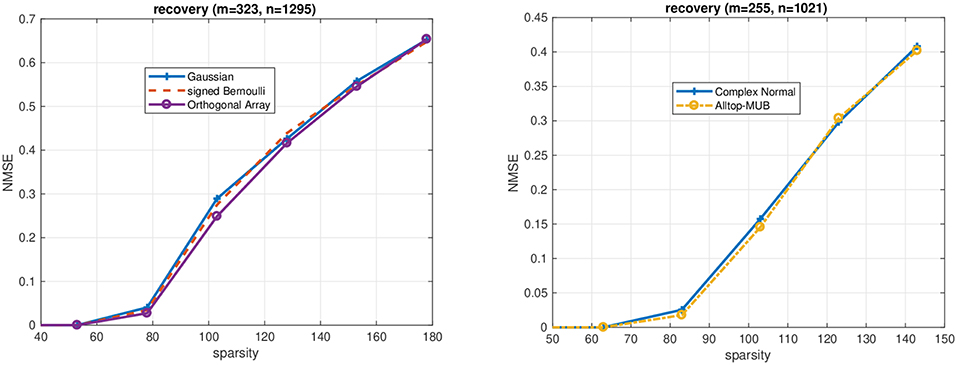
Figure 1. (Left) Performance of basis pursuit for m = 323 and n = 1295 (real-valued signals) from random orthogonal array measurements and their generic counterpart (signed Bernoulli). (Right) Performance of basis pursuit for m = 255 and n = 1021 (complex-valued signals) from random time-frequency shifted Alltop sequences and their generic counterpart (standard complex Gaussian vectors).

Numerical results for the Alltop design: Figure 1 shows the NMSE achieved for measurement matrices based on subsampling from an Alltop-design (6). The data is obtained in the same way as above, but the sparse vectors are generated as iid. complex-normal distributed on the support. For comparison the results for a (complex) standard Gaussian sampling matrix are included as well. Again, the performance of random Alltop-design measurements essentially matches its generic (Gaussian) counterpart.

5. Additional Proofs

5.1. Proof of Theorem 7

The proof is based on rather straightforward modifications of Tropp's proof for Mendelson's small ball method [37]. Let a ∈ ℂⁿ be a complex-valued random vector. Suppose that ${\text{a}}_1,\dots ,{\text{a}}_m\in {ℂ}^n$ are independent copies of a and let A be the m × n matrix whose i-th row is given by a_i. The goal is to obtain a lower bound on ${inf}_{\text{z}\in E}{\Vert \text{A}\text{z}\Vert }_{{\ell }_2},$ where E ⊂ ℂⁿ is an arbitrary set. First, note that ℓ₁ and ℓ₂ norms on ℝ^2m are related via ${\Vert \text{v}\Vert }_{{\ell }_1}\le \sqrt{2m}{\Vert \text{v}\Vert }_{{\ell }_2}$. For any z ∈ E this relation ensures

$\begin{array}{l}\Vert \text{A}\text{z}{\Vert }_{{\ell }_2}=\sqrt{{\displaystyle \sum _{i=1}^m}|\langle {\text{a}}_i,\text{z}\rangle {|}^2}=\sqrt{{\displaystyle \sum _{i=1}^m}\text{Re}{(\langle {\text{a}}_i,\text{z}\rangle )}^2+{\displaystyle \sum _{i=1}^m}\text{Im}{(\langle {\text{a}}_i,\text{z}\rangle )}^2}\\ \ge \frac{1}{\sqrt{2m}}\left({\displaystyle \sum _{i=1}^m}|\text{Re}(\langle {\text{a}}_i,\text{z}\rangle )|+{\displaystyle \sum _{i=1}^m}|\text{Im}(\langle {\text{a}}_i,\text{z}\rangle )|\right)\\ =\frac{1}{\sqrt{2m}}{\displaystyle \sum _{i=1}^m}(|\text{Re}(\langle {\text{a}}_i,\text{z}\rangle )|+|\text{Im}(\langle {\text{a}}_i,\text{z}\rangle )|).\end{array}$

Next, fix ξ > 0 and introduce the indicator function $\mathbb{\text{I}}${x ≥ ξ} which obeys x ≥ ξ$\mathbb{\text{I}}${x ≥ ξ} for all x ≥ 0. Consequently,

$\begin{array}{ll}\Vert \text{A}\text{z}{\Vert }_{{\ell }_2}\ge \frac{\xi }{\sqrt{2m}}{\displaystyle \sum _{i=1}^m}\left(\mathbb{\text{I}}\left\{|\text{Re}(\langle {\text{a}}_i,\text{z}\rangle )|\ge \xi \right\}+\mathbb{\text{I}}\left\{|\text{Im}(\langle {\text{a}}_i,\text{z}\rangle )|\ge \xi \right\}\right).& (21)\end{array}$

Also, note that the expectation value of each summand obeys

$\begin{array}{l}\mathbb{\text{E}}\left[\mathbb{\text{I}}\left\{|\text{Re}(\langle {\text{a}}_i,\text{z}\rangle )|\ge \xi \right\}\right]+\mathbb{\text{E}}\left[\mathbb{\text{I}}\left\{|\text{Im}(\langle {\text{a}}_i,\text{z}\rangle )|\ge \xi \right\}\right]\\ =\text{Pr}\left[|\text{Re}(\langle {\text{a}}_i,\text{z}\rangle )|\ge \xi \right]+\text{Pr}\left[|\text{Im}(\langle {\text{a}}_i,\text{z}\rangle )|\ge \xi \right]\\ \ge \text{Pr}\left[|\text{Re}(\langle {\text{a}}_i,\text{z}\rangle )|\ge \xi \vee |\text{Im}(\langle {\text{a}}_i,\text{z}\rangle )|\ge \xi \right]\\ \ge \text{Pr}\left[|\langle {\text{a}}_i,\text{z}\rangle |\ge \sqrt{2}\xi \right],\end{array}$

according to the union bound. The last line follows from a simple observation. Let z = a + ib be a complex number. Then, $|z|=\sqrt{a^2+b^2}\ge \sqrt{2}\xi$ necessarily implies either |a| ≥ ξ, or |b| ≥ ξ (or both). Next, define

$\begin{array}{l}{Q}_{2\xi }(\text{z})=\text{Pr}\left[|\text{Re}(\langle {\text{a}}_i,\text{z}\rangle )|\ge 2\xi \right]+\text{Pr}\left[|\text{Im}(\langle {\text{a}}_i,\text{z}\rangle )|\ge 2\xi \right]\end{array}$

and note that the estimate from above ensures

$\begin{array}{ll}{\displaystyle \underset{\text{z}\in E}{inf}}{Q}_{2\xi }(\text{z})\ge {\displaystyle \underset{\text{z}\in E}{inf}}\text{Pr}\left[|\langle \text{a},\text{z}\rangle |\ge 2^{3/2}\xi \right]=Q_{2^{3/2}\xi }(\text{a},E).& (22)\end{array}$

Adding and subtracting $\xi \sqrt{m/2}{Q}_{2\xi }(\text{z})$ to Equation (21) and taking the infimum yields

$\begin{array}{ll}\begin{array}{l}\underset{\text{z}\in E}{\inf }\Vert \mathbf{\text{Az}}{\Vert }_{{\ell }_2}\hfill \\ \ge \underset{\mathbf{\text{z}}\in E}{\inf }(\xi \sqrt{\frac{m}{2}}{Q}_{2\xi }(\mathbf{\text{z}})-\xi \sqrt{\frac{m}{2}}{Q}_{2\xi }(\mathbf{\text{z}})\hfill \\ +\frac{\xi }{\sqrt{2m}}{\displaystyle \sum _{i=1}^m\left(\mathbb{\text{I}}\left\{|\text{Re}(\langle {\mathbf{\text{a}}}_i,\mathbf{\text{z}}\rangle )|\ge \xi \right\}+\mathbb{\text{I}}\left\{|\text{Im}(\langle {\mathbf{\text{a}}}_i,\mathbf{\text{z}}\rangle )|\ge \xi \right\}\right)})\hfill \\ \ge \xi \sqrt{\frac{m}{2}}{Q}_{2^{3/2}\xi }(\mathbf{\text{a}},E)-\frac{\xi }{\sqrt{2m}}\underset{\mathbf{\text{z}}\in E}{\sup }(m{Q}_{2\xi }(\mathbf{\text{z}})\hfill \\ -{\displaystyle \sum _{i=1}^m\left(\mathbb{\text{I}}\left\{|\text{Re}(\langle {\mathbf{\text{a}}}_i,\mathbf{\text{z}}\rangle )|\ge \xi \right\}+\mathbb{\text{I}}\left\{|\text{Im}(\langle {\mathbf{\text{a}}}_i,\mathbf{\text{z}}\rangle )|\ge \xi \right\}\right)}).\hfill \end{array}& (23)\end{array}$

Here we have applied Equation (22) to bound the contribution of the first term. Since Q_2ξ(z) features both a real and imaginary part and we can split up the remaining supremum accordingly. The suprema over real and complex parts individually correspond to

$\begin{array}{l}R(E,\text{a})={\displaystyle \underset{\text{z}\in \mathbb{\text{E}}}{sup}}{\displaystyle \sum _{i=1}^m}(\text{Pr}\left[|\text{Re}(\langle {\text{a}}_i,\text{z}\rangle )|\ge 2\xi \right]-\mathbb{\text{I}}\left\{|\text{Re}(\langle {\text{a}}_i,\text{z}\rangle )|\ge \xi \right\}),\\ I(E,\text{a})={\displaystyle \underset{\text{z}\in \mathbb{\text{E}}}{sup}}{\displaystyle \sum _{i=1}^m}(\text{Pr}\left[|\text{Im}(\langle {\text{a}}_i,\text{z}\rangle )|\ge 2\xi \right]-\mathbb{\text{I}}\left\{|\text{Im}(\langle {\text{a}}_i,\text{z}\rangle )|\ge \xi \right\}),\end{array}$

and the vectors a₁, …, a_m are independent copies of a single random vector a ∈ ℂⁿ. The bounded difference inequality [45, section 6.1] asserts that both expressions concentrate around their expectation. More precisely, for any t > 0

$\begin{array}{l}\text{Pr}\left[R(E,\text{a})\ge \mathbb{\text{E}}R(E,\text{a})+t\sqrt{m}\right]\le {\text{e}}^{-t^2/2}\text{and }\\ \text{ Pr}\left[I(E,\text{a})\ge \mathbb{\text{E}}I(E,\text{a})+t\sqrt{m}\right]\le {\text{e}}^{-t^2/2}.\end{array}$

Therefore, the union bound grants a transition from R(E, a) + I(E, a) to $\mathbb{\text{E}}R(E,\text{a})+\mathbb{\text{E}}I(E,\text{a})+2\sqrt{m}t$ with probability at least 1 − 2e^−t2/2. These expectation values can be further simplified. Define the soft indicator function

${\psi }_{\xi }(s)=\{\begin{array}{ll}0\hfill & \left|s\right|\le \xi ,\hfill \\ (|s|-\xi )/\xi \hfill & \xi \le \left|s\right|\le 2\xi ,\hfill \\ 1\hfill & \left|s\right|\ge 2\xi \hfill \end{array}$

which admits the following bounds: $\mathbb{\text{I}}${|s| ≥ 2ξ} ≤ ψ_ξ(s) ≤ $\mathbb{\text{I}}${|s| ≥ ξ} for all s ∈ ℝ. Moreover, ξψ_ξ(s) is a contraction, i.e., a real-valued function with Lipschitz constant one that also obeys ξψ_ξ(0) = 0. Rademacher symmetrization [3, Lemma 8.4] and the Rademacher comparison principle [46, Equation (4.20)] yield

$\begin{array}{l}\mathbb{\text{E}}R(E,\mathbf{\text{a}})=\mathbb{\text{E}}\underset{\mathbf{\text{z}}\in E}{\sup }{\displaystyle \sum _{i=1}^m\left(\mathbb{\text{E}}\mathbb{\text{I}}\left\{|\text{Re}({\mathbf{\text{a}}}_i,\mathbf{\text{z}})|\ge 2\xi \right\}-\mathbb{\text{I}}\left\{|\text{Re}(\langle {\mathbf{\text{a}}}_i,\mathbf{\text{z}}\rangle )|\ge \xi \right\}\right)}\hfill \\ \le \mathbb{\text{E}}\underset{\mathbf{\text{z}}\in E}{\sup }{\displaystyle \sum _{i=1}^m\left(\mathbb{\text{E}}{\psi }_{\xi }(\text{Re}(\langle {\mathbf{\text{a}}}_i,\mathbf{\text{z}}\rangle ))-{\psi }_{\xi }(\text{Re}(\langle {\mathbf{\text{a}}}_i,\mathbf{\text{z}}\rangle )\right)}\hfill \\ \le 2\mathbb{\text{E}}{\displaystyle \sum _{i=1}^m{ϵ}_i}{\psi }_{\xi }(\text{Re}(\langle {\mathbf{\text{a}}}_i,\mathbf{\text{z}}\rangle )\le \frac{2}{\xi }\mathbb{\text{E}}\underset{\mathbf{\text{z}}\in E}{\sup }{\displaystyle \sum _{i=1}^m{ϵ}_i}\text{Re}(\langle {\mathbf{\text{a}}}_i,\mathbf{\text{z}}\rangle )\hfill \\ \le \frac{2\sqrt{m}}{\xi }\mathbb{\text{E}}\underset{\mathbf{\text{z}}\in E}{\sup }|\langle \mathbf{\text{z}},\mathbf{\text{h}}\rangle |,\hfill \end{array}$

where $\text{h}=\frac{1}{\sqrt{m}}\sum _{i=1}^m{ϵ}_i{\text{a}}_i\in {ℂ}^n$. A completely analogous bound holds true for $\mathbb{\text{E}}$I(E, a). Inserting both bounds into Equation (23) establishes

$\begin{array}{l}{\displaystyle \underset{\text{z}\in E}{inf}}\Vert \text{A}\text{z}{\Vert }_{{\ell }_2}\ge \xi \sqrt{\frac{m}{2}}{Q}_{2^{3/2}\xi }-\frac{\xi }{\sqrt{2m}}\left(\frac{4\sqrt{m}}{\xi }\mathbb{\text{E}}{\displaystyle \underset{\text{z}\in E}{sup}}|\langle \text{z},\text{h}\rangle |+2\sqrt{mt}\right)\\ =\xi \sqrt{\frac{m}{2}}{Q}_{2^{3/2}\xi }-2^{3/2}\mathbb{\text{E}}{\displaystyle \underset{\text{z}\in E}{sup}}|\langle \text{z},\text{h}\rangle |-\sqrt{2}\xi t\end{array}$

with probability at least 1 − 2e^−t2/2. Setting $W_m(E,\text{z})=\mathbb{\text{E}}{sup}_{\text{z}\in E}|\langle \text{z},\text{ h}\rangle |$ establishes the claim.

5.2. Proof of Lemma 2

The inclusion T_s ⊂ 2conv(Σ_s) remains valid in the complex case. Moreover, every z ∈ conv(Σ_s) necessarily obeys

$\begin{array}{l}{\displaystyle \underset{\text{z}\in \text{conv}({\Sigma }_s)}{max}}{\Vert \text{z}\Vert }_{{\ell }_1}\le {\displaystyle \underset{\text{z}\in {\Sigma }_s}{max}}{\Vert \text{z}\Vert }_{{\ell }_1}=\sqrt{s},\end{array}$

because the maximum value of a convex function is achieved at the boundary. Hoelder's inequality therefore implies

$\begin{array}{l}{W}_m(\text{a},T_s)=\mathbb{\text{E}}{\displaystyle \underset{\text{z}\in T_s}{sup}}|\langle \text{z},\text{ h}\rangle |\le 2\mathbb{\text{E}}{\displaystyle \underset{\text{z}\in \text{conv}({\Sigma }_s)}{sup}}{\Vert \text{z}\Vert }_{{\ell }_1}\Vert \text{h}{\Vert }_{{\ell }_{\infty }}\\ \le 2\sqrt{s}\mathbb{\text{E}}\Vert \text{h}{\Vert }_{{\ell }_{\infty }},& (24)\end{array}$

where $\text{h}=\frac{1}{\sqrt{m}}\sum _{i=1}^m{ϵ}_i{\text{a}}_i\in {ℂ}^n$. Moreover,

$\begin{array}{r}\mathbb{\text{E}}\Vert \mathbf{\text{h}}{\Vert }_{{\ell }_{\infty }}=\mathbb{\text{E}}\underset{1\le k\le n}{\max }|\langle {\mathbf{e}}_k,\mathbf{\text{h}}\rangle |\le \mathbb{\text{E}}\underset{1\le k\le n}{\max }|\text{Re}(\langle {\mathbf{\text{e}}}_k,\mathbf{\text{h}}\rangle )|\hfill \\ \hfill +\mathbb{\text{E}}\underset{{}_{1\le k\le n}}{\max }|\text{Im}(\langle {\mathbf{\text{e}}}_k,\mathbf{\text{h}}\rangle |\end{array}$

and we may bound both expressions on the r.h.s. independently. For the first term, fix θ > 0 and use Jensen's inequality (the logarithm is a concave function) to obtain

$\begin{array}{l}\mathbb{\text{E}}{\displaystyle \underset{1\le k\le n}{max}}|\text{Re}(\langle {\text{e}}_k,\text{h}\rangle )|=\mathbb{\text{E}}{\displaystyle \underset{1\le k\le n}{max}}{\displaystyle \underset{\sigma =\pm }{max}}\sigma \text{Re}(\langle {\text{e}}_k,\text{h}\rangle )\\ \le \frac{1}{\theta }log\left(\mathbb{\text{E}}exp\left({\displaystyle \underset{1\le k\le n}{max}}{\displaystyle \underset{\sigma =\pm }{max}}\theta \sigma \text{Re}(\langle {\text{e}}_k,\text{h}\rangle )\right)\right).\end{array}$

Monotonicity and non-negativity of the exponential function then imply

$\begin{array}{l}\mathbb{\text{E}}exp\left({\displaystyle \underset{1\le k\le n}{max}}{\displaystyle \underset{\sigma =\pm }{max}}\theta \sigma \text{Re}(\langle {\text{e}}_k,\text{h}\rangle )\right)\\ \le {\displaystyle \sum _{k=1}^n}{\displaystyle \sum _{\sigma =\pm }}\mathbb{\text{E}}exp(\theta \sigma \text{Re}(\langle {\text{e}}_k,\text{h}\rangle ))\\ ={\displaystyle \sum _{k=1}^n}{\displaystyle \sum _{\sigma =\pm }}{\displaystyle \prod _{i=1}^m}\mathbb{\text{E}}exp\left(\frac{\theta \sigma }{\sqrt{m}}{ϵ}_i\text{Re}(\langle {\text{e}}_k,{\text{a}}_i\rangle )\right),\end{array}$

where we have also used that all ϵ_i's and a_i's are independent. The remaining moment generating functions can be bounded individually. Fix 1 ≤ k ≤ n, σ ∈ {±1} and 1 ≤ i ≤ m and exploit the Rademacher randomness to infer

$\begin{array}{l}\mathbb{\text{E}}exp\left(\frac{\theta \sigma }{\sqrt{m}}{ϵ}_i\text{Re}(\langle {\text{e}}_k,{\text{a}}_i\rangle )\right)=\mathbb{\text{E}}cosh\left(\frac{\theta \sigma }{\sqrt{m}}\text{Re}(\langle {\text{e}}_k,{\text{a}}_i\rangle )\right)\\ \le \mathbb{\text{E}}exp\left(\frac{{\theta }^2{\sigma }^2}{2m}\text{Re}{(\langle {\text{e}}_k,{\text{a}}_i\rangle )}^2\right)\\ =\mathbb{\text{E}}exp\left(\frac{{\theta }^2}{2m}\text{Re}{(\langle {\text{e}}_k,{\text{a}}_i\rangle )}^2\right),\end{array}$

because σ² = 1. Incoherence moreover ensures $(\text{Re}{(\langle {\mathbf{\text{e}}}_k,{\mathbf{\text{a}}}_i\rangle )}^2\le |\langle {\mathbf{\text{e}}}_k,{\mathbf{\text{a}}}_i\rangle {|}^2\le 1$. This ensures that the remaining expectation value is upper-bounded by $exp\left(\frac{{\theta }^2}{2m}\right)$. Inserting these individual bounds into the original expression yields

$\begin{array}{l}\mathbb{\text{E}}{\displaystyle \underset{1\le k\le n}{max}}|\text{Re}(\langle {\text{e}}_k,\text{h}\rangle )|\le \frac{1}{\theta }log\left({\displaystyle \sum _{k=1}^n}{\displaystyle \sum _{\sigma =\pm }}{\displaystyle \prod _{i=1}^m}\mathbb{\text{E}}exp\left(\frac{\theta \sigma }{\sqrt{m}}{ϵ}_i\text{Re}(\langle {\text{e}}_k,{\text{a}}_i\rangle )\right)\right)\\ \le \frac{1}{\theta }log\left({\displaystyle \sum _{k=1}^n}{\displaystyle \sum _{\sigma =\pm }}{\displaystyle \prod _{i=1}^m}exp\left(\frac{{\theta }^2}{2m}\right)\right)\\ =\frac{1}{\theta }log\left(2nexp\left(\frac{{\theta }^2}{2}\right)\right)=\frac{log(2n)}{\theta }+\frac{\theta }{2}\end{array}$

for any $0<\theta \le \sqrt{2m}$. Choosing $\theta =\sqrt{2log(2n)}$ minimizes this upper bound and is feasible, by assumption. A completely analogous bound can be derived for the expected maximum absolute value of the imaginary part. Combining both yields

$\begin{array}{l}\mathbb{\text{E}}\Vert \text{h}{\Vert }_{{\ell }_{\infty }}\le \sqrt{2log(2n)}+\sqrt{2log(2n)}=2\sqrt{2log(2n)}\end{array}$

and inserting this bound into (24) ensures

$\begin{array}{l}{W}_m(\text{a},T_s)\le 4\sqrt{2slog(2n)}.\end{array}$

Author Contributions

RK developed the technical aspects of the paper. PJ is responsible for the numerical aspects and the discussion of orthogonal arrays. Some of the main conceptual ideas are due to DM. These in particular include the idea of employing orthogonal arrays to partially derandomize signed Bernoulli matrices and the insight that a partial de-randomization of Gordon's escape through a mesh is essential for achieving the results. All authors contributed to the introduction and general presentation.

Funding

PJ is supported by the DFG grant JU 2795/3 and DAAD grant 57417688. RK was in part supported by Joel A. Tropp under the ONR Award No. N00014-17-12146 and also acknowledges funding provided by the Institute of Quantum Information and Matter, an NSF Physics Frontiers Center (NSF Grant PHY-1733907). DM was partially supported by AFOSR FA9550-18-1-0107, NSF DMS 1829955, and the Simons Institute of the Theory of Computing. We acknowledge support by the German Research Foundation and the Open Access Publication Fund of TU Berlin.

Conflict of Interest Statement

The authors declare that the research was conducted in the absence of any commercial or financial relationships that could be construed as a potential conflict of interest.

Acknowledgments

The authors want to thank David Gross for providing the original ideas that ultimately led to this publication.

Footnotes

1. ^Existing deterministic constructions (see e.g., Bandeira et al.[13]), do not (yet) yield comparable statements.

2. ^For comparison, a complex standard Gaussian vector obeys $\mathbb{\text{E}}\left[|\langle \text{z},{\text{a}}_g\rangle {|}^{2k}\right]=k!{\Vert \text{z}\Vert }_{{\ell }_2}^{2k}$ instead.

3. ^This is a m × n matrix where each entry is sampled independently from the standard normal distribution ${N}(0,1)$.

4. ^For example http://neilsloane.com/oadir/ or http://pietereendebak.nl/oapage/

References

1. Donoho DL. Compressed sensing. IEEE Trans Inform Theory. (2006) 52:1289–306. doi: 10.1109/TIT.2006.871582

CrossRef Full Text | Google Scholar

2. Candes EJ, Romberg J, Tao T. Robust uncertainty principles: exact signal reconstruction from highly incomplete frequency information. IEEE Trans Inform Theory. (2006) 52:489–509. doi: 10.1109/TIT.2005.862083

CrossRef Full Text | Google Scholar

3. Foucart S, Rauhut H. A Mathematical Introduction to Compressive Sensing. Applied and Numerical Harmonic Analysis. New York, NY: Birkhäuser/Springer (2013). doi: 10.1007/978-0-8176-4948-7

CrossRef Full Text | Google Scholar

4. Eldar YC, Kutyniok G. Compressed Sensing: Theory and Applications. Cambridge, UK: Cambridge University Press (2012).

Google Scholar

5. Candès EJ, Strohmer T, Voroninski V. Phaselift: exact and stable signal recovery from magnitude measurements via convex programming. Commun Pure Appl Math. (2013) 66:1241–74. doi: 10.1002/cpa.21432

CrossRef Full Text | Google Scholar

6. Candès E, Li X. Solving quadratic equations via PhaseLift when there are about as many equations as unknowns. Found Comput Math. (2013). p. 1–10. doi: 10.1007/s10208-013-9162-z

CrossRef Full Text | Google Scholar

7. Gross D, Krahmer F, Kueng R. A partial derandomization of phaseLift using spherical designs. J Fourier Anal Appl. (2015) 21:229–66. doi: 10.1007/s00041-014-9361-2

CrossRef Full Text | Google Scholar

8. Kueng R, Rauhut H, Terstiege U. Low rank matrix recovery from rank one measurements. Appl Comput Harmon Anal. (2017) 42:88–116. doi: 10.1016/j.acha.2015.07.007

CrossRef Full Text | Google Scholar

9. Kabanava M, Kueng R, Rauhut H, Terstiege U. Stable low-rank matrix recovery via null space properties. Inform Inference. (2016) 5:405–41. doi: 10.1093/imaiai/iaw014

CrossRef Full Text | Google Scholar

10. Kueng R, Gross D, Krahmer F. Spherical designs as a tool for derandomization: the case of PhaseLift. In: 2015 International Conference on Sampling Theory and Applications (Washington, DC: SampTA) (2015). p. 192–6. doi: 10.1109/SAMPTA.2015.7148878

CrossRef Full Text | Google Scholar

11. Kueng R, Zhu H, Gross D. Low rank matrix recovery from Clifford orbits. arXiv [Preprint] (2016). arXiv:161008070.

Google Scholar

12. Tropp JA. A mathematical introduction to compressive sensing [Book Review]. Bull Amer Math Soc. (2017) 54:151–65. doi: 10.1090/bull/1546

CrossRef Full Text | Google Scholar

13. Bandeira AS, Fickus M, Mixon DG, Wong P. The road to deterministic matrices with the restricted isometry property. J Fourier Anal Appl. (2013) 19:1123–49. doi: 10.1007/s00041-013-9293-2

CrossRef Full Text | Google Scholar

14. Rudelson M, Vershynin R. On sparse reconstruction from Fourier and Gaussian measurements. Commun Pure Appl Math. (2008) 61:1025–45. doi: 10.1002/cpa.20227

CrossRef Full Text | Google Scholar

15. Cheraghchi M, Guruswami V, Velingker A. Restricted isometry of fourier matrices and list decodability of random linear codes. SIAM J Comput. (2013) 42:1888–914. doi: 10.1137/120896773

CrossRef Full Text | Google Scholar

16. Hedayat AS, Sloane NJA, Stufken J. Orthogonal Arrays: Theory and Applications New York, NY: Springer-Verlag (1999). doi: 10.1007/978-1-4612-1478-6

CrossRef Full Text | Google Scholar

17. Delsarte P, Goethals JM, Seidel JJ. Spherical codes and designs. Geometriae Dedicata. (1997) 6:363–88. doi: 10.1007/BF03187604

CrossRef Full Text | Google Scholar

18. Bajnok B. Construction of spherical t-designs. Geom Dedicata. (1992) 43:167–79. doi: 10.1007/BF00147866

CrossRef Full Text | Google Scholar

19. Korevaar J, Meyers JLH. Chebyshev-type quadrature on multidimensional domains. J Approx Theory. (1994) 79:144–64. doi: 10.1006/jath.1994.1119

CrossRef Full Text | Google Scholar

20. Hayashi A, Hashimoto T, Horibe M. Reexamination of optimal quantum state estimation of pure states. Phys Rev A. (2005) 72:032325. doi: 10.1103/PhysRevA.72.032325

CrossRef Full Text | Google Scholar

21. Bandyopadhyay S, Boykin PO, Roychowdhury V, Vatan F. A new proof for the existence of mutually unbiased bases. Algorithmica. (2002) 34:512–8. doi: 10.1007/s00453-002-0980-7

CrossRef Full Text | Google Scholar

22. Klappenecker A, Rotteler M. Mutually unbiased bases are complex projective 2-designs. In: A. Klappenecker, M. Roetteler Editors. Proceedings International Symposium on Information Theory, 2005. (Adelaide, AU: ISIT) (2005). p. 1740–4. doi: 10.1109/ISIT.2005.1523643

CrossRef Full Text | Google Scholar

23. Klappenecker A, Rötteler M. Constructions of Mutually Unbiased Bases. In: Mullen GL, Poli A, Stichtenoth H, editors. Finite Fields and Applications. Berlin; Heidelberg: Springer (2004). p. 137–44. doi: 10.1007/978-3-540-24633-6-10

CrossRef Full Text | Google Scholar

24. Alltop W. Complex sequences with low periodic correlations. IEEE Trans Inform Theory. (1980) 26:350–4. doi: 10.1109/TIT.1980.1056185

CrossRef Full Text | Google Scholar

25. Bourgain J, Dilworth S, Ford K, Konyagin S, Kutzarova D. Explicit constructions of RIP matrices and related problems. Duke Math J. (2011) 159:145–85. doi: 10.1215/00127094-1384809

CrossRef Full Text | Google Scholar

26. Mixon DG. In: Boche H, Calderbank R, Kutyniok G, Vybíral J, editors. Explicit Matrices With the Restricted Isometry Property: Breaking the Square-Root Bottleneck. Cham: Springer International Publishing (2015). p. 389–417. doi: 10.1007/978-3-319-16042-9-13

CrossRef Full Text | Google Scholar

27. Bandeira AS, Mixon DG, Moreira J. A conditional construction of restricted isometries. Int Math Res Notices. (2017) 2017:372–81. doi: 10.1093/imrn/rnv385

CrossRef Full Text | Google Scholar

28. Bandeira AS, Fickus M, Mixon DG, Moreira J. Derandomizing restricted isometries via the legendre symbol. Constr Approx. (2016) 43:409–24. doi: 10.1007/s00365-015-9310-6

CrossRef Full Text | Google Scholar

29. Baraniuk R, Davenport M, DeVore R, Wakin M. A simple proof of the restricted isometry property for random matrices. Constr Approx. (2008) 28:253–63. doi: 10.1007/s00365-007-9003-x

CrossRef Full Text | Google Scholar

30. Krahmer F, Ward R. New and improved johnson-Lindenstrauss embeddings via the restricted isometry property. SIAM J Math Anal. (2011) 43:1269–81. doi: 10.1137/100810447

CrossRef Full Text | Google Scholar

31. Kane DM, Nelson J. A derandomized sparse Johnson-Lindenstrauss transform. arXiv [Preprint] (2010). arXiv:10063585.

Google Scholar

32. Duarte MF, Davenport MA, Takhar D, Laska JN, Sun T, Kelly KF, et al. Single-pixel imaging via compressive sampling. IEEE Signal Process Magaz. (2008) 25:83–91. doi: 10.1109/MSP.2007.914730

CrossRef Full Text | Google Scholar

33. Herman MA, Strohmer T. High-resolution radar via compressed sensing. IEEE Trans Signal Process. (2009) 57:2275–84. doi: 10.1109/TSP.2009.2014277

CrossRef Full Text | Google Scholar

34. Tropp JA, Dhillon IS, Heath RW, Strohmer T. CDMA signature sequences with low peak-to-average-power ratio via alternating projection. In: The Thrity-Seventh Asilomar Conference on Signals, Systems Computers. Pacific Grove, CA (2003). p. 475–9.

Google Scholar

35. Kabanava M, Rauhut H. Analysis ℓ₁-recovery with frames and gaussian measurements. Acta Appl Math. (2015) 140:173–95. doi: 10.1007/s10440-014-9984-y

CrossRef Full Text | Google Scholar

36. Dirksen S, Lecue G, Rauhut H. On the gap between restricted isometry properties and sparse recovery conditions. IEEE Trans Inform Theory. (2016) 99:1.

Google Scholar

37. Tropp JA. Convex Recovery of a Structured Signal from Independent Random Linear Measurements. In: Pfander EG, editor. Sampling Theory, a Renaissance: Compressive Sensing and Other Developments. Birkhäuser: Springer International Publishing (2015). p. 67–101. doi: 10.1007/978-3-319-19749-4-2

CrossRef Full Text | Google Scholar

38. Gordon Y. On Milman's inequality and random subspaces which escape through a mesh in ℝⁿ. In: Lindenstrauss J, Milman VD, editors. Geometric Aspects of Functional Analysis. Berlin; Heidelberg: Springer Berlin Heidelberg (1988). p. 84–106. doi: 10.1007/BFb0081737

CrossRef Full Text

39. Dudley R. Sizes of compact subsets of Hilbert space and continuity of Gaussian processes. J Funct Anal. (1967) 1:290–330. doi: 10.1016/0022-1236(67)90017-1

CrossRef Full Text | Google Scholar

40. Mendelson S. Learning without concentration. J ACM. (2015) 62:21:25. doi: 10.1145/2699439

CrossRef Full Text | Google Scholar

41. Koltchinskii V, Mendelson S. Bounding the smallest singular value of a random matrix without concentration. Int Math Res Notices. (2015) 2015:12991–3008. doi: 10.1093/imrn/rnv096

CrossRef Full Text | Google Scholar

42. Rao CR. Factorial experiments derivable from combinatorial arrangements of arrays. J R Stat Soc. (1947) 9:128–39. doi: 10.2307/2983576

CrossRef Full Text | Google Scholar

43. Pat A. On Construction of a Class of Orthogonal Arrays. Ph.D. Thesis, Department of Mathematics, Indian Institute of Technology, Kharagpur, India. (2012).

Google Scholar

44. Kueng R, Jung P. Robust nonnegative sparse recovery and the nullspace property of 0/1 measurements. IEEE Trans Inform Theory. (2018) 64:689–703. doi: 10.1109/TIT.2017.2746620

CrossRef Full Text | Google Scholar

45. Boucheron S, Lugosi G, Massart P. Concentration Inequalities: A Nonasymptotic Theory of Independence. Oxford: Oxford University Press (2013). doi: 10.1093/acprof:oso/9780199535255.001.0001

CrossRef Full Text | Google Scholar

46. Ledoux M, Talagrand M. Probability in Banach Spaces: Isoperimetry and Processes. Berlin; Heidelberg: Springer Science & Business Media (2013).

Google Scholar