Chimera States With 2D Deterministic and Random Fractal Connectivity

1. Introduction

A Chimera state is characterized by the unexpected coexistence of coherent and incoherent domains in networks of coupled oscillators. Chimera states were first discovered in 2002 in a system of coupled Kuramoto phase oscillators [1, 2] and were further established 2 years later in a seminal work by Abrams and Strogatz [3]. They captivated scientific interest during the past 15 years due to their intriguing structural and dynamical properties and to potential applications in physics [4–7], chemistry [8–10], and biology [11–16]. Although original studies referred to coupled phase oscillators, later works have reported chimera states in coupled FitzHugh-Nagumo, Hindmarsh-Rose, Van der Pol, and Leaky Integrate-and-Fire (LIF) oscillator networks [17–24]. Most recent advances in the general domain of local synchronization are summarized in review articles [25–29].

Previous studies on 2D nonlocal connectivity with periodic, toroidal boundary conditions have demonstrated a variety of chimera patterns. Using the phase oscillator, the FitzHugh Nagumo system or the LIF neuron oscillators chimera patterns emerged in the form of coherent and incoherent single or multiple spots, rings, lines, and grids of spots [19, 30–34]. Some of these patterns, come as generalizations of the 1D chimera forms to 2D geometry (e.g., spots and stripes), while others are new patterns which do not have an analogy in 1D (e.g., spiral waves).

As early structural studies of the human brain, using Magnetic Resonance Imaging (MRI) techniques and Diffusion Tensor Imaging (DTI) analysis, have captured fractal attributes and self-similarities in the structure of the neuron axons network [35–39], recent numerical studies have introduced fractal, hierarchical connectivity in the simulations of networks of spiking neurons. The use of Cantor-type connectivities in 1D ring networks has demonstrated that the induced chimera states retain some of the fractal features of the Cantor connectivity schemes [18, 21, 40–44]. More recently 2D simulations of chimera states were attempted, using the LIF model with symmetric Sierpinski-carpet connectivity and first evidence was provided that for small values of the coupling strength single asynchronous spots are formed which acquire hierarchical structure, reminiscent of the Sierpinski connectivity matrix [45]. This was a first study, providing evidence of hierarchical chimeras in 2D networks.

In the present study we confirm the presence of hierarchical chimeras for different parameter values (especially for different refractory periods) in 2D LIF networks and we extend our study to slanted fractals and random fractal connectivity schemes. We provide evidence of asymmetric hierarchical chimera states, multiple incoherent spot chimeras with internal hierarchical connectivity which fades away with time, as well as stable patterns where coherent spots, incoherent domains, and traveling waves coexist.

We would like to stress here, that the aim of this study is not to simulate in detail the three-dimensional connectivity of the human brain, based on the MRI recordings. Rather, this research is inspired by the fractal and multifractal analysis of the MRI images, which indicate that the neuron axons are not homogeneously distributed in the brain but they span a subspace with fractal dimension d_f ≈ 2.5. These fractal attributes have been computed for length scales between [1 and 10 cm] using the box-counting technique [36–38]. The present study aims to address the influence of fractal connectivity (as opposed to the usual non-local connectivity) in the formation of chimera states. Although chimera states with hierarchical connectivity in one-dimensions have been studied in many works [18, 21, 41, 42, 44], the problem of hierarchical connectivity in two-dimensions has not been adequately addressed. To this end, several drastic simplifications were made due mostly to limitations of computational resources: (a) the LIF model is used which is a minimal model addressing the biological neuron activity, (b) only restricted system sizes are considered as will be described in the next section, (c) the connectivity was reduced to a flat fractal kernel, and (d) periodic boundary conditions are considered in order to retain the symmetry of interactions. All these simplifications aim to avoid including too many parameters in the system and to focus on the mechanisms producing hierarchical chimera patterns and 2D spiral wave chimeras.

In the next section we give a brief presentation of the LIF model and its implementation on a 2D network with deterministic and random fractal connectivity. In section 3.1 we present our results when the fractal connectivity is deterministic and symmetric, while the slanted fractal case is presented in section 3.2. Our results on random fractal connectivity are presented in section 4 where we report the finding of spiral wave chimeras and chimeras exhibiting three different coexisting domain types: coherent, incoherent and traveling waves. The conclusions of this study are briefly summarized in the final section 5 and relevant open issues are discussed.

2. The Model and the Connectivity Schemes

The LIF model for single neuron dynamics was introduced by Louis Lapicque in 1907 and is in frequent use by computational neuroscientists due to its easy numerical implementation, while it retains the main dynamical features of biological neuron activity [46–48]. In relation to collective neuron dynamics, coupled LIF neurons were shown to produce chimera states under various types of non-local connectivity schemes in 1D [22–24, 41, 49–51], in 2D [19, 45], and in 3D [52].

In this section, we present the LIF coupling scheme in 2D using different fractal connectivity geometries. Namely, after recapitulating the LIF dynamics in 2D for a generic coupling matrix, we introduce the following coupling schemes: (a) symmetric deterministic Sierpinski carpet, (b) slanted deterministic Sierpinski carpet, and (c) random Sierpinski carpet (which is almost always asymmetric). These coupling schemes will be used in sections 3 and 4 for studying local synchronization phenomena.

2.1. The LIF Coupling Scheme

The dynamics describing the temporal evolution of the potential u_ij(t) of a neuron having Cartesian coordinates (i, j) is divided in three phases: (i) the integration phase shown below in Equation (1a) characterized by a linear differential equation exhibiting an exponential increase of the membrane potential, (ii) the abrupt resetting phase (Equation 1b) and (iii) a refractory period (Equation 1c). These phases are expressed by the following equations:

$\begin{array}{ll}\frac{d{u}_{ij}(t)}{dt}=\mu -u_{ij}(t)-\frac{1}{N_c}{\displaystyle \sum _{kl\in \{N_{ij}\}}^{}}{\sigma }_{ijkl}\left[u_{kl}(t)-u_{ij}(t)\right]& (\mathrm{1a})\end{array}$

$\begin{array}{ll}{\displaystyle \underset{ϵ\to 0}{lim}}{u}_{ij}(t_r+ϵ)\to u_{\text{rest}},\text{ when }{u}_{ij}(t_r)\ge u_{\text{th}},r=1,2,\cdots & (\mathrm{1b})\end{array}$

$\begin{array}{ll}{u}_{ij}(t)=u_{\text{rest}},\text{ when }{t}_r\le t<t_r+T_r,& (\mathrm{1c})\end{array}$

On the right hand side of Equation (1a), the first two terms correspond to the integration of the potential while the last term accounts for the exchange between neuron (i, j) and other neurons in the network.

The various parameters in Equation (1) have the following interpretation: The variable u_th defines the maximum value that the potentials u_ij can take, after which the oscillators are reset to their rest potential u_rest. The resetting times t_r are counted by the index r = 1, 2, ⋯ . μ is the value that the potential of the neuron (i, j) would asymptotically tend to if there was no resetting condition, u_th < μ. T_r is a refractory period after resetting, during which the neuron potential remains at the rest state. N_c is the number of neurons that are connected with the neuron (i, j). These neurons are members of the set {N_ij}.

In the present study we assume that all oscillators are identical, they have identical parameters: μ, u_rest, u_th and N_c. For simplicity, we also assume that the coupling is linear and every oscillator is linked to all others through a coupling matrix, whose element σ_ijkl links oscillators (i, j) and (k, l). The values of the matrix elements may take any value (positive, negative, or zero), depending on the connectivity of the network, but in the current study we restrict the coupling matrix elements to the interval 0 ≤ σ_ijkl ≤ 0.3 .

The solution of Equation (1) in the absence of coupling provides the period T_s of the single neuron and the corresponding phase velocity ω_s (the subscript “s” stands for “single”, uncoupled neuron), as:

$\begin{array}{ll}{T}_s=ln\frac{\mu -u_{\text{rest}}}{\mu -u_{\text{th}}}+T_r,{\omega }_s=2\pi /T_s.& (2)\end{array}$

Although all neurons have the same parameters when uncoupled, coupling induces local and global variations in the period of the individual neurons and the network acquires a distribution of mean phase velocities. This distribution characterizes the collective behavior of the network. The mean phase velocity of all coupled neurons ω_ij in a time interval Δt is computed as:

$\begin{array}{ll}{\omega }_{ij}=\frac{2\pi Z_{ij}(\Delta t)}{\Delta t}& (3)\end{array}$

where Z_ij(Δt) is the integer number of full cycles that neuron (i, j) has completed in the time interval Δt, and is computed numerically during the simulations. The relative values of ω are of central importance when studying chimera states, because they differentiate between the coherent and incoherent domains. In the coherent domains all the elements have common mean phase velocities, while the incoherent domains are characterized by a distribution of ω-values [17].

2.2. Connectivity Schemes

In the present study the neuron oscillators are arranged on a 2D lattice-network of size N × N. The three fractals used to construct the connections of the LIF oscillators are Sierpinski carpets, which are flat fractals with Hausdorff dimension ln 8/ln 3 ≈ 1.8928. The construction of the Sierpinski carpets is recursive and follows three simple algorithms:

• The deterministic symmetric Sierpinski carpet: (a) We begin with a square which we subsequently divide into 9 equal smaller squares. (b) We then remove the central square and this concludes the first iteration of the process. (c) We divide each of the remaining 8 squares into 9 equal smaller squares and remove the central one of each group of 9. (d) This concludes the second iteration. (e) The same sequence of dividing and removing can be applied arbitrarily many times to obtain as many spatial scales as required [53, 54]. The connectivity scheme which is produced is shown in Figure 1A.

• The deterministic slanted Sierpinski carpet: (a) We begin with a square which we subsequently divide into 9 equal smaller squares. (b) We then remove one of the 8 non-central squares and this concludes the first iteration of the process. In Figure 1B we have chosen to remove the lower right square. (c) We divide each of the remaining 8 squares into 9 equal smaller squares and remove the same one as in the previous iteration (lower right squares) in each group of 9. (d) This concludes the second iteration. e) The same sequence of dividing and removing can be applied arbitrarily many times to obtain the connectivity scheme depicted in Figure 1B.

• The random Sierpinski carpet: (a) We begin with a square which we subsequently divide into 9 equal smaller squares. (b) We then remove randomly one of the 9 squares and this concludes the first iteration of the process. In Figure 1C we have chosen to remove the central square. (c) We divide each of the remaining 8 squares into 9 equal smaller squares and remove one square at random from each group of 9. (d) This concludes the second iteration. (e) The same sequence of dividing and removing randomly can be applied arbitrarily many times to obtain the connectivity of Figure 1C.

FIGURE 1

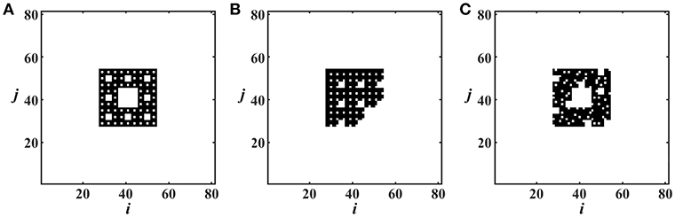
Figure 1. The Sierpinski carpets used as coupling matrices: (A) deterministic symmetric Sierpinski connectivity pattern, (B) deterministic slanted Sierpinski connectivity pattern and (C) random Sierpinski connectivity pattern. In all cases three orders of iteration are used, based on a 3 × 3 initiation square.

The resulting deterministic and random hierarchical pictures are used as connection matrices. Namely, the central node (i, j) of the connectivity scheme is only linked with all black nodes that belong to the Sierpinski carpet surrounding it. The coupling of other nodes is formed by translation of the fractals. To maintain an identical coupling scheme for all nodes we use periodic boundary conditions in both x− and y−directions, leading to a torus geometry [45].

In all three cases, symmetric deterministic, slanted deterministic or random hierarchical connectivity, if we denote by {N_ij} the set of all nonzero cells of the Sierpinski carpet centered around the node (i, j) and denote by (k, l) any arbitrary element of the system, then the coupling matrix elements σ_ijkl between nodes (i, j) and (k, l) take the form:

$\begin{array}{ll}{\sigma }_{ijkl}=\{\begin{array}{l}\sigma ,\forall (k,l)\in \left\{N_{ij}\right\}\\ 0,\text{ elsewhere}\end{array}& (4)\end{array}$

In this study the coupling strength value σ is a positive constant, common for all network connections [45]. As working parameter set we use μ = 1, u_th = 0.98, u_rest = 0 and N = 81, while N = 243 in some simulations. All simulations start with random initial conditions. For the system integration the explicit Euler scheme was used with integration step dt = 10⁻³. 4-th order Runge-Kutta was also used as a test and the results were compatible with the Euler scheme. The connectivity pattern was used directly within the Euler scheme and the iteration time was 10⁴ time units for all reported simulations. The spatial coupling was performed via direct convolution. Using an MPI parallel implementation of the algorithm on multiple (usually 20–80) CPUs each simulation took on average 8 CPU hours for 10⁴ time units. The algorithms are available online¹.

In Table 1, we present collectively all the qualitative results we obtained by scanning the parameters, 0.1 ≤ σ ≤ 0.3 and 0 ≤ T_r ≤ 2.0 (in time units). For the 2D LIF scheme (Equation 1), it is relatively easy to find chimera states in the parameter regions reported in Table 1. In these regions there is little sensitivity to initial conditions and most initial states end-up in the corresponding chimeras. Only for intermediate parameter values, between domains which support distinct chimera patterns, the different initial conditions may result to different synchronization motifs. Overall, for small σ values we observe spot chimeras many of which present structure reminiscent of the features of the connectivity matrix (see more in section 3). For larger values of σ and T_r more intricate patterns arise such as multiple spots, grids, stripes, spirals and even stable triple combinations of coherent spots, incoherent domains and traveling waves. Details on the particular patterns are given in sections 3, 4 and the Table 1.

TABLE 1

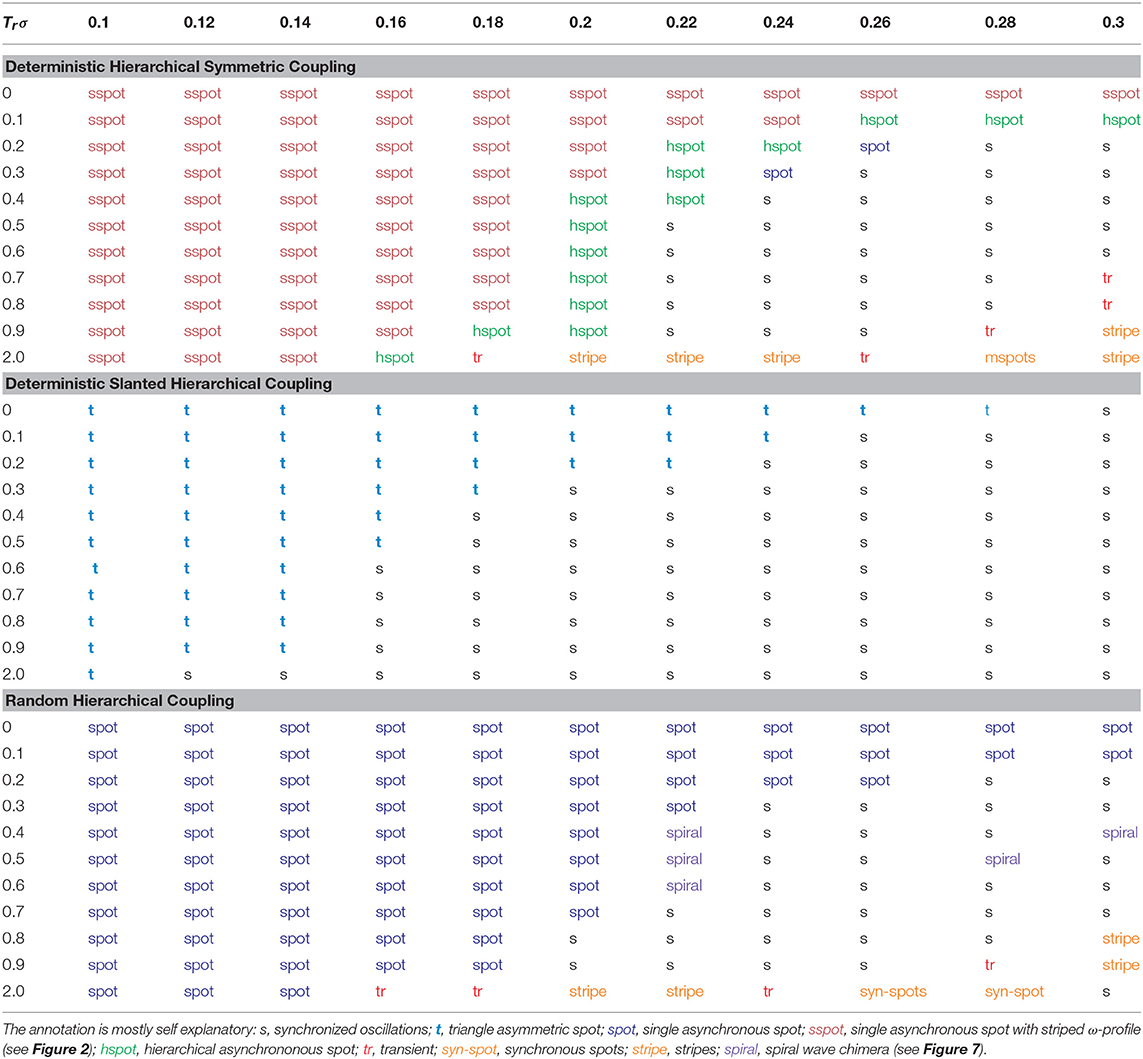
Table 1. Collective presentation of the chimera patterns in the LIF model for σ ranging between (0.1–0.3) and T_r in the interval from 0 to 2.0 time units.

3. Deterministic Fractal Connectivity

3.1. Symmetric Coupling

In a previous study, the present authors and T. Kasimatis have used the symmetric coupling of Figure 1A to explore the influence of the hierarchical connectivity in the form of 2D chimera patterns [45]. For small positive values of the coupling strength and medium values of the refractory period, T_r = 0.5 time units, they report spot chimera patterns with internal structure reminiscent of the connectivity matrix. The chimeras are best visualized in the ω-profiles, when the spots are immobile. For larger values of the coupling strength σ, stripe and grid chimeras were reported which were mostly traveling and, as a result, the hierarchical structure of the chimeras, visible in the ω-profiles, was masked. In such cases one can always resort to using the comoving frame to avoid that the motion of the spot smooths out the ω-structure, but this is outside the scope of the present study.

In the following we present evidence that hierarchical spot chimeras are possible even for T_r = 0. In Figure 2A we present the u_ij-profile for σ = 0.18 and T_r = 0. The internal structure of an asynchronous spot chimera is visible but the hierarchical scheme in Figure 2B is not as clear as it was in Argyropoulos et al. [45], where T_r = 0.5 time units was used. In this realization the incoherent elements are ordered in stripes parallel to the i-direction. Depending on the initial conditions the stripes appear parallel to the i− or to the j−direction, reflecting the square geometry of the connectivity kernel. The grid-formations in Argyropoulos et al. [45] (Figures 2B, 3B, therein) can be viewed as coexistence/superpositions of stripes in both directions.

FIGURE 2

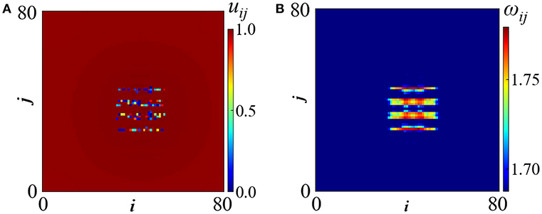
Figure 2. (A) The potential profile and (B) the mean phase velocity profile for an asynchronous spot chimera realized for symmetric hierarchical coupling with σ = 0.18 and T_r = 0. Other parameters are μ = 1, u_th = 0.98, u_rest = 0 and N = 81. The simulations start from random initial conditions.

FIGURE 3

Figure 3. The time evolution of ω for (A) element (i, j) = (0, 8) belonging to the coherent domain and (B) element (i, j) = (46, 39) belonging to the incoherent domain of Figure 2. σ = 0.18 and T_r = 0. Parameters are as in Figure 2A.

In Figure 3 we present the evolution of ω of two elements, one belonging to the coherent domain (Figure 3A), and one to the incoherent (Figure 3B). The calculations of ω were performed in time windows of Δt = 30 time units. While in the coherent domains the ω values stabilize mostly around 1.68 (with infrequent excursions to higher values), in the incoherent domains the mean phase velocity alternates between the values ω = 1.88 and ω = 1.68. This apparent bistability may reflect the slight erratic motion of the incoherent domains. Their elements may spent some time participating in the coherent domain and other time in the incoherent and thus bistability is observed in their mean phase velocity.

By increasing the system size it is possible to increase the number of incoherent domains that the system can accommodate (see Figure 4). They take the form of spiral wave multichimeras. In the present case, each of the four incoherent domains is the core region of a distinct spiral wave chimera. Around each core there is a rotating phase wave with a large wavelength. Apart from the number of asynchronous cores, larger systems (e.g., 243 × 243 in the present case) can accommodate incoherent cores with non-homogeneous internal structure, caused (as we believe) by the hierarchical ordering of the connectivity matrix. This is evident mainly in Figures 4A,B while in Figures 4C,D this internal structure is gradually destroyed due to the tiny erratic motion of the incoherent domains, giving rise to incoherent cores composed of random phases. The filamented structure of the incoherent domains in Figure 4A has been also found in 2D coupled phase oscillators [55]. In both cases the filaments are observed in the 4-chimera states and for specific parameter values. In the LIF case with fractal connectivity, these filaments are short-lived and they dissociate passing via a hierarchical phase (see Figures 4B,C) into becoming the stable incoherent domains (see Figure 4D) of the spiral chimera.

FIGURE 4

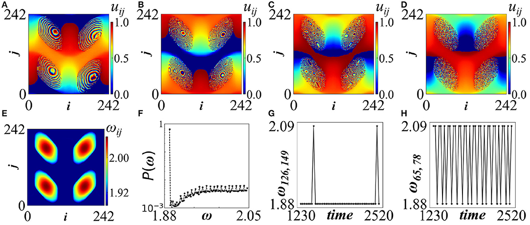
Figure 4. Top row: Spiral wave multichimera state with four incoherent cores in symmetric deterministic connectivity for system size 243 × 243; the potential profiles are depicted at times: (A) t = 1200, (B) t = 1800 (C) t = 2700 and (D) t = 10020 time units. Bottom row: (E) Mean phase velocity profile, (F) Typical histogram of mean phase velocities, (G) Time evolution of ω on a node contained in the coherent regions and (H) Time evolution of ω on a node belonging to one of the incoherent cores. Parameters are σ = 0.25 and T_r = 0.5 and N = 243. All other parameters are as in Figure 2A. Simulations start from random initial conditions. A related video is included in the Supplementary Material.

In the 2nd row of Figure 4, first the long time ω-profile is presented (Figure 4E). As the mean phase velocities change during the transition time, we record here the ω-profile after the four cores have stabilized to their full incoherent state. The ω-histogram in logarithmic scale (Figure 4F) demonstrates one very distinct peak at low frequencies which corresponds to the coherent region and one distributed region in higher frequencies, which correspond to the four incoherent spots, collectively. There is no distinctive maximum related to the incoherent cores due to the distributed ω− values in these regions. In Figures 4G,H the temporal evolution of the ω-values in the coherent and the incoherent domains are monitored during the transition period. The incoherent elements are frequently passing from low to high frequencies and thus have higher average ω as compared with the coherent ones, which mostly oscillate with low frequency. The development of this pattern is presented in a short 30s video included in the Supplementary Material².

3.2. Slanted Fractal Coupling

In the case of slanted deterministic coupling, with connectivity depicted in Figure 1B, chimera patterns are produced which are mostly traveling in the direction of the reflection symmetry axis of the kernel [56]. Because traveling is mostly accompanied by erratic motion, it is difficult to detect the fractality in the ω-profile. Figure 5 is a rare example of an immobile incoherent spot where a meaningful ω-profile can be calculated. In Figure 5A the u_ij-profile shows that the form of the chimera is not circular but takes the arrow-like shape of the seeding connectivity, Figure 1B. Besides u, also the ω−profile reflects the form of the connectivity matrix, Figure 5B.

FIGURE 5

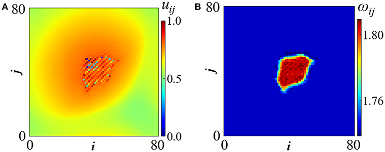
Figure 5. Chimera state with slanted fractal deterministic connectivity: (A) u_ij-profile and (B) ω_ij-profile. Parameters are σ = 0.2 and T_r = 0.1. All other parameters are as in Figure 2A. Simulations start from random initial conditions.

The external shape of the asymmetric spot, which mimics the perimeter of the oblique connectivity kernel, supports previous results in hierarchical 2D chimeras indicating that, for appropriate choices of (small) coupling strengths, the form of the kernel is mirrored in the ω-profile [45]. Here, the erratic motion of the pattern does not allow the observation of potential hierarchical internal structure in the ω−profile, induced as a result of fractal connectivity schemes as in Argyropoulos et al. [45]. A resolution of this issue involves the use of a comoving frame, but this is outside the scope of the present study.

4. Random Fractal Connectivity

Random connectivity is almost always asymmetric and this is the case we consider here. As a general observation the asymmetry of the connectivity pattern often causes motion of the chimera patterns. As an example, for σ = 0.2 and T_r = 0.5 an erratically traveling incoherent spot is formed, depicted in Figure 6. The incoherent spot potential profile, u_ij, seems to present some internal structure in the form of irregular vertical stripes (see Figure 6A). To make an analogy, we remind of the more regular, stripped structure that was reported in Figure 2 for deterministic symmetric coupling. Here, the kernel is non-symmetric and this fact together with the motion of the incoherent part makes it difficult to discern any fine details in its ω−profile (see Figure 6B). In Figure 6B the ω-profile has been calculated in time windows of size Δt = 30 time units, where the incoherent spot can be considered as almost immobile. As in all cases of traveling patterns, the use of a comoving frame could resolve possible patterns inside the incoherent part of the mean phase velocity profile. Different realizations of the fractal coupling matrix do not affect the number and sizes of the coherent and incoherent domains of the chimera pattern, provided that the fractal dimension and the hierarchical order are retained in the different realizations.

FIGURE 6

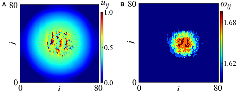
Figure 6. Single mobile spot in random fractal connectivity. Parameters are σ = 0.2 and T_r = 0.5. All other parameters are as in Figure 2A. Simulations start from random initial conditions.

Increasing slightly the coupling strengths while keeping T_r to low values, the patterns become unstable. A typical example is shown in Figure 7, where wave domains are shown spiraling around the torus. The four spiraling regions have the form of successive wavefronts with arrow-like shapes [55]. They rotate around coherent cores which are characterized by different wavelengths than the spiraling fronts. This is a new type of spiral chimera composed by coherent waves with two different wave lengths. Even in this case, we observe that the sizes of the spiraling fronts are similar to the size of the initiation connectivity pattern. A related video is added in the Supplementary Material².

FIGURE 7

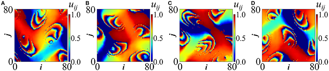
Figure 7. Spiral wave chimeras around a coherent core for random hierarchical connectivity in LIF model; potential profiles are depicted at four instances: (A) t = 3300 (B) t = 3360 (C) t = 3420 and (D) t = 3480 (in time units). Parameters are σ = 0.22 and T_r = 0.6. All other parameters are as in Figure 2A. Simulations start from random initial conditions. A related video is included in the Supplementary Material.

For larger values of T_r coherent double spots and stripe chimeras are formed, surrounded by the incoherent domains (Figure 8). In the top row of Figure 8 we can see the formation of a triple pattern (Figure 8A) composed by (i) a coherent stripe crossed by a traveling wave [57], (ii) an incoherent stripe surrounding the coherent region, while (iii) a third region consisting of traveling waves appears within the incoherent domain, at the top and bottom of the figure. The velocities of the traveling waves and the oscillator frequencies are different in the first and the third regions and this may support the idea of bistability. The presence of the incoherent region serves the purpose of continuity. Unlike the well known chimera patterns which is composed of two types of domains (coherent and incoherent), this is a curious chimera pattern which consists of three different domain types: coherent traveling waves with low velocity (region i), incoherent part (region ii) and coherent traveling waves with high velocity (region iii). The mean phase velocity distribution shows two maxima: one at the low frequencies which corresponds to the coherent domain and one in the high frequencies related to the high speed traveling waves. The intermediate ω values are attributed to the incoherent domain.

FIGURE 8

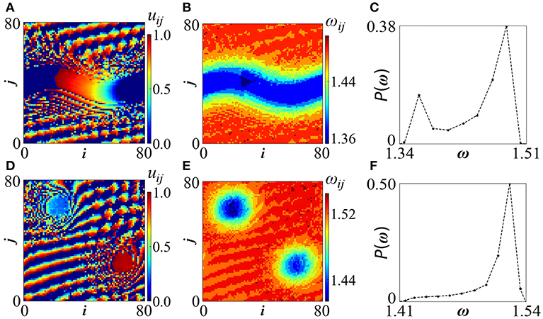
Figure 8. Random hierarchical connectivity in LIF model. Top row: Stripe chimera for parameters σ = 0.22, T_r = 2.0. (A) u_ij-profiles, (B) ω_ij-profiles and (C) distribution of ω-values. The P(ω) spectrum present two distinguishable maxima: one at the high ω-region which correspond to the traveling waves with short wavelength and one in the low ω-values associated with the stripe. Bottom row: Double coherent spot chimera for σ = 0.26 and T_r = 2.0. (D) u_ij-profiles, (E) ω_ij-profiles and (F) distribution of ω-values. The P(ω) spectrum presents only distinguishable maximum at the high ω-region which correspond to the traveling waves with short wavelength. A peak in the low ω-values in (F) is not observable because the extent of the two coherent spots [“blue” regions in (E)] is of similar size to the extent of the incoherent domains [“yellow” regions in (E)] and therefore a plateau appears. The dashed lines in (C,F) serve as eye guides. All other parameters are as in Figure 2A. Simulations start from random initial conditions. Other related images are available in the Supplementary Material.

By increasing the coupling strength, σ = 0.26, the stripe splits into two coherent spots, around which incoherent domains develop (Figure 8B). Again, the two incoherent domains are separated by spatial traveling patterns. Here the mean phase velocity distribution shows only a distinct maximum in the high frequencies which corresponds to the traveling waves. The two coherent spots have small sizes and their extent (size) is relatively small, not enough to produce a maximum in the low ω region in Figure 8F. Alternatively, the extent of “blue” regions in Figure 8E which characterize the coherent cores is similar to the extent of yellow regions which characterize the incoherent domains and therefore the spectrum in Figure 8F shows a plateau in the region of low mean phase velocities. The ω-profiles demonstrate that the coherent spots and the stripe acquire the lowest mean phase velocities, the incoherent domains have intermediate ω-values, while the traveling wave regions show the highest ω-values.

Related to the ω−profiles in the coherent domains (spots and stripe) we may assume, similarly to the Kuramoto phase oscillators, that the coupling term contribution in Equation (1a) reduces to zero because oscillators in the coherent domains have a phase difference of zero to their nonlocal neighbors. Unlike the Kuramoto model, in the LIF model the coherent domains present ω− values close (but not equal) to the uncoupled system. In the incoherent domains the coupling term is not negligible (because the oscillators in the nonlocal neighborhood have different phases) and for the coupling strength we use in this study we observe that ω_incoh > ω_coh.

Calculations of the local order parameter in the u_ij profile is often used to test synchronization in systems of coupled oscillators [29]. The local order parameter r_ij around oscillator (i, j) is defined as $r_{ij}=\frac{1}{n_c}\sum _{k,l}exp(i\varphi (k,l))$. The phase ϕ(k, l) of oscillator (k, l) is defined as ϕ(k, l) = [(2πu_kl)/u_th], so that ϕ varies between 0 and 2π. The sum runs over the n_c first neighbors of the oscillator (i, j). In the present study the immediate neighborhood is defined as a (3 × 3)-square around the oscillator (i, j), and therefore n_c = 8. The local order parameters are depicted in Figure 9A for the state in Figures 7A, 9B for the stripe of Figures 8A, 9C for the double coherent spots of Figure 8D. The profile of the local order parameter confirms the conclusions on the chimera profiles in all three cases, with lighter colors indicating phase coherence and darker colors phase incoherence.

FIGURE 9

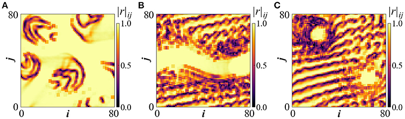
Figure 9. The local order parameter r_ij for (A) the spiral wave chimera as depicted in Figures 7A, (B) the stripe chimera of Figures 8A, (C) the double coherent spots of Figure 8D.

In particular for the case of the stripe and the double coherent spots (Figures 9B,C), the r_ij-values demonstrate coherence of the u_ij values in the regions of the stripe and the spots, respectively. To the best of our knowledge, these are new types of chimera manifested in 2D geometries, which allow freedom for coexistence of multiple stable domains with different oscillatory features in each domain.

5. Conclusions and Open Problems

In the present study we report on how details of the hierarchical connectivity matrix modify the emerging chimera patterns in 2D toroidal geometry. Using as working model the Leaky Integrate-and-Fire oscillator, we present numerical evidence (see Table 1) that traces of the hierarchical connectivity motif are demonstrated only for small values of the coupling strength σ (Figure 2). For large σ values, the exchange between the oscillating elements is strong, the dynamics develop fast and erratic motion or traveling patterns emerge which destroy the formation of hierarchical ordering within the incoherent domains of the chimera states. A complete list of our simulation results is outlined in Table 1.

The introduction of asymmetric (not rotationally invariant) coupling kernels, in the form of deterministic or random fractals, has induced spiral wave chimeras and traveling or erratically moving chimeras. In particular, for connectivity schemes with random hierarchical kernels and for low refractory period, we report a novel spiral wave chimera with a coherent core which is different from the spiral wave chimeras reported in the literature which rotate around incoherent cores. For larger values of the refractory period we also report a peculiar type of chimera which include three types of domains: coherent (in the form of coherent spots or stripes), incoherent and traveling waves. These chimera states are stable and emerge also for small values of the coupling strength. For symmetric hierarchical coupling and large system sizes spiral wave multichimeras are possible. These are composed by ordered spiral waves on the torus rotating around multiple cores consisting of asynchronous oscillators.

Regarding traveling chimera states, to study quantitatively their ω-profiles in future studies it could be useful to use a comoving frame, which moves with the velocity of the traveling pattern. This way one could extract the correct frequencies, since all nodes will be fixed either to the coherent or to the incoherent domains, without alternating between them.

From this study the rich variety of chimera patterns is evident, especially in 2D geometries, which give enough freedom for creation and stabilization of diverse forms. We have seen that by increasing the size of the system, e.g., from 81 × 81 to 243 × 243, it is possible to stabilize multichimera states, even for stochastic fractal connectivity. Apart from increasing the system size, other ways of pinning the traveling patterns (see e.g., Isele et al. [58] and Ruzzene et al. [59]) could be used in order to clarify the presence of hierarchical patterns in the ω− profile within the incoherent domains.

Another class of related problems concerns the dimensionality of the fractal kernels. In the present study flat fractals were considered with Hausdorff dimension ln 8/ln 3 ≈ 1.8928 as connectivity matrices. It would be interesting to consider kernels with different dimensionality and study the chimera patterns which are produced. Other open problems include the introduction of hierarchical connectivity in three-dimensions to explore the chimera patterns and other synchronization phenomena which emerge. Further extensions include the use of realistic connectivity schemes obtained directly from MRI images in order to address applications related to synchronization of brain neurons.

Data Availability

All data generated for this study can be found in the manuscript and the Supplementary Information.

Author Contributions

GA and AP formulated the problem and designed the study. GA performed the computations. Both authors discussed the results and contributed to writing the manuscript, read, and approved the final manuscript.

Funding

This work was supported by computational time granted from the Greek Research & Technology Network (GRNET) in the National HPC facility–ARIS–under project CoBrain3 (project ID: PR005014_taskp).

Conflict of Interest Statement

The authors declare that the research was conducted in the absence of any commercial or financial relationships that could be construed as a potential conflict of interest.

Acknowledgments

The authors acknowledge helpful discussions with N. Tsigkri-Desmedt and I. Koulierakis. The authors would like to thank the reviewers for pointing out many interesting aspects of this work.

Supplementary Material

The Supplementary Material for this article can be found online at: https://www.frontiersin.org/articles/10.3389/fams.2019.00035/full#supplementary-material

Figure S1. Depicts the distribution of ω values P(ω) of the oscillator which have local order parameter greater than 0.25 (these are about 90%).

Figure S2. Depicts the distribution of ω values P(ω) of the oscillators which have local order parameter less than 0.25.

Figure S3. Depicts the distribution of ω values P(ω) of the oscillators which have local order parameter greater than 0.5.

Figure S4. Depicts the distribution of ω values P(ω) of the oscillators which have local order parameter less than 0.5.

Video S1. Rotating fronts in synchronous background. Corresponds to Figure 7.

Video S2. Creation of 4 asynchronous sports with evolving internal structure. Corresponds to Figure 4.

Footnotes

1. ^https://github.com/gArgyropoulos/LIF_2D (2019).

2. ^Two videos related to Figures 4, 7 are added in the Supplementary Material (2019).

References

1. Kuramoto Y. Reduction methods applied to nonlocally coupled oscillator systems. In: Hogan SJ, Champneys AR, Krauskopf AR, di Bernado M, Wilson RE, Osinga HM, et al., editors. Nonlinear Dynamics and Chaos: Where Do We Go From Here? Boca Raton, FL: CRC Press (2002). p. 209–27.

Google Scholar

2. Kuramoto Y, Battogtokh D. Coexistence of coherence and incoherence in nonlocally coupled phase oscillators. Nonlinear Phenom Comp. (2002) 5:380.

Google Scholar

3. Abrams DM, Strogatz SH. Chimera states for coupled oscillators. Phys Rev B. (2004) 93:174102. doi: 10.1103/PhysRevLett.93.174102

PubMed Abstract | CrossRef Full Text | Google Scholar

4. Hagerstrom AM, Murphy TE, Roy R, Hövel P, Omelchenko I, Schöll E. Experimental observation of chimeras in coupled-map lattices. Nat Phys. (2012) 8:658. doi: 10.1038/nphys2372

CrossRef Full Text | Google Scholar

5. Martens EA, Thutupalli S, Fourrière A, Hallatschek O. Chimera states in mechanical oscillator networks. Proc Natl Acad Sci USA. (2013) 110:10563–67. doi: 10.1073/pnas.1302880110

PubMed Abstract | CrossRef Full Text | Google Scholar

6. Lazarides N, Neofotistos G, Tsironis GP. Chimeras in SQUID metamaterials. Phys Rev B. (2015) 91:054303. doi: 10.1103/PhysRevB.91.054303

CrossRef Full Text | Google Scholar

7. Gambuzza LV, Buscarino A, Chessari S, Fortuna L, Meucci R, Frasca M. Experimental investigation of chimera states with quiescent and synchronous domains in coupled electronic oscillators. Phys Rev E. (2014) 90:032905. doi: 10.1103/PhysRevE.90.032905

PubMed Abstract | CrossRef Full Text | Google Scholar

8. Tinsley MR, Nkomo S, Showalter K. Chimera and phase-cluster states in populations of coupled chemical oscillators. Nat Phys. (2012) 8:662–5. doi: 10.1038/nphys2371

CrossRef Full Text | Google Scholar

9. Wickramasinghe M, Kiss IZ. Spatially organized dynamical states in chemical oscillator networks: Synchronization, dynamical differentiation, and chimera patterns. PLoS ONE. (2013) 8:e80586. doi: 10.1371/journal.pone.0080586

PubMed Abstract | CrossRef Full Text | Google Scholar

10. Schmidt L, Schönleber K, Krischer K, García-Morales V. Coexistence of synchrony and incoherence in oscillatory media under nonlinear global coupling. Chaos. (2014) 24:013102. doi: 10.1063/1.4858996

PubMed Abstract | CrossRef Full Text | Google Scholar

11. Cherry EM, Fenton FH. Visualization of spiral and scroll waves in simulated and experimental cardiac tissues. N J Phys. (2008) 10:125016. doi: 10.1088/1367-2630/10/12/125016

CrossRef Full Text | Google Scholar

12. Rattenborg NC, Amlaner CJ, Lima SL. Behavioral, neurophysiological and evolutionary perspectives on unihemispheric sleep. Neurosci Biobehav Rev. (2000) 24:817–42. doi: 10.1016/S0149-7634(00)00039-7

PubMed Abstract | CrossRef Full Text | Google Scholar

13. Mormann F, Lehnertz K, David P, Elger CE. Mean phase coherence as a measure for phase synchronization and its application to the EEG of epilepsy patients. Phys D. (2000) 144:358–369. doi: 10.1016/S0167-2789(00)00087-7

CrossRef Full Text | Google Scholar

14. Mormann F, Kreuz T, Andrzejak RG, David P, Lehnertz K, Elger CE. Epileptic seizures are preceded by a decrease in synchronization. Epilepsy Res. (2003) 53:173. doi: 10.1016/S0920-1211(03)00002-0

PubMed Abstract | CrossRef Full Text | Google Scholar

15. Andrzejak RG, Rummel C, Mormann F, Schindler K. All together now: analogies between chimera state collapses and epileptic seizures. Sci Rep. (2016) 6:23000. doi: 10.1038/srep23000

PubMed Abstract | CrossRef Full Text | Google Scholar

16. Bansal K, Garcia JO, Tompson SH, Verstynen T, Vettel JM, Muldoon SF. Cognitive chimera states in human brain networks. Sci Adv. (2019) 5:eaau853. doi: 10.1126/sciadv.aau8535

PubMed Abstract | CrossRef Full Text | Google Scholar

17. Omelchenko I, Omel'chenko OE, Hövel P, Schöll E. When nonlocal coupling between oscillators becomes stronger: patched synchrony or multi-chimera states. Phys Rev B. (2013) 110:224101. doi: 10.1103/PhysRevLett.110.224101

CrossRef Full Text | Google Scholar

18. Omelchenko I, Provata A, Hizanidis J, Schöll E, Hövel P. Robustness of chimera states for coupled FitzHugh-Nagumo oscillators. Phys Rev E. (2015) 91:022917. doi: 10.1103/PhysRevE.91.022917

PubMed Abstract | CrossRef Full Text | Google Scholar

19. Schmidt A, Kasimatis T, Hizanidis J, Provata A, Hövel P. Chimera patterns in two-dimensional networks of coupled neurons. Phys Rev E. (2017) 95:032224. doi: 10.1103/PhysRevE.95.032224

PubMed Abstract | CrossRef Full Text | Google Scholar

20. Hizanidis J, Kanas V, Bezerianos A, Bountis T. Chimera states in networks of nonlocally coupled Hindmarsh-Rose neuron models. Int J Bifurcat Chaos. (2013) 24:1450030. doi: 10.1142/S0218127414500308

CrossRef Full Text | Google Scholar

21. Ulonska S, Omelchenko I, Zakharova A, Schöll E. Chimera states in networks of Van der Pol oscillators with hierarchical connectivities. Chaos. (2016) 26:094825. doi: 10.1063/1.4962913

PubMed Abstract | CrossRef Full Text | Google Scholar

22. Olmi S, Martens EA, Thutupalli S, Torcini A. Intermittent chaotic chimeras for coupled rotators. Phys Rev E. (2015) 92:030901. doi: 10.1103/PhysRevE.92.030901

PubMed Abstract | CrossRef Full Text | Google Scholar

23. Tsigkri-DeSmedt ND, Hizanidis J, Schöll E, Hövel P, Provata A. Chimeras in leaky integrate-and-fire neural networks: effects of reflecting connectivities. Eur Phys J B. (2017) 90:139. doi: 10.1140/epjb/e2017-80162-0

CrossRef Full Text | Google Scholar

24. Tsigkri-DeSmedt ND, Koulierakis I, Karakos G, Provata A. Synchronization patterns in Leaky Integrate-and-Fire neuron networks: merging nonlocal and diagonal connectivity. Eur Phys J B. (2018) 91:305. doi: 10.1140/epjb/e2018-90478-8

CrossRef Full Text | Google Scholar

25. Panaggio MJ, Abrams D. Chimera states: coexistence of coherence and incoherence in networks of coupled oscillators. Nonlinearity. (2015) 28:R67–R87. doi: 10.1088/0951-7715/28/3/R67

CrossRef Full Text | Google Scholar

26. Schöll E. Synchronization patterns and chimera states in complex networks: interplay of topology and dynamics. Eur Phys J Spec Top. (2016) 225:891–919. doi: 10.1140/epjst/e2016-02646-3

CrossRef Full Text | Google Scholar

27. Yao N, Zheng Z. Chimera states in spatiotemporal systems: theory and Applications. Int J Mod Phys B. (2016) 30:1630002. doi: 10.1142/S0217979216300024

CrossRef Full Text | Google Scholar

28. Majhi S, Bera BK, Ghosh D, Perc M. Chimera states in neuronal networks: a review. Phys Life Rev. (2018) 28:100–21. doi: 10.1016/j.plrev.2018.09.003

CrossRef Full Text | Google Scholar

29. Omel'Chenko OE. The mathematics behind chimera states. Nonlinearity. (2018) 31:R121. doi: 10.1088/1361-6544/aaaa07

CrossRef Full Text | Google Scholar

30. Omel'Chenko OE, Wolfrum M, Yanchuk S, Maistrenko YL, Sudakov O. Stationary patterns of coherence and incoherence in two-dimensional arrays of non-locally-coupled phase oscillators. Phys Rev E. (2012) 85:036210. doi: 10.1103/PhysRevE.85.036210

PubMed Abstract | CrossRef Full Text | Google Scholar

31. Panaggio MJ, Abrams D. Chimera states on a flat torus. Phys Rev B. (2013) 110:094102. doi: 10.1103/PhysRevLett.110.094102

PubMed Abstract | CrossRef Full Text | Google Scholar

32. Kundu S, Majhi S, Bera BK, Ghosh D, Lakshmanan M. Chimera states in two-dimensional networks of locally coupled oscillators. Phys Rev E. (2018) 97:022201. doi: 10.1103/Phys-RevE.97.022201

PubMed Abstract | CrossRef Full Text | Google Scholar

33. Totz JF, Rode J, Tinsley MR, Showalter K, Engel H. Spiral wave chimera states in large populations of coupled chemical oscillators. Nat Phys. (2018) 14:282–5. doi: 10.1038/s41567-017-0005-8

CrossRef Full Text | Google Scholar

34. Paul B, Banerjee T. Chimeras in digital phase-locked loops. Chaos. (2019) 29:013102. doi: 10.1063/1.5077052

PubMed Abstract | CrossRef Full Text | Google Scholar

35. Liu JZ, Zhang LD, Yue GH. Fractal dimension in human cerebellum measured by magnetic resonance imaging. Biophys J. (2003) 85:4041–6. doi: 10.1016/S0006-3495(03)74817-6

PubMed Abstract | CrossRef Full Text | Google Scholar

36. Katsaloulis P, Verganelakis DA, Provata A. Fractal dimension and lacunarity of tractography images of the human brain. Fractals. (2009) 17:181–9. doi: 10.1142/S0218348X09004284

CrossRef Full Text | Google Scholar

37. Expert P, Lambiotte R, Chialvo DR, Christensen K, Jensen HJ, Sharp DJ, et al. Self-similar correlation function in brain resting-state functional magnetic resonance imaging. J R Soc Int. (2011) 8:472–9. doi: 10.1098/rsif.2010.0416

PubMed Abstract | CrossRef Full Text | Google Scholar

38. Katsaloulis P, Ghosh A, Philippe AC, Provata A, Deriche R. Fractality in the neuron axonal topography of the human brain based on 3-D diffusion MRI. Eur Phys J B. (2012) 85:150. doi: 10.1140/epjb/e2012-30045-y

CrossRef Full Text | Google Scholar

39. Katsaloulis P, Hizanidis J, Verganelakis DA, Provata A. Complexity measures and noise effects on Diffusion Magnetic Resonance Imaging of the neuron axons network in the human brain. Fluct Noise Lett. (2012) 11:1250032. doi: 10.1142/S0219477512500320

CrossRef Full Text | Google Scholar

40. Hizanidis J, Panagakou E, Omelchenko I, Schöll E, Hövel P, Provata A. Chimera states in population dynamics: networks with fragmented and hierarchical connectivities. Phys Rev E. (2015) 92:012915. doi: 10.1103/PhysRevE.92.012915

PubMed Abstract | CrossRef Full Text | Google Scholar

41. Tsigkri-DeSmedt ND, Hizanidis J, Hövel P, Provata A. Multi-chimera states and transitions in the Leaky Integrate-and- Fire model with nonlocal and hierarchical connectivity. Eur Phys J Spec Top. (2016) 225:1149–64. doi: 10.1140/epjst/e2016-02661-4

CrossRef Full Text | Google Scholar

42. Sawicki J, Omelchenko I, Zakharova A, Schöll E. Chimera states in complex networks: interplay of fractal topology and delay. Eur Phys J Spec Top. (2017) 226:1883–92. doi: 10.1140/epjst/e2017-70036-8

CrossRef Full Text | Google Scholar

43. Chouzouris T, Omelchenko I, Zakharova A, Hlinka J, Jiruska P, Schöll E. Chimera states in brain networks: empirical neural vs. modular fractal connectivity. Chaos. (2018) 28:045112. doi: 10.1063/1.5009812

CrossRef Full Text | Google Scholar

44. Sawicki J, Omelchenko I, Zakharova A, Schöll E. Delay-induced chimeras in neural networks with fractal topology. Eur Phys J B. (2019) 92:54. doi: 10.1140/epjb/e2019-90309-6

CrossRef Full Text | Google Scholar

45. Argyropoulos G, Kasimatis T, Provata A. Chimera patterns and subthreshold oscillations in two-dimensional networks of fractally coupled leaky integrate-and-fire neurons. Phys Rev E. (2019) 99:022208. doi: 10.1103/PhysRevE.99.022208.

PubMed Abstract | CrossRef Full Text | Google Scholar

46. Brunel N, van Rossum MCW. Lapicque's 1907 paper: from frogs to integrate-and-fire. Brain Res Bull. (1999) 50:303–4.

Google Scholar

47. Abott LF. Lapicque's introduction of the integrate-and-fire model neuron (1907). Biol Cybernet. (2007) 97:337–9.

Google Scholar

48. Kuramoto Y. Collective synchronization of pulse-coupled oscillators and excitable units. Phys D. (1990) 50:15–30.

Google Scholar

49. Luccioli S, Politi A. Irregular collective behavior of heterogeneous neural networks. Phys Rev E. (2010) 105:158104. doi: 10.1103/PhysRevLett.105.158104

PubMed Abstract | CrossRef Full Text | Google Scholar

50. Olmi S, Politi A, Torcini A. Collective chaos in pulse-coupled neural networks. Eur Lett. (2010) 92:60007. doi: 10.1209/0295-5075/92/60007

CrossRef Full Text | Google Scholar

51. Ullner E, Politi A, Torcini A. Ubiquity of collective irregular dynamics in balanced networks of spiking neurons. Chaos. (2018) 28:081106. doi: 10.1063/1.5049902

PubMed Abstract | CrossRef Full Text | Google Scholar

52. Kasimatis T, Hizanidis J, Provata A. Three-dimensional chimera patterns in networks of spiking neuron oscillators. Phys Rev E. (2018) 97:052213. doi: 10.1103/PhysRevE.97.052213

PubMed Abstract | CrossRef Full Text | Google Scholar

53. Mandelbrot BB. The Fractal Geometry of Nature. San Francisco, CA: W.H. Freeman and Co. (1982).

Google Scholar

54. Takayasu H. Fractals in Physical Science. Manchester; New York, NY: Manchester University Press (1991).

Google Scholar

55. Omel'Chenko OE, Wolfrum W, Knobloch E. Stability of spiral chimera states on a torus. SIAM J Appl Dynam Syst. (2018) 17:97–127. doi: 10.1137/17M1141151

CrossRef Full Text | Google Scholar

56. Martens S, Ryll C, Löber J, Tröltzsch F, Engel H. Control of Traveling Localized Spots. (2018). Available online at: https://arxivorg/abs/170304246 (accessed September 20, 2018).

Google Scholar

57. Nkomo S, Tinsley MR, Showalter K. Chimera and chimera-like states in populations of nonlocally coupled homogeneous and heterogeneous chemical oscillators. Chaos. (2016) 26:094826. doi: 10.1063/1.4962631

PubMed Abstract | CrossRef Full Text | Google Scholar

58. Isele T, Hizanidis J, Provata A, Hövel P. Controlling chimera states: the influence of excitable units. Phys Rev E. (2016) 93:022217. doi: 10.1103/PhysRevE.93.022217

PubMed Abstract | CrossRef Full Text | Google Scholar

59. Ruzzene G, Omelchenko I, Schöll E, Zakharova A, Andrzejak RG. Controlling chimera states via minimal coupling modification. Chaos. (2019) 29:0511031. doi: 10.1063/1.5097570

PubMed Abstract | CrossRef Full Text | Google Scholar