Identifying Arguments of Space-Time Fractional Diffusion: Data-Driven Approach

1. Introduction

Technological advances ranging from an impressive improvement in the sensing and computational resources to the enhancement in data storage play a prominent role in offering researchers' new directions to investigate unknown or poorly understood phenomena and boost numerous scientific areas (e.g., neuroscience, synthetic and system biology, finance, anthropology, and political sciences). This impact on all sciences is likely to persist with the booming advances in data science (DS), machine learning (ML), and artificial intelligence (AI) [1–4]. Apart from the impressive contribution of AI in pattern recognition (e.g., images) and language processing, nowadays AI and data science are contributing to several developing scientific fields (e.g., the discovery of unwanted effects of drugs and drug repositioning [5, 6]). For example, one can consider the problem of “Lamisil” drug used for the treatment of skin infections, which caused deaths and other liver reactions after being on the market for years. Although it was found that the drug is behind the TBF-A generation, which has toxicological effects, it was not possible to explain how the drug boosts the TBF-A formation. In 2018, a deep learning-based investigation identified the pathways leading to TBF-A formation [5]. The process of TBF-A formation could not be identified before launching the product on the market due to its complicated mechanism and limited information on its manifestations. Such a discovery can have a primordial role in drug discovery and development by pharmaceutical industries and startups working in drug discovery (e.g., Kebotix, Deep Genomics).

Furthermore, AI has been recently considered as a useful analysis and discovery tool in medicine and healthcare. For instance, computer scientists and radiologists incorporated ML and AI techniques into the radiological examination in order to provide better results in medical imaging [7] and to detect early signs of diseases. Indeed, convolutional neural networks based approaches enabled the analysis of three dimensional MRI images and the identification of symptoms of Alzheimer's disease [8]. Similarly, AI-based investigation provided new approaches for quantifying the risk of autism [9]. It is also worth mentioning that AI has also been introduced in ophthalmology [10]. Beyond the medical field, reinforcement learning has been recently used in meteorology in order to study the climate [11, 12]. Consequently, we are witnessing a paradigm shift in mining and understanding real-world problems, as a variety of late innovations are based on applying ML algorithms to analyze and characterize high-dimensional experimental data.

Despite the tremendous boost that is provided by the ML and AI for the analysis of static data through identifying the statistical interdependence between components of a system of interest, there is little to say about analyzing dynamical processes from big data and uncertainty quantification for large-scale complex systems. Specifically, ML has a limiting ability in deciphering the physical driving laws and governing equations from multi-modal heterogeneous, scarce, and/or noisy time-series data associated with complex systems exhibiting multi-scale and multi-physics spatiotemporal evolution. These multi-scale and multi-physics spatiotemporal characteristics that occur in physics, biology, chemistry, neuroscience, and even geology, are usually encoded through (fractional or integer order) partial differential equations (PDEs) with possibly uncertain parameters. These PDEs are derived from conservation laws on energy, momentum, or electric charge (e.g., diffusion equation, Maxwell's equations, Navier-Stokes equations, Schrodinger equations). However, a plethora of complex systems from biology, neuroscience, or finance have numerous hidden interaction mechanisms, and the derivation of the PDEs describing their evolution is unknown. In the big data era, we witness new opportunities for data-driven discoveries of potentially new physical phenomena and new physics laws (or rules). Consequently, one may ask the following fundamental question: Can we learn a PDE model from a given set of time-series measurements and perform accurate, efficient, and robust predictions using this learned model? This question has motivated researchers to develop methods for estimating PDE parameters using numerical solutions of PDEs [13, 14] (which requires careful parameterizations and high computational cost), Bayesian approaches [15], and a two-state approach [16–19] where the parameters of the PDEs are estimated via least squares. However, exploiting the higher-order statistics of the measurements, which can characterize the rare events for a robust understanding of complex systems, and determining whether fractional or integer order PDEs together with their corresponding parameters govern the observations, has not been addressed.

Diffusion is one of the fundamental mechanisms used for analyzing the transport of particles, and a common example of a diffusion process is the Brownian motion. Chaotic motion of a particle characterizes the latter process, and it can be modeled by a random walk such that the mean square displacement follows the diffusing scaling < (ΔX)² >~ t (where < . > designates the mean). Furthermore, diffusion is a principal concept that explains many natural and scientific/technological phenomena (e.g., particles motion [20], DNA and cellular processing [21–24], microbial communities [25], brain activity [26], physiological complexity and cyber-physical systems modeling [27–29]), neuron spikes [30]. The focus on analyzing complex systems led to studying anomalous diffusion [31–43] to decipher complex system properties (e.g., long-range memory, higher-order correlations, ergodicity breaking measured as a discrepancy between the long time-averaged mean squared displacement and the ensemble-averaged mean squared displacement). The anomalous diffusion has been shown to be able to describe complex fluid dynamics [44, 45], biological systems [46–48], transport [49], dynamics in fractal structures [50–52], and economics [53]. Contrary to random walks processes describing classical diffusion (e.g., Brownian motion), the particle possesses an internal memory that leads to a non-stationary motion, where the mean square displacement is heavy-tailed < (ΔX)² >~ t^β (β is a parameter that is related to the memory of a particle).

The principal purpose for studying anomalous diffusion is to take into account complex/non-trivial behavior of the motion of particles usually found in transport processes in disordered and complex systems. From a phenomenological perspective, the anomalous diffusion can be better understood by recalling the assumptions made by Einstein [20] on defining the normal diffusion: the motion of the Brownian particles are independent (valid for small concentrations), there exist a small time scale during which the particle displacements are statistically independent (i.e., a Markovian behavior), and the particle displacements at these time scales correspond to a mean free path distributed symmetrically in positive or negative directions (i.e., a symmetric Gaussian statistical behavior). In contrast, anomalous diffusion generalizes the normal diffusion framework by removing one or more of such requirements on either Markovian or Gaussian behavior [42, 43]. In the literature, there are many methods used to analyze anomalous diffusion, mainly generalized Langevin equation [54, 55], thermodynamics [56, 57] and in this article, we concentrate our analysis on the discussion of incorporating fractional derivatives into PDEs to model anomalous diffusion. In fact, the mathematical description of anomalous diffusion involves a power law expression of the mean square displacement as a function of time. It often relies on fractional-order derivatives acting on either space or time components of a PDE [29, 42, 43]. Indeed, modeling anomalous diffusion via fractional diffusion equation (i.e., PDE) can be provided by the master equation for continuous time random walk, and the solutions of the fractional diffusion equation can be interpreted as spatial probability densities evolving in time, related to self-similar stochastic process encoding the long-range memory property [58]. For instance, the anomalous diffusion of a particle subject to an external non-linear force and a thermal bath is described in Metzler et al. [59] through a fractional Fokker-Planck equation. Here, the time-fractional Riemann-Liouville derivative models the long-range memory effects characteristic to anomalous diffusion in random environments and chaotic Hamiltonian systems [59]. More generally, the anomalous diffusion has been successfully modeled by a space-time fractional diffusion equation that assumes that the process has memory (i.e., time-fractional derivative) as well as being non-local (space-fractional derivative). More recently, a comprehensive analysis of the higher-order moments associated with the amplitude fluctuations of the time-averaged mean square displacement for an anomalous diffusion model demonstrated that the skewness and kurtosis can improve the estimation of the anomalous diffusion exponent and can help at classifying the anomalous stochastic processes [60].

Despite the significant body of work on anomalous diffusion models, finding the exact parameters of the corresponding governing PDE is not a trivial task. In this context, given a spatiotemporal dataset, we aim to develop an efficient algorithm for estimating the parameters of the generalized fractional-order PDE that models the dynamics of the process under investigation. Consequently, by identifying these parameters, one can also investigate the physical rules modeled by the PDE. In the results section, we analyze two types of PDEs and discuss algorithmic approaches to determine their parameters from the time-series data. We also provide a simulation study where we verify the correctness and effectiveness of the proposed algorithmic approaches on deriving the exact parameters using synthetic trajectories generated from the PDE model.

2. Data-Driven Approach for Analyzing Anomalous Diffusion

2.1. Space-Time Fractional Diffusion Equation

The space-time fractional diffusion equation has been proposed in previous works as a mathematical model to analyze anomalous diffusion [34, 61–65]. In a nutshell, the space-time fractional diffusion equation in (1) consists of a fractional Riesz-Feller derivative of the order α > 0 (space-derivative) that encodes the space variations and a fractional Caputo derivative of the order β > 0 (time-derivative) that measures the time variations. To better generalize, we also consider the skewness factor in the space derivative of the diffusion equation. Hence, the space-time fractional diffusion equation is defined as

$\begin{array}{ll}{}_t{{D}}_{*}^{\beta }u(x,t)=D{\times }_x{{D}}_{\theta }^{\alpha }u(x,t),\forall x\in ℝ,\forall t\in {ℝ}^{+},& (1)\end{array}$

where the operators ${}_x{{D}}_{\theta }^{\alpha }$ and ${}_t{{D}}_{*}^{\beta }$ designate the fractional Riesz-Feller derivative of order α and skewness θ [66], and the Caputo time-fractional derivative of order β [67], respectively¹. The parameter D denotes the generalized diffusion coefficient. The parameters α, β and θ satisfy the following constraints, 0 < α ≤ 2, 0 < β ≤ 1 and |θ| ≤ min{α, 2 − α}.

Given a set of time-series trajectories that record the evolution of particles or agents that exhibits anomalous diffusion modeled by Equation (1), without prior knowledge about the parameters of the space-time fractional diffusion equation, our goal is to use the dataset available to retrieve the exact fractional PDE that generates the given time-series. Toward this end, we develop a mathematical framework where the parameter and mathematical (operator) expression identification task is defined as a regression problem (Figure 1). Indeed, the regression is formulated as a least squares problem, where the minimization involves the theoretical and the empirical statistical (higher order) moments (i.e., specifically the absolute moments). The choice of the statistical moments for performing the regression is convenient because we could derive its closed form expressions just from the generalized fractional PDE given in Equation (1). For the given time-series data, X_n(t), 1 ≤ n ≤ N, where N denotes the total number of trajectories, the time empirical moments are defined as follows

$\begin{array}{ll}{M}_t^{\delta }=\frac{1}{N}{\displaystyle \sum _{n=1}^N}|X_n(t){|}^{\delta },S_t^{\delta }=\frac{1}{N}{\displaystyle \sum _{n=1}^N}{X}_n{(t)}^{\langle \delta \rangle },& (2)\end{array}$

where x^〈δ〉 denotes the signed absolute δ-th power of x and x^〈δ〉 = |x|^δsign(x). The time-dependent absolute moment of the data generated according to the fractional PDE in (1) is given by the following result.

FIGURE 1

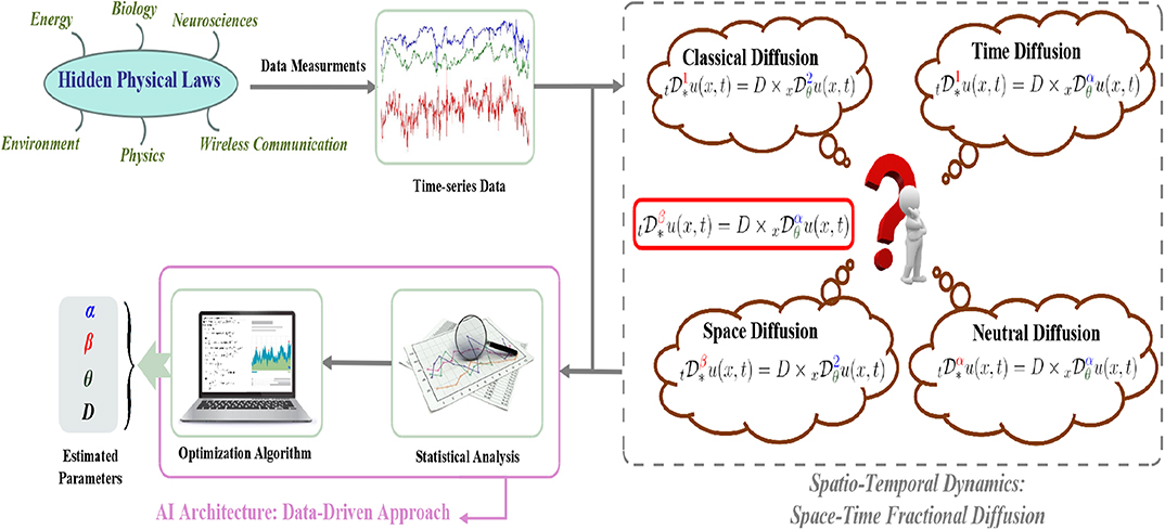
Figure 1. Flowchart showing an AI architecture used to uncover hidden patterns governing complex phenomena: a data-driven based approach to estimate the parameters of the space-time fractional diffusion equation from spatiotemporal dynamics.

Proposition 1. The time-dependent absolute moment of the order δ with 0 < δ < α is written as follows

$\begin{array}{ll}𝔼[|X(t){|}^{\delta }]=t^{\delta \frac{\beta }{\alpha }}{D}^{\frac{\delta }{\alpha }}\times \frac{\Gamma (1-\frac{\delta }{\alpha })\Gamma (1+\frac{\delta }{\alpha })cos(\frac{\delta \pi \theta }{2\alpha })}{\Gamma (1-\delta )\Gamma (1+\delta \frac{\beta }{\alpha })cos(\frac{\delta \pi }{2})},& (3)\end{array}$

where Γ(·) designates the gamma function.

To find the parameters of the fractional PDE in (1), we rely on analyzing the higher order moments and minimize the quadratic error between the theoretical and the empirical absolute higher order moments. However, due to the non-linear non-convex expression stated in the Equation (3), such a regression problem is non-trivial and it is non-trivial to provide the theoretical guarantees about the convergence of a multi-dimensional optimization algorithm used to solve the problem in one-shot. To tackle the non-convexity, we aim to approach the parameters estimation via multi-step optimization. For obtaining additional information from the data, we also derive the signed absolute as in the following result.

Proposition 2. The time-dependent signed absolute moment of the order δ with 0 < δ < α is written as follows

$\begin{array}{ll}𝔼[X{(t)}^{\langle \delta \rangle }]=-t^{\delta \frac{\beta }{\alpha }}{D}^{\frac{\delta }{\alpha }}\times \frac{\Gamma (1-\frac{\delta }{\alpha })\Gamma (1+\frac{\delta }{\alpha })sin(\frac{\delta \pi \theta }{2\alpha })}{\Gamma (1+\delta \frac{\beta }{\alpha })\Gamma (1-\delta )sin(\frac{\delta \pi }{2})}.& (4)\end{array}$

We refer the reader to the Supplementary Materials for the proofs of the above Propositions. Using the above results, the estimation of parameters is detailed in the following section.

2.2. Parameter Estimation

Absolute Moments Approach: Starting from a dataset containing N independent trajectories (realizations of the Equation (1) with unknown parameters) sampled uniformly at times {t₁, t₂, …, t_L}, we aim at estimating the actual parameters of the Equation (1) via a moments-based approach, i.e., determining the parameters using empirical moments and the theoretical expressions. Thus, the proposed scheme to find the parameters is mainly a two-step approach, regression over time on one hand and over space on the other hand. The method is summarized as follows.

For a given order δ, the log of absolute moments in Equation (3) varies as

$\begin{array}{ll}log(𝔼[|X(t){|}^{\delta }])=\delta \frac{\beta }{\alpha }log(t)+C_1,& (5)\end{array}$

where C₁ does not depend on t. Using the estimated empirical moments from Equation (2), we replace the theoretical moments with the empirical values in the Equation (5). The parameter ratio β/α can then be estimated by performing linear regression of log(t_l) vs. $log(M_{t_l}^{\delta })$ using a total of L points (i.e., l = 1, 2, …, L). It is worthwhile to note that the precision in estimation of β/α can be improved upon using multiple values of moment exponent δ for increasing the total diverse points in linear regression. For example, a set Δ = {δ₁, δ₂, …, δ_K} can be used for having K × L diverse points for linear regression by repeating the Equation (5) with different δ_k. Hence, we can make a trade-off between space and time, i.e., enlarging the cardinality of Δ when the available time-series are short, in other words when L is small.

Next, we use the results of Proposition 1 and 2 to get the ratio of 𝔼[|X(t)|^δ] and 𝔼[X(t)^〈δ〉] as the following ratio r

$\begin{array}{l}r=\frac{𝔼[X{(t)}^{\langle \delta \rangle }]}{𝔼[|X(t){|}^{\delta }]}=-\frac{tan(\frac{\pi \delta \theta }{2\alpha })}{tan(\frac{\pi \delta }{2})}.\end{array}$

Upon replacing the theoretical moments with the ones derived in Equation (2) we can invert the tangent function to have the ratio θ/α. In addition, although the ratio r is independent of time t, the empirical ratio of the data will possibly not be a constant across time. We therefore, replace r with time average of the ratio of $S_{t_l}^{\delta }$ and $M_{t_l}^{\delta }$ as $\overline{S_{t_l}^{\delta }/M_{t_l}^{\delta }}$. From section 2.1, we know that the parameter θ is constrained as |θ| ≤ min(α, 2 − α), therefore, we have |θ/α| ≤ 1. Next, we define the following function

$\begin{array}{l}{w}_L(x)=\{\begin{array}{cc}-1& x<-1\\ x& -1\le x\le 1\\ 1& x>1\end{array}.\end{array}$

Finally, the ratio of parameters θ and α can now be written as

$\begin{array}{ll}\frac{\theta }{\alpha }=w_L\left(-\frac{2}{\pi \delta }arctan\left(tan\left(\frac{\pi \delta }{2}\right)\overline{\left(\frac{S_{t_l}^{\delta }}{M_{t_l}^{\delta }}\right)}\right)\right).& (6)\end{array}$

As argued before, to improve the precision of the estimation, we can add diversity by having a set of moment exponents Δ = {δ₁, δ₂, …, δ_K}. For each δ_k ∈ Δ (where k = 1, 2, …, K), we use the Equation (6) to obtain ${\widehat{(\theta /\alpha )}}_k$, and finally obtain the estimated ratio of parameters as $\widehat{(\theta /\alpha )}=\frac{1}{K}{\sum }_{k=1}^K{\widehat{(\theta /\alpha )}}_k$.

The absolute moments of order δ from Proposition 1 can be re-written as follows

$\begin{array}{l}\frac{𝔼[|X(t){|}^{\delta }]}{t^{\delta \frac{\beta }{\alpha }}}=D^{\frac{\delta }{\alpha }}\times \frac{\Gamma (1-\frac{\delta }{\alpha })\Gamma (1+\frac{\delta }{\alpha })cos(\frac{\delta \pi \theta }{2\alpha })}{\Gamma (1-\delta )\Gamma (1+\delta \frac{\beta }{\alpha })cos(\frac{\delta \pi }{2})}\\ =D^{\frac{\delta }{\alpha }}\times \frac{\frac{\pi \delta }{\alpha }}{sin(\frac{\pi \delta }{\alpha })}\times \frac{cos(\frac{\pi \delta \theta }{2\alpha })}{\Gamma (1-\delta )\Gamma (1+\frac{\delta \beta }{\alpha })cos(\frac{\pi \delta }{2})}.\end{array}$

Therefore, for the given value of the order δ = δ_k, the estimation of α and diffusion coefficient D can be written as the following non-linear equation

$\begin{array}{l}{C}_k=\frac{\Gamma (1-{\delta }_k)\Gamma (1+\frac{{\delta }_k\beta }{\alpha })cos(\frac{\pi {\delta }_k}{2})}{cos(\frac{\pi {\delta }_k\theta }{2\alpha })}\times \frac{𝔼[|X(t){|}^{{\delta }_k}]}{t^{{\delta }_k\frac{\beta }{\alpha }}}\\ =D^{\frac{{\delta }_k}{\alpha }}\times \frac{\frac{\pi {\delta }_k}{\alpha }}{sin(\frac{\pi {\delta }_k}{\alpha })}.& (7)\end{array}$

To solve the non-linear equation in (7) for α and D, we use non-linear least squares method (trust region reflective method). The input variables to the non-linear optimization are the values of order δ ∈ Δ, where Δ = {δ₁, δ₂, …, δ_K}. Formally, the optimization problem is written as follows.

$\begin{array}{ll}\{\widehat{D},\widehat{\alpha }\}={\displaystyle \underset{\alpha ,D}{\text{argmin}}}{\displaystyle \sum _{k=1}^K}{\left|D^{\frac{{\delta }_k}{\alpha }}\times \frac{\frac{{\delta }_k\pi }{\alpha }}{sin(\frac{{\delta }_k\pi }{\alpha })}-C_k\right|}^2.& (8)\end{array}$

We note that the values of C_k can be efficiently estimated by first performing the linear regression of $t^{\delta \frac{\beta }{\alpha }}$ vs 𝔼[|X(t)|^δ] with the condition of zero intercept, and then substituting the ratio (slope of the linear regression) in Equation (7). The optimization problem in (8) is non-convex, therefore, the global optimum solution is not guaranteed by the solvers. Note that, in some scenarios, we may have a prior knowledge about boundaries of the parameter α (i.e., α_min ≤ α ≤ α_max). Thus, we solve the constrained optimization problem.

Finally, the values of β and θ can be estimated upon estimating α, as we already have the ratios β/α and θ/α from Equation (5) and Equation (6), respectively. The approach described is summarized as Algorithm 1.

ALGORITHM 1

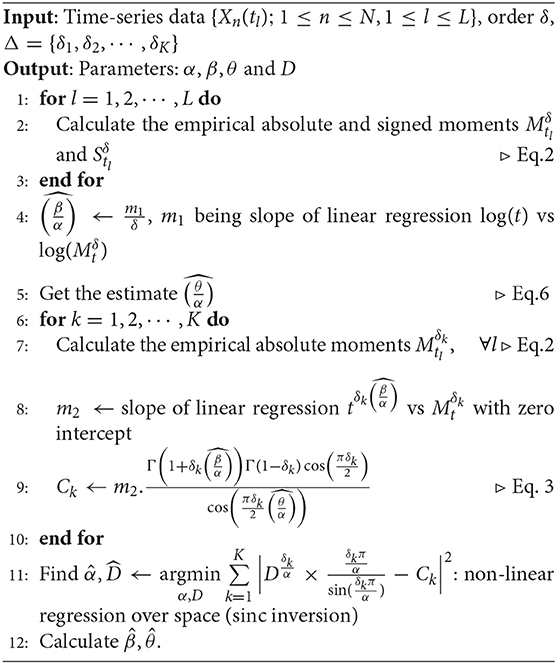
Algorithm 1. Space-Time Fractional Diffusion: Parameters Estimation

Remark: Note that for α ≠ 2, when the order δ is close to the boundary values, the theoretical absolute moment goes to +∞. However, the empirical one is finite, so in order to have a small error associated to the estimated parameters, we choose the order δ to be far enough from the end points of allowed region. Notice that, the value of α is unknown while the condition −min{α, 1} < ℜ(δ) < α is dependent of it, so assuming an α_min as lower bound for α is rational. We note that the Algorithm 1 is dependent upon the solution of non-linear non-convex optimization problem in (8), and therefore, convergence to the global solution is not guaranteed. Also, we need to provide an input set Δ such that the absolute and signed moments are computable for unknown α. The choice of Δ has to be made by having some idea about lower bound of the α parameter. To take care of these two issues together, we next present an alternative approach in which we do not require non-linear optimization as well as do not require to have the knowledge of Δ set.

Log Absolute Moments Approach: In this subsection, we rely on the moments of log absolute values of the trajectories. Similar to absolute moments with order δ, the log absolute moments can be computed as we present in the following results.

Proposition 3. The time-dependent expected log absolute value of X(t) is written as follows

$\begin{array}{ll}𝔼[log\left|X(t)\right|]=\frac{\beta }{\alpha }log(t)+\frac{log(D)}{\alpha }+\gamma \left(\frac{\beta }{\alpha }-1\right),& (9)\end{array}$

where γ is the Euler-Mascheroni constant.

Next, the variance of the log absolute values of the trajectories can be written as the following results.

Proposition 4. The variance of log absolute value of X(t) is written as follows

$\begin{array}{ll}\text{var}(log\left|X(t)\right|)=\frac{{\pi }^2}{6}\left(\frac{1}{{\alpha }^2}+\frac{1}{2}\right)-{\left(\frac{\pi \theta }{2\alpha }\right)}^2.& (10)\end{array}$

It is interesting to note that the variance is independent of time as well as a function of α and θ/α. We exploit this feature of the variance to obtain an estimate of the α with the ratio θ/α known. Hence, the need for performing non-linear optimization in Algorithm 1 is omitted. We also write the second moment of the log absolute values in the following result.

Proposition 5. The time-dependent expected square of log absolute value of X(t) is written as follows

$\begin{array}{ll}𝔼[{(log\left|X(t)\right|)}^2]=\frac{{\beta }^2}{{\alpha }^2}{log}^2(t)+2\frac{\beta \gamma }{\alpha }\left(\frac{\beta }{\alpha }-1\right)log(t)+c,& (11)\end{array}$

where $c=\frac{{\pi }^2}{6}\left(\frac{1}{{\alpha }^2}+\frac{1}{2}\right)-{\left(\frac{\pi \theta }{2\alpha }\right)}^2+{\left(\frac{log\left(D\right)}{\alpha }+\gamma \left(\frac{\beta }{\alpha }-1\right)\right)}^2+\frac{{\pi }^2}{6{\alpha }^2}(1-{\beta }^2)$, and γ is the Euler-Mascheroni constant.

The proof of the Propositions 3, 4, and 5 are provided in the Supplementary Materials. Using the above results for log absolute values, we now present the second approach to estimate the parameters of the space-time fractional PDE in (1).

We proceed similarly to the first approach of the δ order absolute moments, however, now equating the theoretical and empirical expressions of the log absolute moments. The empirical log absolute moments are written as

$\begin{array}{l}{L}_t^{(1)}=\frac{1}{N}{\displaystyle \sum _{n=1}^N}log|X_n(t)|,\\ L_t^{(2)}=\frac{1}{N}{\displaystyle \sum _{n=1}^N}log|X_n(t){|}^2,\\ \overline{\text{var}(log\left|X(t)\right|)}=\frac{1}{N-1}{\displaystyle \sum _{n=1}^N}{\left(log|X_n(t)|-L_t^{(1)}\right)}^2.& (12)\end{array}$

The parameter ratio β/α is estimated by performing the linear regression of log(t) vs $L_t^{(1)}$. The slope of the regression output is the estimated ratio $\widehat{(\beta /\alpha )}$. Next, the ratio of the parameters θ and α is estimated using the same approach as described previously in Equation (6).

We note that upon having an estimate of the parameter ratio $\widehat{\theta /\alpha }$, the variance is one-to-one function of α since α ≥ 0. Therefore, on substituting the value of $\widehat{\theta /\alpha }$ in Equation (10) we compute the value of $\hat{\alpha }$. Finally, with $\hat{\alpha }$ and $\widehat{\beta /\alpha }$ known, the value of diffusion coefficient is estimated from the intercept of the linear regression of log(t) vs $L_t^{(1)}$ as $\hat{D}$. The above described approach is summarized as an algorithmic strategy in Algorithm 2.

ALGORITHM 2

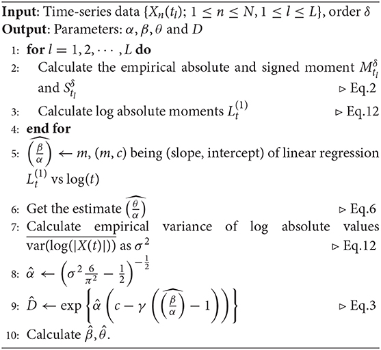
Algorithm 2. Space-Time Fractional Diffusion: Parameters Estimation

It should be noted that the approach utilizing log absolute moments does not require a predefined set of order values Δ. In addition, this does not suffer from the convergence issues as there is no non-linear non-convex optimization involved.

Note: The estimated parameters in both algorithms are not guaranteed to be optimal. For example, it is not straightforward to guarantee maximum likelihood sense as solving maximum likelihood involves solution to non-convex problem. We evaluate the efficiency of the both algorithms in the following section.

3. Experimental Results

As we described previously, both algorithms depend mainly on the statistical absolute moments, statistical signed absolute moments and the expected log absolute value of the process X(t). For this reason, we first start by validating the theoretical expressions derived in Equations (3), (4) and (9). We consider different scenarios (normal diffusion equation, neutral diffusion equation [68–71], space diffusion equation [71], and time diffusion equation [71]). In these experiments, we generate synthetic data corresponding to N = 100 trajectories simulated according to the diffusion model under study with a generalized diffusion coefficient D = 1. Note that the data generation procedure is presented in details in the Supplementary Material. In Figure 2, we present panel of 4 × 3 plots where we refer by a row the scenario considered (normal, time, space, neutral diffusion) and we plot the statistical absolute moments, statistical signed absolute moments and the expected log absolute value of the process X(t) for an order δ = 0.001 vs. time in the columns. The signed moment deviates a little from the theoretical expression for some scenarios, due to lack of sufficient samples. For the particular case of Figure 2E, we observe that there is nearly perfect match with the theoretical expression. The reason being, in this case, the parameters α = θ, hence the trajectories are generated from a negatively skewed alpha-stable distribution, therefore X(t) ≤ 0 ∀t. We note that a similar situation happens when we have the parameters α = −θ. In this case, we have a positive skewed alpha distribution, and therefore, X(t) ≥ 0∀t. In all scenarios, we can observe that the empirical statistical moments match perfectly the theoretical ones in all scenarios. This result confirms our theoretical derivations and motivates us to move forward with this approach.

FIGURE 2

Figure 2. The time-dependent theoretical and empirical absolute moments and signed absolute moments of order δ = 0.001, the time-dependent theoretical and empirical expected log absolute for the following four types of diffusion models: (A–C) Normal diffusion equation, (D–F) Neutral diffusion equation, (G–I) Space fractional diffusion equation, (J–L) Time fractional diffusion equation.

3.1. Parameters Estimation of Synthetic Data

In this experiment, we validate the proposed approach using artificially generated spatiotemporal data according to the PDE model presented in Equation (1). More precisely, we use the above-mentioned schemes (Algorithm 1 and Algorithm 2) to retrieve the parameters (α, β, θ and D) used during the data generation step. Figures 3–5 summarize several experiments done for different diffusion models (classical, neutral, space, and time diffusion), where we assume a set of combination of α, β and θ parameters for a generalized diffusion coefficient D = 1, 2 and D = 5, respectively. In each figure we present a panel of 4 × 4 different plots where a row represents the type of diffusion considered and columns 1, 2, 3 and 4 designate the parameters α, β, θ and D, respectively. In each of the sub-figure, we plot the estimated parameter using both algorithms (blue line for Algorithm 1 and the black line for Algorithm 2) vs. the number of trajectories considered during the estimation process. We also plot the true value as a red line, and a narrow interval around the true value using black dashed lines. The presented blue and gray shaded regions represent the standard deviation for the estimated parameters associated to Algorithm 1 and Algorithm 2, respectively. All sub-figures in Figures 3–5 show that the proposed schemes are doing well in all scenarios where we are able to retrieve the exact set of parameters α, β, θ and D with a small/negligible error². Also, we can see how the standard deviation of the estimated parameters decreases as the number of trajectories increases. Furthermore, we can remark that Algorithm 2 is performing slightly better than Algorithm 1 in terms of rate of convergence. Although the variance is quite high when fewer trajectories are considered, we remark that in some scenarios we can get good estimates of the parameters even with reduced number of trajectories.

FIGURE 3

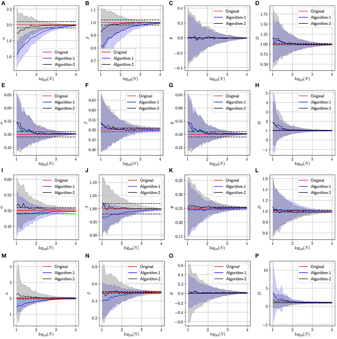
Figure 3. Determining the parameters of the space-time fractional diffusion via the two proposed algorithms while varying the number of trajectories and the generalized diffusion coefficient D = 1. The dotted line indicate 2% error tube around the original parameter value in the red: (A–D) Normal diffusion equation (α = 2, β = 1, θ = 0), (E–H) Neutral diffusion equation (α = 0.5, β = 0.5, θ = 0.5), (I–L) Space fractional diffusion equation (α = 0.5, β = 1, θ = 0.25), (M–P) Time fractional diffusion equation (α = 2, β = 0.5, θ = 0).

FIGURE 4

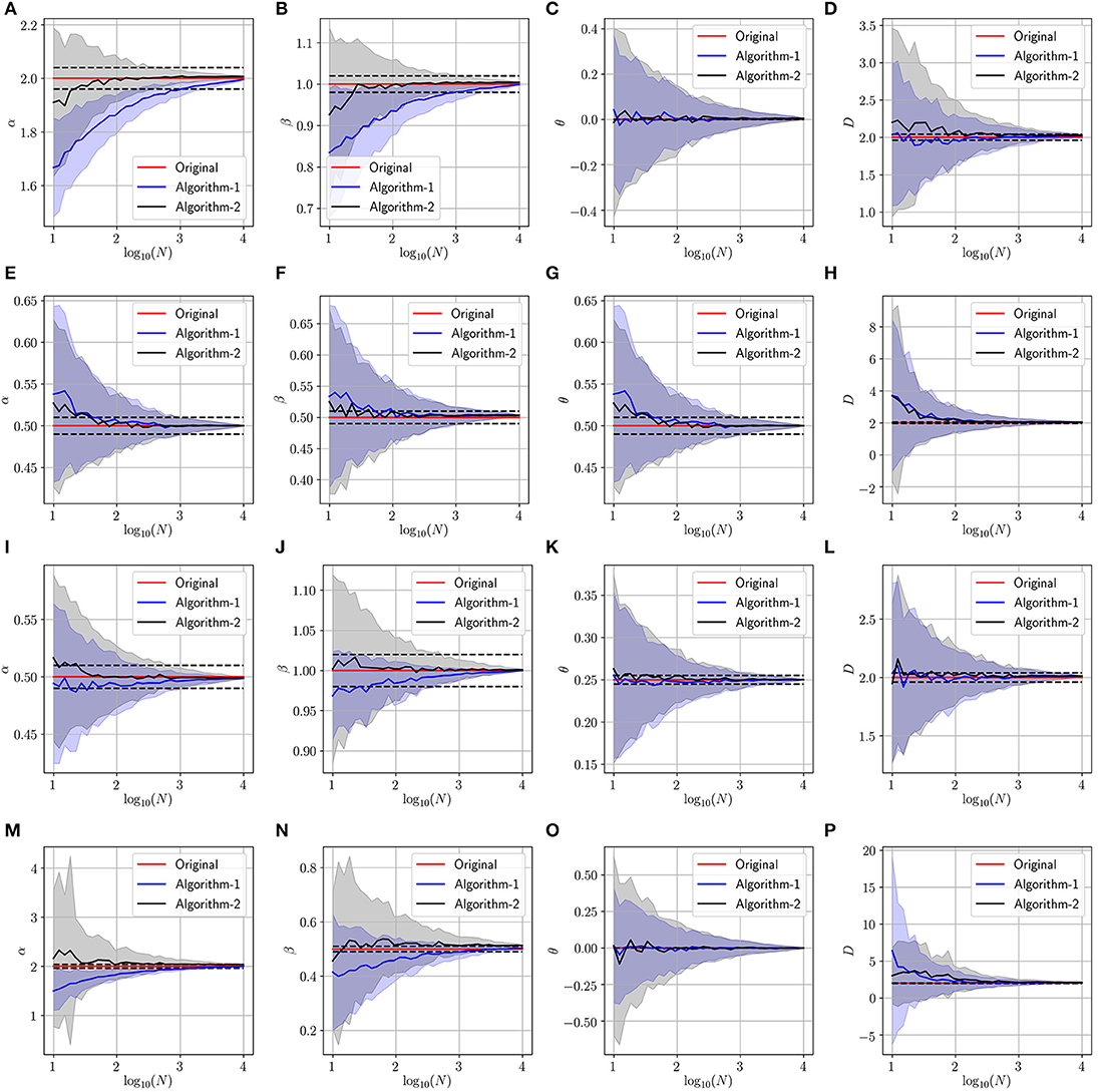
Figure 4. Determining the parameters of the space-time fractional diffusion via the two proposed algorithms while varying the number of trajectories and the generalized diffusion coefficient D = 2. The dotted line indicate 2% error tube around the original parameter value in the red: (A–D) Normal diffusion equation (α = 2, β = 1, θ = 0), (E–H) Neutral diffusion equation (α = 0.5, β = 0.5, θ = 0.5), (I–L) Space fractional diffusion equation (α = 0.5, β = 1, θ = 0.25), (M–P) Time fractional diffusion equation (α = 2, β = 0.5, θ = 0).

FIGURE 5

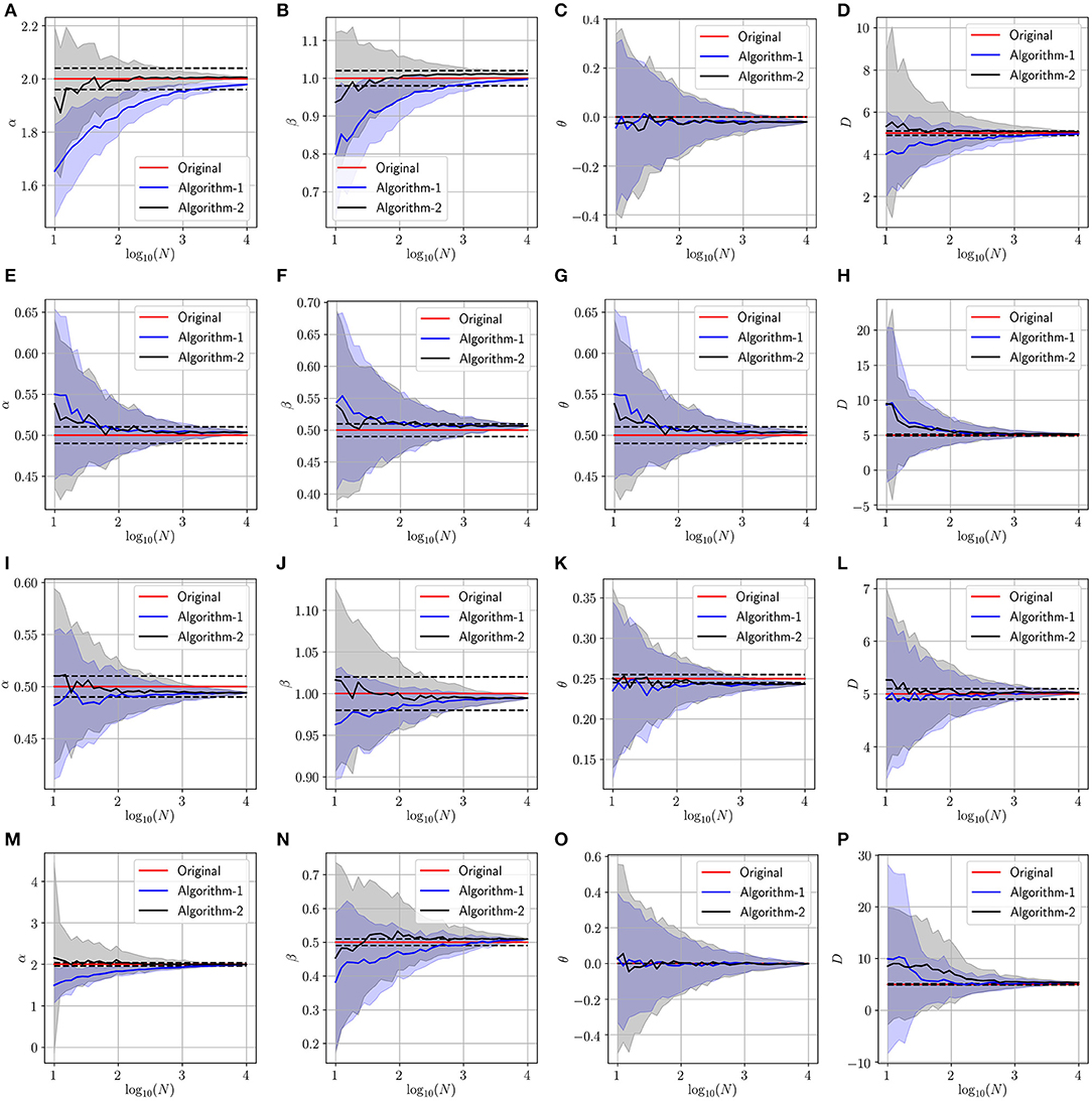
Figure 5. Determining the parameters of the space-time fractional diffusion via the two proposed algorithms while varying the number of trajectories and the generalized diffusion coefficient D = 5. The dotted line indicate 2% error tube around the original parameter value in the red: (A–D) Normal diffusion equation (α = 2, β = 1, θ = 0), (E–H) Neutral diffusion equation (α = 0.5, β = 0.5, θ = 0.5), (I–L) Space fractional diffusion equation (α = 0.5, β = 1, θ = 0.25), (M–P) Time fractional diffusion equation (α = 2, β = 0.5, θ = 0).

In Tables 1–3, we provide further details about the results we have described in Figures 3–5, respectively. Indeed, for both algorithms, we report the estimated value of each parameter, in the column entitled the final value, of the space-time fractional diffusion equation (i.e., α, β, θ and D) and the final relative error, which is defined as the percentage of the discrepancy between the exact value and the estimated one, or ${\epsilon }_{\xi }=\frac{|\widehat{\xi }-\xi |}{\left|\xi \right|}\times 100$, where $\widehat{\xi }$ and ξ are any estimated and original parameters, respectively. We also report the parameter $N_{90}^{(i)}$, which we define as the minimum number of trajectories beyond which the accuracy using algorithm i is at least 90% and formally can be written as

$\begin{array}{l}{N}_{90}^{(i)}(\xi )=inf\{N|{\epsilon }_{\xi }\le 10,\forall N>N_{90},\xi \leftarrow {{A}}_i({\{X_n(t_l)\}}_{n=1}^N)\},\end{array}$

where ξ ∈ {α, β, θ, D} and ${{A}}_i({\{X_n(t_l)\}}_{n=1}^N)$ denotes the output of the i-th Algorithm (i ∈ {1, 2}). By looking at the values reported in the column $N_{90}^{(i)}$, we can analyze the performance of both algorithms. For instance, we can remark that a dozen of trajectories is sufficient for both algorithms to achieve at least 90% accuracy in most of the settings. We note that a missing value for $N_{90}^{(i)}$ could be an indicator of either a bias in the Algorithm i which is greater than 10%, or the situation that the maximum considered trajectories (N = 10⁴) in our experiments are not sufficient enough for achieving accuracy more than 90%. Lastly, it is worth to note that increasing the number of trajectories will lead to a smaller final relative error.

TABLE 1

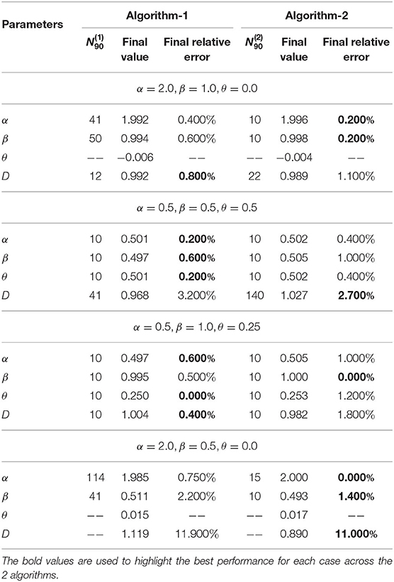
Table 1. Numerical results for fractional diffusion parameter estimation with D = 1.

TABLE 2

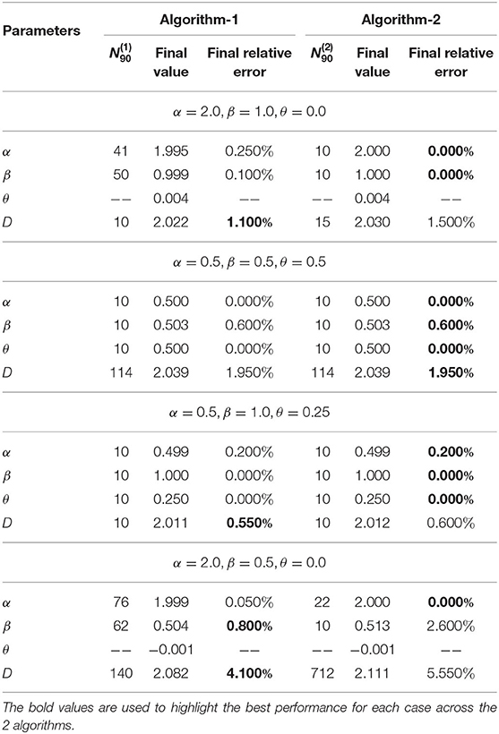
Table 2. Numerical results for fractional diffusion parameter estimation with D = 2.

TABLE 3

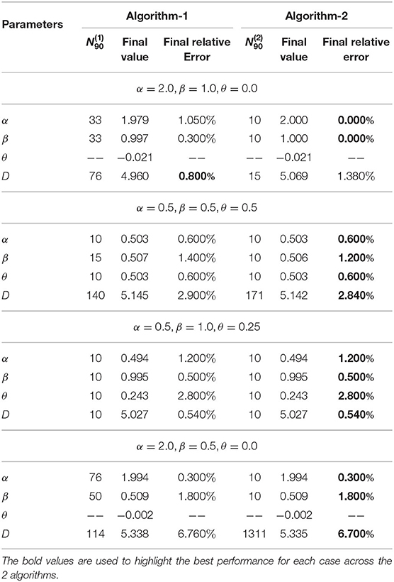
Table 3. Numerical results for fractional diffusion parameter estimation with D = 5.

3.2. Parameters Estimation of Fractional Brownian Motion

In this experiment, we present a study of fractional Brownian motion (fBm) process. More precisely, we consider a dataset of trajectories generated using the fBm model, then we parameterize the data according to the fractional diffusion equation under study in order to estimate the parameters of the fBm process generating the data (i.e., the Hurst exponent H and the diffusion constant D₀). From the Langevin equation associated with the fBm, we can remark that the fBm exhibits a long-time correlation which makes the process non-Markovian. The effective Fokker-Planck equation is given as

$\begin{array}{ll}\frac{\partial p(x,t)}{\partial t}=D_{0}2H{t}^{2H-1}\frac{{\partial }^{2}p(x,t)}{\partial x^2}.& (13)\end{array}$

The solution for the aforementioned equation is provided in Wang and Lung [72]

$\begin{array}{ll}p(x,t)=\frac{1}{\sqrt{4\pi D_0{t}^{2H}}}exp\left(\frac{-x^2}{4D_0{t}^{2H}}\right).& (14)\end{array}$

Thus, the fractional absolute moment of a fBm process with a parameter 0 < H < 0.5 is given as

$\begin{array}{ll}𝔼[|X(t){|}^{\delta }]={(2D_0{t}^{2H})}^{\delta /2}\frac{\Gamma (\frac{1+\delta }{2})}{\sqrt{\pi }}.& (15)\end{array}$

Based on the expressions (3) and (15), we can use the space-time fractional diffusion equation under study to parameterize an fBm process. Indeed, by mapping the two expressions, we get α = 2, β = 2H, θ = 0 and $D=\frac{D_0}{2}$. In this experiment, we assume that the given trajectories are following an fBm model and the task is to apply the proposed algorithms to identify the parameters associated with the fBm (H and D₀).

Last, in Figure 6, we present the simulation results associated with this experiment. The figure represents a panel of 4 × 4 plots where a row is associated with a set of parameters H and D₀ associated to a fBm process, and columns 1, 2, 3 and 4 are associated with the estimation of the parameters α, β, θ and D, respectively. Hence the estimation of the parameters H and D₀. In these simulations, we generate N trajectories following four different fBm models using the built-in function wfbm in Matlab (i.e., in Figure 6, rows 1, 2, 3 and 4 are associated to fBm with Hurst exponents H = 0.25, H = 0.3, H = 0.35 and H = 0.4, respectively). As we can observe, Algorithm 2 (plotted using black line) can efficiently provide accurate estimates of the Hurst exponent and the diffusion constant and it performs better than Algorithm 1. The reason behind this is that Algorithm 1 requires solving a non-linear non-convex optimization problem which is not the case for the second algorithm. Also, we remark that finding the parameters of the fBm using Algorithm 2 does not require very large number of trajectories. In fact, we can determine an accurate estimates of the parameters (α, β) with an error close to 2% by performing Algorithm 2 on dataset of few trajectories obeying the fBm model (i.e., N ≤ 10).

FIGURE 6

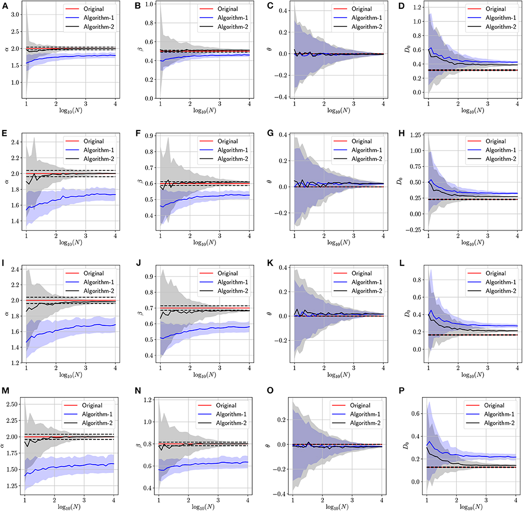
Figure 6. Determining the parameters of the fractional Brownian motion via the two proposed algorithms while varying the number of trajectories. The dotted line indicate 2% error tube around the original parameter value in the red: (A–D) with H = 0.25 and (α = 2, β = 2H, θ = 0, D₀ = 0.31), (E–H) with H = 0.3 and (α = 2, β = 2H, θ = 0, D₀ = 0.22), (I–L) with H = 0.35 and (α = 2, β = 2H, θ = 0, D₀ = 0.16), (M–P) with H = 0.4 and (α = 2, β = 2H, θ = 0, D₀ = 0.12).

From the simulation results related to fBm in Figure 6, we can see that Algorithm 2 is capable to accurately estimate the parameters α and β = 2H hence H. However, the estimation of the parameter D₀ is not accurate because of the non-conformity of the equation under study with the fBm model for all parameters values. Indeed, both models coincide, in terms of moments, only when α = 2, θ = 0 and β = 2H. Interestingly, in the current experiment, we focus more on determining an accurate estimate of the parameter H that is related to the long-time memory of an fBm process. Therefore, the proposed algorithms can be used as a tool to quantify the memory of an unknown process that follows the fBm model from given trajectories.

In Table 4, we report further elaboration of the results in Figure 6. In fact, we can remark that all the bold marked minimum relative errors are in the column associated with Algorithm 2, which endorse our previous claim about the effectiveness of the second algorithm. Related to the discussion of the estimation of α and β, we can see that the column $N_{90}^{(1)}$ has a lot of missing values, and this indicates that using Algorithm 1 for these experiments lead to a final relative error that is greater than 10%. More interestingly, we can remark that with just around 10 trajectories, Algorithm 2 can provide an estimate of either α or β that is within the 10% error margin.

TABLE 4

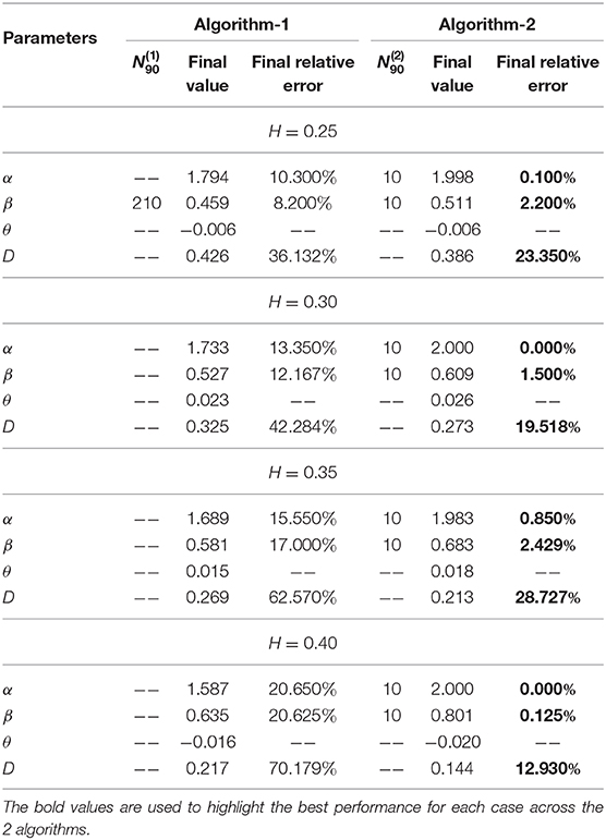
Table 4. Numerical results for fBm parameter estimation.

4. Discussion

Understanding complex dynamics remains a challenging task when their generative model is unknown. This task is more complicated when it comes to analyze spatiotemporal kinetics and infer the model that dictate their evolution. Although, the physics that drive the dynamics are unknowns, data-driven based approaches are prominent tools to discover the physical laws/rules governing complex observed dynamics (from heterogeneous, sparse, scarce or even noisy data). Indeed, such a discovery plays a crucial role in diverse fields ranging from system biology, neuroscience, econophysics to social studies. Toward addressing this goal, in this manuscript, we have considered a generalized space-time fractional PDE and have developed an effective, rigorous and robust algorithmic strategies to estimate the parameters and so identify the main mathematical operators appearing in the PDE.

In contrast to prior work, we investigated the effectiveness and robustness of the proposed algorithmic approach for estimating the correct parameters as a function of the available number of trajectories. From our simulation results, we observe that for all considered types of diffusion models except the classical one (i.e., all combination of the parameters α, β, θ, and D), a few number of recorded time-series (less than 100 trajectories) is required to attain the correct estimation of the PDE parameters with less then 2% confidence interval. For the case of the normal diffusion (i.e., except for the case α = 2 and β = 1), we may need more trajectories to achieve similar accuracy. Therefore, we hope that the proposed algorithms will help the community to better analyze complex spatiotemporal data, in order to unravel new physical laws in different applications (social networks, neuroscience, etc.) and decipher the causal interdependence between different processes.

Furthermore, we performed a study on the properties of fBm processes. We can remark from the Fokker Planck equation associated with the fBm process, mentioned in the manuscript, that the effective diffusion coefficient is time-dependent. Even though, this type of equation does not perfectly match the class of fractional diffusion equation that we are dealing with in this work, we applied the proposed algorithms to a dataset of trajectories generated according to the fBm model to retrieve the Hurst exponent and the diffusion constant. Indeed, we were able to identify these parameters since the absolute and signed absolute moments present similar structure as the ones calculated for a process that is generated according to the fractional diffusion equation under study. Therefore, we provide a new/alternative approach to quantify the memory of a fBm process. Note that without knowing the model that governs the dynamics of the process and using this framework, we can estimate the parameters α and θ to be equal to 2 and 0, respectively, but in the current stage we are not able to confirm that the data is generated either from a space-time fractional diffusion equation with a constant generalized diffusion coefficient or from a fBm process with time varying diffusion coefficient. In future work, we will push forward the analysis to identify whether the diffusion coefficient is time-dependent or it is a constant, and thus to differentiate between the space-time fractional diffusion equation and the Fokker Planck equation associated with the fBm process.

This mathematical formalism can be further developed and generalized to include additional operators and take into account advection phenomena as well as combined with other advanced statistics and information theory inspired methods to discriminate among various mathematical expressions (operators) in order to either identify the dominant physical phenomenon (or rule) governing the measurements or to determine the degree to which multiple physical laws contribute to the observed dynamics. Also, analyzing noisy data originated from real world applications will be taken into account in order to cope with complex scenario. We plan to build on these grounds, enrich the mathematical formalism and contribute to a significant paradigm shift in the context of data-driven discovery architectures of physical phenomena as well as enabling accurate predictions concerning complex evolving systems without requiring to know the regimes of variation for parameters, the types of mathematical operators or the fact that the data should be sampled at a particular level.

Data Availability Statement

The raw data supporting the conclusions of this article will be made available by the authors, without undue reservation, to any qualified researcher.

Author Contributions

MZ and GG have equal contribution to the manuscript. MZ, GG, and PB contributed to formulating the problem, setup the experimental case studies, and wrote the manuscript. MZ and GG collaborated on the design of the simulations, run comprehensive case studies, processed the simulation data, prepared the plots and modified the supplementary material. KA contributed to the design of some of the simulations and wrote some parts of the supplementary material.

Funding

The authors gratefully acknowledge the support by the National Science Foundation under the Career Award CPS/CNS-1453860, the NSF award under Grant numbers CCF-1837131, MCB-1936775, and CNS-1932620, the U.S. Army Research Office (ARO) under Grant No. W911NF-17-1-0076 and the DARPA Young Faculty Award and DARPA Director Award, under grant number N66001-17-1-4044, and a Northrop Grumman grant. The views, opinions, and/or findings contained in this article are those of the authors and should not be interpreted as representing the official views or policies, either expressed or implied by the Defense Advanced Research Projects Agency, the Department of Defense or the National Science Foundation.

Conflict of Interest

The authors declare that the research was conducted in the absence of any commercial or financial relationships that could be construed as a potential conflict of interest.

Supplementary Material

The Supplementary Material for this article can be found online at: https://www.frontiersin.org/articles/10.3389/fams.2020.00014/full#supplementary-material

The code to reproduce the results is available at: https://github.com/gaurav71531/fractDiffusion.

Footnotes

1. ^The two operators are clearly defined in the Supplementary Material.

2. ^Additional simulations for other scenarios are presented in the Supplementary Material.

References

1. Alber M, Tepole AB, Cannon WR, De S, Dura-Bernal S, Garikipati K, et al. Integrating machine learning and multiscale modeling–perspectives, challenges, and opportunities in the biological, biomedical, and behavioral sciences. NPJ Digital Med. (2019) 2:115. doi: 10.1038/s41746-019-0193-y

PubMed Abstract | CrossRef Full Text | Google Scholar

2. Gruson D, Helleputte T, Rousseau P, Gruson D. Data science, artificial intelligence, and machine learning: Opportunities for laboratory medicine and the value of positive regulation. Clin Biochem. (2019) 69:1–7. doi: 10.1016/j.clinbiochem.2019.04.013

PubMed Abstract | CrossRef Full Text | Google Scholar

3. Bergen KJ, Johnson PA, de Hoop MV, Beroza GC. Machine learning for data-driven discovery in solid Earth geoscience. Science. (2019) 363:eaau0323. doi: 10.1126/science.aau0323

PubMed Abstract | CrossRef Full Text | Google Scholar

4. He J, Baxter SL, Xu J, Xu J, Zhou X, Zhang K. The practical implementation of artificial intelligence technologies in medicine. Nat Med. (2019) 25:30–36. doi: 10.1038/s41591-018-0307-0

PubMed Abstract | CrossRef Full Text | Google Scholar

5. Barnette DA, Davis MA, Dang NL, Pidugu AS, Hughes T, Swamidass SJ, et al. Lamisil (terbinafine) toxicity: determining pathways to bioactivation through computational and experimental approaches. Biochem Pharmacol. (2018) 156:10–21. doi: 10.1016/j.bcp.2018.07.043

PubMed Abstract | CrossRef Full Text | Google Scholar

6. Udrescu L, Sbarcea L, Topirceanu A, Iovanovici A, Kurunczi L, Bogdan P, et al. Clustering drug-drug interaction networks with energy model layouts: community analysis and drug repurposing. Sci Rep. (2016) 6:32745. doi: 10.1038/srep32745

PubMed Abstract | CrossRef Full Text | Google Scholar

7. Marinelli B, Kang M, Martini M, Zech JR, Titano J, Cho S, et al. Combination of active transfer learning and natural language processing to improve liver volumetry using surrogate metrics with deep learning. Radiol Artif Intell. (2019) 1:e180019. doi: 10.1148/ryai.2019180019

CrossRef Full Text | Google Scholar

8. Yang J, Feng X, Laine A, Angelini E. Characterizing Alzheimer's disease with image and genetic biomarkers using supervised topic models. IEEE J Biomed Health Inform. (2019) 24:1180–7. doi: 10.1109/JBHI.2019.2928831

PubMed Abstract | CrossRef Full Text | Google Scholar

9. Hazlett HC, Gu H, Munsell BC, Kim SH, Styner M, Wolff JJ, et al. Early brain development in infants at high risk for autism spectrum disorder. Nature. (2017) 542:348. doi: 10.1038/nature21369

PubMed Abstract | CrossRef Full Text | Google Scholar

10. Ting DSW, Pasquale LR, Peng L, Campbell JP, Lee AY, Raman R, et al. Artificial intelligence and deep learning in ophthalmology. Brit J Ophthalmol. (2019) 103:167–75. doi: 10.1136/bjophthalmol-2018-313173

PubMed Abstract | CrossRef Full Text | Google Scholar

11. Furquim G, Pessin G, Faiçal BS, Mendiondo EM, Ueyama J. Improving the accuracy of a flood forecasting model by means of machine learning and chaos theory. Neural Comput Appl. (2016) 27:1129–41. doi: 10.1007/s00521-015-1930-z

CrossRef Full Text | Google Scholar

12. Mojaddadi H, Pradhan B, Nampak H, Ahmad N, bin Ghazali AH. Ensemble machine-learning-based geospatial approach for flood risk assessment using multi-sensor remote-sensing data and GIS. Geomat Nat Hazards Risk. (2017) 8:1080–102. doi: 10.1080/19475705.2017.1294113

CrossRef Full Text | Google Scholar

13. Fox C, Nicholls G. Statistical estimation of the parameters of a PDE. Can appl Math Quater. (2001) 10:277–306.

Google Scholar

14. Müller TG, Timmer J. Fitting parameters in partial differential equations from partially observed noisy data. Phys D Nonlinear Phenomena. (2002) 171:1–7. doi: 10.1016/S0167-2789(02)00546-8

CrossRef Full Text | Google Scholar

15. Xun X, Cao J, Mallick B, Maity A, Carroll RJ. Parameter estimation of partial differential equation models. J Am Stat Assoc. (2013) 108:1009–20. doi: 10.1080/01621459.2013.794730

PubMed Abstract | CrossRef Full Text | Google Scholar

16. Liang H, Wu H. Parameter estimation for differential equation models using a framework of measurement error in regression models. J Am Stat Assoc. (2008) 103:1570–83. doi: 10.1198/016214508000000797

PubMed Abstract | CrossRef Full Text | Google Scholar

17. Bär M, Hegger R, Kantz H. Fitting partial differential equations to space-time dynamics. Phys Rev E. (1999) 59:337. doi: 10.1103/PhysRevE.59.337

CrossRef Full Text | Google Scholar

18. Müller T, Timmer J. Parameter identification techniques for partial differential equations. Int J Bifurcat Chaos. (2004) 14:2053–60. doi: 10.1142/S0218127404010424

CrossRef Full Text | Google Scholar

19. Voss HU, Kolodner P, Abel M, Kurths J. Amplitude equations from spatiotemporal binary-fluid convection data. Phys Rev Lett. (1999) 83:3422. doi: 10.1103/PhysRevLett.83.3422

CrossRef Full Text | Google Scholar

20. Einstein A. Über die von der molekularkinetischen Theorie der Wärme geforderte Bewegung von in ruhenden Flüssigkeiten suspendierten Teilchen. Annalen der Physik. (1905). 322:549–60. doi: 10.1002/andp.19053220806

CrossRef Full Text | Google Scholar

21. Barkai E, Garini Y, Metzler R. Strange kinetics of single molecules in living cells. Phys Tdy. (2012) 65:29–5. doi: 10.1063/PT.3.1677

CrossRef Full Text | Google Scholar

22. Tolić-Nørrelykke IM, Munteanu EL, Thon G, Oddershede L, Berg-Sorensen K. Anomalous diffusion in living yeast cells. Phys Rev Lett. (2004) 93:078102. doi: 10.1103/PhysRevLett.93.078102

PubMed Abstract | CrossRef Full Text | Google Scholar

23. Jeon JH, Tejedor V, Burov S, Barkai E, Selhuber-Unkel C, Berg-Sørensen K, et al. In vivo anomalous diffusion and weak ergodicity breaking of lipid granules. Phys Rev Lett. (2011) 106:048103. doi: 10.1103/PhysRevLett.106.048103

PubMed Abstract | CrossRef Full Text | Google Scholar

24. Goychuk I. Anomalous transport of subdiffusing cargos by single kinesin motors: the role of mechano-chemical coupling and anharmonicity of tether. Phys Biol. (2015) 12:016013. doi: 10.1088/1478-3975/12/1/016013

PubMed Abstract | CrossRef Full Text | Google Scholar

25. Koorehdavoudi H, Bogdan P, Wei G, Marculescu R, Zhuang J, Carlsen RW, et al. Multi-fractal characterization of bacterial swimming dynamics: a case study on real and simulated serratia marcescens. Proc R Soc A Math Phys Eng Sci. (2017) 473:20170154. doi: 10.1098/rspa.2017.0154

PubMed Abstract | CrossRef Full Text | Google Scholar

26. Papo D. Functional significance of complex fluctuations in brain activity: from resting state to cognitive neuroscience. Front Syst Neurosci. (2014) 8:112. doi: 10.3389/fnsys.2014.00112

PubMed Abstract | CrossRef Full Text | Google Scholar

27. Gupta G, Pequito S, Bogdan P. Dealing with unknown unknowns: Identification and selection of minimal sensing for fractional dynamics with unknown inputs. In: 2018 Annual American Control Conference (ACC). Milwaukee, WI: IEEE (2018). p. 2814–20. doi: 10.23919/ACC.2018.8430866

CrossRef Full Text | Google Scholar

28. Gupta G, Pequito S, Bogdan P. Learning latent fractional dynamics with unknown unknowns. In: 2019 American Control Conference (ACC). Philadelphia, PA (2019). p. 217–22. doi: 10.23919/ACC.2019.8815074

CrossRef Full Text | Google Scholar

29. Xue Y, Bogdan P. Constructing compact causal mathematical models for complex dynamics. In: Proceedings of the 8th International Conference on Cyber-Physical Systems. ICCPS '17. Pittsburgh, PA: ACM (2017). p. 97–107. doi: 10.1145/3055004.3055017

CrossRef Full Text | Google Scholar

30. Yang R, Gupta G, Bogdan P. Data-driven perception of neuron point process with unknown unknowns. In: Proceedings of the 10th ACM/IEEE International Conference on Cyber-Physical Systems. ICCPS '19. Montreal, QC (2019). p. 259–69. doi: 10.1145/3302509.3311056

PubMed Abstract | CrossRef Full Text | Google Scholar

31. Gefen Y, Aharony A, Alexander S. Anomalous diffusion on percolating clusters. Phys Rev Lett. (1983) 50:77–80. doi: 10.1103/PhysRevLett.50.77

CrossRef Full Text | Google Scholar

32. Klafter J, Blumen A, Shlesinger MF. Stochastic pathway to anomalous diffusion. Phys Rev A. (1987) 35:3081–5. doi: 10.1103/PhysRevA.35.3081

PubMed Abstract | CrossRef Full Text | Google Scholar

33. Bouchaud JP, Georges A. Anomalous diffusion in disordered media: Statistical mechanisms, models and physical applications. Phys Rep. (1990) 195:127–293. doi: 10.1016/0370-1573(90)90099-N

CrossRef Full Text | Google Scholar

34. Metzler R, Klafter J. The random walk's guide to anomalous diffusion: a fractional dynamics approach. Phys Rep. (2000) 339:1–77. doi: 10.1016/S0370-1573(00)00070-3

CrossRef Full Text | Google Scholar

35. Metzler R, Glockle WG, Nonnenmacher TF. Fractional model equation for anomalous diffusion. Phys A Stat Mech Appl. (1994) 211:13–24. doi: 10.1016/0378-4371(94)90064-7

CrossRef Full Text | Google Scholar

36. Metzler R, Klafter J. The restaurant at the end of the random walk: recent developments in the description of anomalous transport by fractional dynamics. J Phys A Math Gen. (2004) 37:R161. doi: 10.1088/0305-4470/37/31/R01

CrossRef Full Text | Google Scholar

37. Klafter J, Sokolov IM. Anomalous diffusion spreads its wings. Phys World. (2005) 18:29–32. doi: 10.1088/2058-7058/18/8/33

CrossRef Full Text | Google Scholar

38. Thiel F, Flegel F, Sokolov IM. Disentangling sources of anomalous diffusion. Phys Rev Lett. (2013) 111:010601. doi: 10.1103/PhysRevLett.111.010601

PubMed Abstract | CrossRef Full Text | Google Scholar

39. McKinley SA, Nguyen HD. Anomalous diffusion and the generalized Langevin equation. SIAM J Math Anal. (2018) 50:5119–60. doi: 10.1137/17M115517X

CrossRef Full Text | Google Scholar

40. Oliveira FA, Ferreira RMS, Lapas LC, Vainstein MH. Anomalous diffusion: a basic mechanism for the evolution of inhomogeneous systems. Front Phys. (2019) 7:18. doi: 10.3389/fphy.2019.00018

CrossRef Full Text | Google Scholar

41. Morgado R, Oliveira FA, Batrouni GG, Hansen A. Relation between anomalous and normal diffusion in systems with memory. Phys Rev Lett. (2002) 89:100601. doi: 10.1103/PhysRevLett.89.100601

PubMed Abstract | CrossRef Full Text | Google Scholar

42. Metzler R, Jeon JH, Cherstvy AG, Barkai E. Anomalous diffusion models and their properties: non-stationarity, non-ergodicity, and ageing at the centenary of single particle tracking. Phys Chem Chem Phys. (2014) 16:24128–64. doi: 10.1039/C4CP03465A

PubMed Abstract | CrossRef Full Text | Google Scholar

43. Sokolov IM. Models of anomalous diffusion in crowded environments. Soft Matter. (2012) 8:9043–52. doi: 10.1039/c2sm25701g

CrossRef Full Text | Google Scholar

44. Grmela M, Öttinger HC. Dynamics and thermodynamics of complex fluids. I. Development of a general formalism. Phys Rev E. (1997) 56:6620. doi: 10.1103/PhysRevE.56.6620

CrossRef Full Text | Google Scholar

45. Cabreira RG, da Silva Ferreira A, Kouyaté M, Demouchy G, Mériguet G, Aquino R, et al. Thermodiffusion of repulsive charged nanoparticles-the interplay between single-particle and thermoelectric contributions. Phys Chem Chem Phys. (2018) 20:16402–13. doi: 10.1039/C8CP02558D

PubMed Abstract | CrossRef Full Text | Google Scholar

46. Brangwynne CP, Koenderink GH, MacKintosh FC, Weitz DA. Intracellular transport by active diffusion. Trends Cell Biol. (2009) 19:423–7. doi: 10.1016/j.tcb.2009.04.004

PubMed Abstract | CrossRef Full Text | Google Scholar

47. Palmieri B, Bresler Y, Wirtz D, Grant M. Multiple scale model for cell migration in monolayers: elastic mismatch between cells enhances motility. Sci Rep. (2015) 5:11745. doi: 10.1038/srep11745

PubMed Abstract | CrossRef Full Text | Google Scholar

48. Lomholt MA, Ambjörnsson T, Metzler R. Optimal target search on a fast-folding polymer chain with volume exchange. Phys Rev Lett. (2005) 95:260603. doi: 10.1103/PhysRevLett.95.260603

PubMed Abstract | CrossRef Full Text | Google Scholar

49. Klages R, Radons G, Sokolov IM. Anomalous Transport: Foundations and Applications. Weinheim: John Wiley & Sons, Ltd. (2008). doi: 10.1002/9783527622979

CrossRef Full Text | Google Scholar

50. Mandelbrot BB. The Fractal Geometry of Nature. Einaudi Paperbacks. 3rd edn. San Francisco, CA: W. H. Freeman and Company (1983). Available online at: https://books.google.com/books?id=SWcPAQAAMAAJ

Google Scholar

51. Balankin AS. Mapping physical problems on fractals onto boundary value problems within continuum framework. Phys Lett A. (2018) 382:141–46. doi: 10.1016/j.physleta.2017.11.005

CrossRef Full Text | Google Scholar

52. Bogdan P, Marculescu R. A fractional calculus approach to modeling fractal dynamic games. In: 2011 50th IEEE Conference on Decision and Control and European Control Conference. Orlando, FL: IEEE (2011). p. 255–60. doi: 10.1109/CDC.2011.6161323

CrossRef Full Text | Google Scholar

53. Scalas E. The application of continuous-time random walks in finance and economics. Phys A Stat Mech Appl. (2006) 362:225–39. doi: 10.1016/j.physa.2005.11.024

CrossRef Full Text | Google Scholar

54. Morgado R, Cieśla M, Longa L, Oliveira FA. Synchronization in the presence of memory. Europhys Lett. (2007) 79:10002. doi: 10.1209/0295-5075/79/10002

CrossRef Full Text | Google Scholar

55. Lapas L, Costa I, Vainstein M, Oliveira F. Entropy, non-ergodicity and non-Gaussian behaviour in ballistic transport. Europhys Lett. (2007) 77:37004. doi: 10.1209/0295-5075/77/37004

CrossRef Full Text | Google Scholar

56. Kusmierz L, Dybiec B, Gudowska-Nowak E. Thermodynamics of superdiffusion generated by Lévy-Wiener fluctuating forces. Entropy. (2018) 20:658. doi: 10.3390/e20090658

CrossRef Full Text | Google Scholar

57. Pérez-Madrid A. Gibbs entropy and irreversibility. Phys A Stat Mech Appl. (2004) 339:339–46. doi: 10.1016/j.physa.2004.04.106

CrossRef Full Text | Google Scholar

58. Gorenflo R, Mainardi F. Fractional diffusion processes: probability distributions and continuous time random walk. In: Rangarajan G, Ding M, editors. Processes with Long-Range Correlations: Theory and Applications. Berlin; Heidelberg: Springer (2003). p. 148–66. doi: 10.1007/3-540-44832-2_8

CrossRef Full Text | Google Scholar

59. Metzler R, Barkai E, Klafter J. Anomalous diffusion and relaxation close to thermal equilibrium: a fractional Fokker-Planck equation approach. Phys Rev Lett. (1999) 82:3563–7. doi: 10.1103/PhysRevLett.82.3563

CrossRef Full Text | Google Scholar

60. Schwarzl M, Godec A, Metzler R. Quantifying non-ergodicity of anomalous diffusion with higher order moments. Sci Rep. (2017) 7:3878. doi: 10.1038/s41598-017-03712-x

PubMed Abstract | CrossRef Full Text | Google Scholar

61. Gorenflo R, Mainardi F. Parametric subordination in fractional diffusion processes. arXiv preprint arXiv:12108414 (2012). doi: 10.1142/9789814340595_0010

CrossRef Full Text | Google Scholar

62. Mainardi F, Luchko Y, Pagnini G. The fundamental solution of the space-time fractional diffusion equation. arXiv preprint arXiv:cond-mat/0702419 (2007).

Google Scholar

63. Saichev AI, Zaslavsky GM. Fractional kinetic equations: solutions and applications. Chaos. (1997) 7:753–64. doi: 10.1063/1.166272

PubMed Abstract | CrossRef Full Text | Google Scholar

64. Gorenflo R, Iskenderov A, Luchko Y. Mapping between solutions of fractional diffusion-wave equations. Fract Calculus Appl Anal. (2000) 3:75–86.

Google Scholar

65. Scalas E, Gorenflo R, Mainardi F. Fractional calculus and continuous-time finance. Phys A Stat Mech Appl. (2000) 284:376–84. doi: 10.1016/S0378-4371(00)00255-7

CrossRef Full Text | Google Scholar

66. Feller W. On a Generalization of Marcel Riesz' Potentials and the Semi-groups Generated by Them. Gleerup. (1962) Available online at: https://books.google.com/books?id=UZTqjwEACAAJ

Google Scholar

67. Caputo M. Linear models of dissipation whose Q is almost frequency independent-II. Geophys J Int. (1967) 13:529–39. doi: 10.1111/j.1365-246X.1967.tb02303.x

CrossRef Full Text | Google Scholar

68. Gorenflo R, Mainardi F, Moretti D, Pagnini G, Paradisi P. Discrete random walk models for space-time fractional diffusion. Chem Phys. (2002) 284:521–41. doi: 10.1016/S0301-0104(02)00714-0

CrossRef Full Text | Google Scholar

69. Metzler R, Nonnenmacher TF. Space- and time-fractional diffusion and wave equations, fractional Fokke-Planck equations, and physical motivation. Chem Phys. (2002) 284:67–90. doi: 10.1016/S0301-0104(02)00537-2

CrossRef Full Text | Google Scholar

70. Luchko Y. Models of the neutral-fractional anomalous diffusion and their analysis. AIP Conf Proc. (2012) 1493:626–32. doi: 10.1063/1.4765552

CrossRef Full Text | Google Scholar

71. Tarasov VE. Handbook of Fractional Calculus with Applications: Applications in Physics (Part 2). Berlin; Boston, MA: De Gruyter (2019).

Google Scholar

72. Wang K, Lung C. Long-time correlation effects and fractal Brownian motion. Phys Lett A. (1990) 151:119–21. doi: 10.1016/0375-9601(90)90175-N

CrossRef Full Text | Google Scholar