Prony-Type Polynomials and Their Common Zeros

The problem of hidden periodicity of a bivariate exponential sum $f(\text{n})={\sum }_{j=1}^N{a}_{j}exp(-\text{i}\langle {\omega }_j,\text{n}\rangle ),$ where a₁, …, a_N ∈ ℂ\{0} and n ∈ ℤ², is to recover frequency vectors ${\omega }_1,\dots ,{\omega }_N\in [0,2\pi ){}^2$ using finitely many samples of f. Recently, this problem has received a lot of attention, and different approaches have been proposed to obtain its solution. For example, Kunis et al. [1] relies on the kernel basis analysis of the multilevel Toeplitz matrix of moments of f. In Cuyt et al. [2], the exponential analysis has been considered as a Padé approximation problem. In contrast to the previous method, the algorithms developed in Diederichs and Iske [3] and Cuyt and Wen-Shin [4] use sampling of f along several lines in the hyperplane to obtain the univariate analog of the problem, which can be solved by classical one-dimensional approaches. Nevertheless, the stability of numerical solutions in the case of noise corruption still has a lot of open questions, especially when the number of parameters increases. Inspired by the one-dimensional approach developed in Filbir et al. [5], we propose to use the method of Prony-type polynomials, where the elements ω₁, …, ω_N can be recovered due to a set of common zeros of the monic bivariate polynomial of an appropriate multi-degree. The use of Cantor pairing functions allows us to express bivariate Prony-type polynomials in terms of determinants and to find their exact algebraic representation. With respect to the number of samples the method of Prony-type polynomials is situated between the methods proposed in Kunis et al. [1] and Cuyt and Wen-Shin [4]. Although the method of Prony-type polynomials requires more samples than Cuyt and Wen-Shin [4], numerical computations show that the algorithm behaves more stable with regard to noisy data. Besides, combining the method of Prony-type polynomials with an autocorrelation sequence allows the improvement of the stability of the method in general.

1. Introduction

Let N ∈ ℕ be an integer, a₁, a₂, …, a_N ∈ ℂ\{0} and ${\omega }_j=({\omega }_{j,1},{\omega }_{j,2})\in [0,2\pi ){}^2$ with ω_j ≠ ω_k for j ≠ k, j, k = 1, …, N. Let us consider a function f : ℤ² → ℂ of the form

$\begin{array}{ll}f(\text{n})={\displaystyle \sum _{j=1}^N}{a}_{j}exp(-\text{i}\langle {\omega }_j,\text{n}\rangle ),& (1)\end{array}$

where $\text{n}=(n_1,n_2)\in {\mathbb{Z}}^2=\mathbb{Z}\times \mathbb{Z}$ and 〈ω_j, n〉 = ω_j,1n₁ + ω_j,2n₂. The function f is called N-sparse bivariate exponential sum with the pairwise distinct frequency vectors ω₁, ω₂, …, ω_N and coefficients a₁, a₂, …, a_N.

The problem of hidden periodicities (the PHP problem) is to find vectors ω₁, ω₂, …, ω_N out of finitely many function evaluations $f(\text{n}),\text{n}\in {N}\subset {\mathbb{Z}}_{+}^2,\#{N}<\infty$, that are called samples of f. The PHP problem is a fundamental problem in digital signal processing and has many practical applications [6–8]. Besides, similar problems occur in other fields of mathematical analysis (see, for example, [9]).

It is convenient to use the following notations for the exponent vectors

$\begin{array}{r}exp(-\text{i}{\omega }_j)=(exp(-\text{i}{\omega }_{j,1}),exp(-\text{i}{\omega }_{j,2}))=(z_{j,1},z_{j,2})={\text{z}}_j,\\ j=1,\dots ,N,\end{array}$

that together with the multi-index notation ${\text{z}}_j^{\text{n}}=z_{j,1}^{n_1}{z}_{j,2}^{n_2}$ for $\text{n}=(n_1,n_2)\in {\mathbb{Z}}^2$ allows us to rewrite the exponential sum (1) in a litte bit more compact form

$\begin{array}{ll}f(\text{n})={\displaystyle \sum _{j=1}^N}{a}_j{\text{z}}_j^{\text{n}}.& (2)\end{array}$

In the representation (2), the elements ${\text{z}}_1,\dots ,{\text{z}}_N\subset {𝕋}^2=𝕋\times 𝕋$, where 𝕋 = {z ∈ ℂ : |z| = 1} stands for the torus, are called the parameters of the exponential sum f. In such a way, instead of dealing with detecting the frequency vectors ω₁, ω₂, …, ω_N, one can consider an analogous problem and search for the parameters z₁, …, z_N. The problem of finding the parameters z₁, …, z_N using finitely many samples f is called the problem of parameter estimation of an exponential sum f.

The univariate problem of the parameter estimation has been considered initially by de Prony [10]. For a one-dimensional exponential sum

$\begin{array}{l}f(n)={\displaystyle \sum _{j=1}^N}{a}_{j}exp(-\text{i}{\omega }_{j}n)={\displaystyle \sum _{j=1}^N}{a}_j{z}_j^n,n\in \mathbb{Z},\end{array}$

Prony has proposed to recover the unknown parameters by computing the simple roots of the so-called Prony polynomial

$\begin{array}{ll}p(z)={\displaystyle \prod _{j=1}^N}(z-z_j)={\displaystyle \sum _{k=0}^N}{p}_k{z}^k& (3)\end{array}$

with the leading term p_N = 1 and with the following properties of the coefficients

$\begin{array}{l}{\displaystyle \sum _{k=0}^N}{p}_{k}f(k-q)={\displaystyle \sum _{j=1}^N}{a}_j{z}_j^{-q}{\displaystyle \sum _{k=0}^N}{p}_k{z}_j^k={\displaystyle \sum _{j=1}^N}{a}_j{z}_j^{-q}p(z_j)=0,\\ q=0,\dots ,N-1.& (4)\end{array}$

Given the samples f(n) for n = −N + 1, …, N, one can find the coefficients of the Prony polynomial by solving the linear system of Equations (4). The obtained system can be written in matrix form as

$\begin{array}{ll}{T}_N\text{p}=-{\text{f}}_N,& (5)\end{array}$

where $T_N(f)={(f_{i-j})}_{i,j=0}^{N-1}\in {ℂ}^{N\times N}$ is the Toeplitz matrix, $\text{p}={(p_0,p_1,\dots ,p_{N-1})}^{\text{T}}\in {ℂ}^N$ is the vector of polynomial coefficients and ${\text{f}}_N=(f_N,f_{N-1},\dots ,f_1{)}^{\text{T}}\in {ℂ}^N$ is a column vector of some additional samples of f with f(n) = f_n for all n ∈ ℤ. Analogically one can write the Prony polynomial in the determinant form as

After specifying the Prony polynomial, it is easy to detect the required parameters and consequently find the frequencies ω₁, ω₂, …, ω_N. The advantage of Prony's method is its simplicity. However, such method is unstable in the case of noisy data, i.e., when

$f(n)={\displaystyle \sum _{j=1}^N}{a}_{j}exp(-\text{i}{\omega }_{j}n)+\epsilon (n),n\in \mathbb{N},$

with a noisy part ε(n) of the signal.

Recently, the problem of parameter estimation, in general, and Prony's method, in particular, have received a lot of attention, and different approaches have been proposed to obtain a solution. On the one hand, various approaches have been developed to stabilize Prony's method (see [5, 11, 12]). For example, in Filbir et al. [5] the use of orthogonal polynomials and an autocorrelation sequence enabled stability. Newly, in Cuyt et al. [2], the exponential analysis has been considered as a Padé approximation problem which has helped to restore the parameters even though the separation distance between them is small. On the other hand, the question about the generalization of Prony's method to the multidimensional case has been raised [13, 14]. Among the multivariate techniques, the first complete generalization has been proposed in Kunis et al. [1]. This method relies on the kernel basis analysis of the multilevel Toeplitz matrix of moments of f, and requires at least (2N + 1)^d samples, where d denotes the dimension. In contrast to the previous one, the algorithms developed in Potts and Tasche [15], Diederichs and Iske [3], and Cuyt and Wen-Shin [4] use sampling of f along several lines in the hyperplane to obtain the univariate analog of the problem, which can be solved by classical one-dimensional approaches. Let us remark that the method proposed by Cuyt and Wen-Shin [4] is characterized by the absolute minimum of samples (d + 1)N, where d again is the dimension of the problem. The same problem has been considered in Sauer [16] on the hyperbolic cross, where it was shown that the Prony's problem with N frequency vectors can be solved using at most (d + 1)N²log^{2d − 2}N evaluations of f. Very recently, for a real coefficient set a₁, a₂, …, a_N ∈ ℝ\{0}, the multidimensional problem of parameter estimation has been considered as a type of sparse polynomial interpolation problem Nevertheless, for the complex setting the stability of numerical solutions in the case of noisy data still has a lot of open questions, especially when the number of parameters increases.

Motivated by Pan and Saff [18] and Filbir et al. [5], we propose the method of Prony-type polynomials in the two-dimensional case, where the parameters z₁, …, z_N can be recovered as a set of common zeros of the monic bivariate polynomial of an appropriate multi-degree. Besides, the combination of the method of Prony-type polynomials and a bivariate autocorrelation sequence improves the stability of the method in general.

The outline of this paper is as follows. In section 2, we recall basic concepts related to bivariate polynomials and the Gröbner basis theory. In section 3, we define bivariate Prony-type polynomials and introduce the method of Prony-type polynomials. Using the new method together with an autocorrelation sequence in section 4, we present an approach that allows more stability in the presence of noise. Numerical results are provided in section 5, where we compare different versions of the method of Prony-type polynomials with the method proposed in Cuyt and Wen-Shin [4].

We believe that the concept of the Prony-type polynomials can also be extended to the multivariate case. However, first one needs to study in detail properties of such multivariate polynomials, and then to analyze a structure of ideals and varieties they build, which causes certain technical challenges which we hope to overcome in future.

2. Notations

2.1. Monomials and Cantor Functions

In this subsection based on Cox et al. [19] and Dunkl and Xu [20], we recall some notations and definitions related to bivariate monomials.

For a pair of non-negative integers $\text{k}=(k_1,k_2)\in {\mathbb{Z}}_{+}^2$ and a bivariate complex variable z = (z₁, z₂) we use multi-index notations

$\begin{array}{ll}{\text{z}}^{\text{k}}=z_1^{k_1}{z}_2^{k_2},& (7)\end{array}$

$\begin{array}{l}\langle \text{z},\text{k}\rangle =\langle \text{k},\text{z}\rangle =z_1{k}_1+z_2{k}_2,\end{array}$

and for any real number α ∈ ℝ

$\begin{array}{l}\alpha \text{z}=(\alpha z_1,\alpha z_2).\end{array}$

The product (7) is called a monomial in variables z₁, z₂ and the sum of exponents |k| = k₁ + k₂ is called the total degree of the monomial z^k.

In contrast to the one-dimensional case, dealing with bi-variate polynomials naturally requires some fixed order of monomials. Here we stick to the Graded Lexicographic Order. However, we would like to mention that the Graded Reverse Lexicographic Order can be used alternatively (see [19]).

Let α = (α₁, α₂) and β = (β₁, β₂) be elements of ${\mathbb{Z}}_{+}^2$; we say that α is greater than β with respect to the Graded Lexicographic Order (Grlex) α > _grlex β, if |α| > |β| or |α| = |β| and α₁ − β₁ is positive. Accordingly, we say that a monomial z^α is greater than a monomial z^β with respect to the Grlex, ${\text{z}}^{\alpha }{>}_{\text{grlex}}{\text{z}}^{\beta }$, if α > _grlex β.

For some n ∈ ℤ₊, there is a fixed number of monomials ${\text{z}}^{\text{k}},\text{k}\in {\mathbb{Z}}_{+}^2,$ of total degree equal to n. Having fixed the Grlex monomial order, one gets also the number of monomials of the total degree less than or equal to n [20], namely,

$\begin{array}{l}\#\left\{{\text{z}}^{\text{k}}:\left|\text{k}\right|=n\right\}=n+1,\\ \#\left\{{\text{z}}^{\text{k}}:\left|\text{k}\right|\le n\right\}=\frac{(n+1)(n+2)}{2}.& (8)\end{array}$

Besides, due to the Grlex all bivariate monomials can be placed into one row of ordered monomials. Enumerating the elements and taking into account the total degree, we get the following:

$\begin{array}{l}{\displaystyle \underset{0}{{\displaystyle \underbrace{1}}}},{\displaystyle \underset{1}{{\displaystyle \underbrace{z_1,}}}}{\displaystyle \underset{2}{{\displaystyle \underbrace{z_2,}}}}\dots ,{\displaystyle \underset{\frac{n(n+1)}{2},}{{\displaystyle \underbrace{z_1^n,}}}}{\displaystyle \underset{\frac{n(n+1)}{2}+1,}{{\displaystyle \underbrace{z_1^{n-1}{z}_2,}}}}\dots ,\\ {\displaystyle \underset{\frac{n(n+1)}{2}+i,}{{\displaystyle \underbrace{z_1^{n-i}{z}_2^i}}}}\dots ,{\displaystyle \underset{\frac{n(n+1)}{2}+n,}{{\displaystyle \underbrace{z_2^n,}}}}{\displaystyle \underset{\frac{(n+1)(n+2)}{2}}{{\displaystyle \underbrace{z_1^{n+1},}}}}\dots & (9)\end{array}$

Knowing that some monomial z^k is the N-th element in (9), we can rewrite N in terms of n and i as

$\begin{array}{ll}N=\frac{n(n+1)}{2}+i,\text{with\hspace{1em}}n\in {\mathbb{Z}}_{+},0\le i\le n.& (10)\end{array}$

This representation of N tells us that the total degree of z^k equals n and the monomial takes the place i in the sequence of all monomials of total degree n. This means that the exponent k has the form k = (k₁, k₂) = (n − i, i). The one-to-one correspondence between the set of all monomials z^k, or set of all bivariate exponents, and between the set of nonnegative integers, i.e. numbers of positions that these monomials take in the row of ordered monomials is provided by the Cantor pairing function and its inverse. The Cantor pairing function

$\begin{array}{l}c(k_1,k_2)=\frac{{(k_1+k_2)}^2+k_1+3k_2}{2}\end{array}$

maps the integer grid, ${\mathbb{Z}}_{+}^2$, onto the set of nonnegative integers ℤ₊, by assigning to each vector $\text{k}=(k_1,k_2)\in {\mathbb{Z}}_{+}^2$ the nonnegative integer c(k₁, k₂) ∈ ℤ₊ [21].

Herewith, there exist the inverse Cantor functions

$l,r:{\mathbb{Z}}_{+}\to {\mathbb{Z}}_{+},$

such that the Cantor map is one to one

$c(l(N),r(N))\equiv N,l(c(k_1,k_2))=k_1,r(c(k_1,k_2))=k_2$

for all N, k₁, k₂ ∈ ℤ₊. The Cantor pairing function and the inverse Cantor functions help us further to collect a suitable set of monomials when constructing Prony-type polynomials.

2.2. Gröbner Basis and Its Applications

In the following subsection we summarize some facts about the Gröbner basis theory that help later to deal with common zeros of polynomial systems. For more details we refer to Sturmfels [22] and Cox et al. [19].

We consider a bivariate polynomial p as a linear combination of finitely many monomials,

$\begin{array}{l}p(\text{z})={\displaystyle \sum _{\text{k}\in {K}}}{p}_{\text{k}}{\text{z}}^{\text{k}},p_{\text{k}}\in ℂ,{K}\subset {\mathbb{Z}}_{+}^2,\#{K}<\infty .\end{array}$

Let Π[z] denote the ring of bivariate polynomials with complex coefficients. Having fixed the monomial order, for each polynomial p ∈ Π[z], we can define the unique multi-degree

$\begin{array}{l}\text{MD}(p)={\displaystyle \underset{\text{grlex}}{max}}\left\{\text{k}\in {\mathbb{Z}}_{+}^2:p_{\text{k}}\ne 0\right\}\in {\mathbb{Z}}_{+}^2,\end{array}$

the unique leading term

$\begin{array}{l}\text{LT}(p)=p_{\text{MD}(p)}{\text{z}}^{\text{MD}(p)},\end{array}$

and the unique total degree

$\begin{array}{l}\text{TD}(p)=\left|\text{MD}(p)\right|.\end{array}$

Let P be some set of polynomials from Π[z],

$\begin{array}{l}P=\left\{p_1,\dots ,p_k\right\}\subset \Pi \left[\text{z}\right],\end{array}$

then, the ideal 〈P〉 generated by P is the set consisting of all polynomial linear combinations of elements of P

$\begin{array}{l}{I}=\langle P\rangle =\langle p_1,\dots ,p_k\rangle \\ =\left\{q_1{p}_1+\cdots +q_k{p}_k,p_1,\dots ,p_k\in P,q_1,\dots ,q_k\in \Pi \right\}.\end{array}$

With the fixed monomial order, let us consider for an ideal ${I}$ the set $\text{LT}({I})$ of leading terms of elements of ${I}$, thus

$\begin{array}{l}\text{LT}({I})=\left\{a{\text{z}}^{\alpha }:\text{there exists }p\in {I}\text{ with LT}(p)=a{\text{z}}^{\alpha }\right\},\end{array}$

furthermore, let $\langle \text{LT}({I})\rangle$ denote the ideal generated by the set of leading terms $\text{LT}({I})$

$\begin{array}{l}\langle \text{LT}({I})\rangle =\langle a{\text{z}}^{\alpha }:a{\text{z}}^{\alpha }\in \text{LT}({I})\rangle .\end{array}$

Thus, the ideal $\langle \text{LT}({I})\rangle$ is called initial ideal of the ideal ${I}$.

It is well-known that the ideal generated by the leading terms of the initial set of the polynomials P = {p₁, …, p_k} in most of the cases does not generate the initial ideal of $\langle \text{LT}({I})\rangle$, i.e.

$\begin{array}{ll}\langle \text{LT}({I})\rangle \ne \langle \text{LT}(p_1),\dots ,\text{LT}(p_k)\rangle .& (11)\end{array}$

Instead, we have

$\langle \text{LT}({I})\rangle \supseteq \langle \text{LT}(p_1),\dots ,\text{LT}(p_k)\rangle .$

Moreover, $\langle \text{LT}({I})\rangle$ can be strictly larger than 〈LT(p₁), …, LT(p_k)〉. The problem of having equality in (11) leads to the notion of Gröbner bases. A finite subset G = {g₁, …, g_t} of the ideal ${I}$ is said to be a Gröbner basis of the ideal ${I}$ if the initial terms of its elements generate the initial ideal,

$\begin{array}{l}\langle \text{LT}({I})\rangle =\langle \text{LT}(g_1),\dots ,\text{LT}(g_t)\rangle .\end{array}$

Gröbner bases are very useful for solving systems of multivariate polynomial equations since they reveal geometric properties of a set of solutions that are not visible from P directly.

Suppose P is, as previous, a set of polynomials, then the variety ${V}$ of P is the set of all common complex zeros of the elements of P,

$\begin{array}{l}{V}(P)=\left\{\text{z}\in {ℂ}^2:p(\text{z})=0,\text{for all }p\in P\right\}.\end{array}$

An interesting and useful property of a variety is that it stays the same after replacing the set of polynomials by another set of polynomials that generates the same ideal. Therefore, for the ideal ${I}=\langle P\rangle$ and its Gröbner basis G, it holds

$\begin{array}{l}{V}(P)={V}(\langle P\rangle )={V}(\langle G\rangle )={V}(G).\end{array}$

This means that instead of looking for the common zeros of the original set of polynomials P one can deal with the polynomials that built the Gröbner basis of the ideal ${I}$, and this is usually more convenient, once one has computed G. Typically, a system of multivariate polynomial equations has infinitely many solutions. However, the range of our interest is restricted to the case, when the set of common zeros is discrete or, in other words, when the polynomials have finitely many common zeros. To be able to judge a dimension of varieties let us recall some other important concept of the Gröbner basis theory.

A monomial z^k is called standard, if it is not in the initial ideal $\langle \text{LT}({I})\rangle$, i.e., ${\text{z}}^{\text{k}}\notin \langle \text{LT}({I})\rangle .$ The set of standard monomials of an ideal ${I}$ is called residue ring and is denoted by $\Pi \left[\text{z}\right]\backslash {I}$. To find the set of standard monomials one normally needs to look at the leading terms of the elements of the Gröbner basis. Then, all monomials that are less than leading terms of the elements of the Gröbner basis (less with respect to the fixed monomial order) build the set of standard monomials of ${I}$ or the residue ring. Some particular properties of the residue ring of ${I}$ provide useful information about the dimension of varieties.

Lemma 2.2.1. [19]. The variety ${V}({I})$ is finite iff the set of standard monomials is finite. The number of points in ${V}({I})$ is at most $\#\Pi \left[\text{z}\right]\backslash {I}$, i.e., $\#{V}({I})\le \#\Pi \left[\text{z}\right]\backslash {I}.$

Using just the leading terms of the polynomials from P and collecting all monomials that are less than leading terms of P, one can obtain the set of monomials ${W}$ that includes $\Pi \left[\text{z}\right]\backslash {I}$. In the case when the cardinality of ${W}$ is finite, one can already say that the set of common zeros is discrete, and by $\Pi \left[\text{z}\right]\backslash {I}\subset {W}$, one can also obtain an upper bound for the number of zeros.

Example 2.2.1. Let us consider the ideal $\hat{{I}}=\langle z_1^4-z_2^2,z_1{z}_2^2-z_2,z_2^3-z_2\rangle$. For such an ideal the set of leading terms $\text{LT}(\hat{{I}})$ with respect to Grlex results in $\text{LT}(\hat{{I}})=\left\{z_1^4,z_1{z}_2^2,z_2^3\right\}$. So we see that the cardinality of $\hat{{W}}$, of the set of pairs of integers in the shaded region in Figure 1, is finite. Therefore, without further computations, one can assert that the variety $\hat{{V}}(\hat{{I}})$ of the ideal $\hat{{I}}$ is discrete and consist of at most 9 elements. Alternatively we may say that the set of common zeros of the system of polynomial equations

$z_1^3-z_2^2=0,z_1{z}_2^2-z^2=0,z_2^3-z_2=0$

is finite and consists of at most 9 common zeros. Here it is easy to check that such a system actually has 3 common zeros, and so less than 9.

FIGURE 1

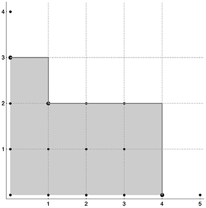
Figure 1. Set $\hat{{W}}$ in Example 2.2.1.

3. Prony-Type Polynomials

3.1. The Polynomials

Let f : ℤ² → ℂ be an N-sparse bivariate exponential sum with parameters z₁, …, z_N, and coefficients a₁, a₂, …, a_N ∈ ℂ\{0}

$\begin{array}{ll}f(\text{n})={\displaystyle \sum _{j=1}^N}{a}_j{\text{z}}_j^{\text{n}}={\displaystyle \sum _{j=1}^N}{a}_j{z}_{j,1}^{n_1}{z}_{j,2}^{n_2}.& (12)\end{array}$

Since f depends on n, we consider f as a bi-variate sequence f(n) = f_{n1, n2}. Let us remark, that further in the paper the number N ∈ ℤ₊ will always denote the number of parameters in (12), and we assume it to be known. In the two-dimensional case using f we build an analog of the Toeplitz matrix mentioned in the original Prony algorithm. Namely, let us consider the matrix

$\begin{array}{l}{{T}}_N={\left(f_{l(k)-l(j),r(k)-r(j)}\right)}_{k,j=0}^{N-1}=\left(\begin{array}{cccc}{f}_{0,0}& f_{l(1)-l(0),r(1)-r(0)}& \cdots & f_{l(N-1)-l(0),r(N-1)-r(0)}\\ f_{l(0)-l(1),r(0)-r(1)}& f_{0,0}& \cdots & f_{l(N-1)-l(1),r(N-1)-r(1)}\\ ⋮& ⋮& \ddots & ⋮\\ f_{l(0)-l(k),r(0)-r(k)}& f_{l(1)-l(k),r(1)-r(k)}& \cdots & f_{l(N-1)-l(k),r(N-1)-r(k)}\\ ⋮& ⋮& \ddots & ⋮\\ f_{l(0)-l(N-1),r(0)-r(N-1)}& f_{l(1)-l(N-1),r(1)-r(N-1)}& \cdots & f_{0,0}\end{array}\right),\end{array}$

which we call the bivariate Toeplitz matrix or shortly bi-Toeplitz matrix of f-samples. The index set of the elements of ${{T}}_N$ we denote by

$\begin{array}{ll}{I}_N=\left\{\text{i}\in {\mathbb{Z}}^2:\text{i}=(l(k)-l(j),r(k)-r(j)\right),k,j=0,\dots ,N-1\}.& (13)\end{array}$

For the same N ∈ ℤ₊, we denote by

$\begin{array}{l}{\hat{\text{z}}}_N={\left({\text{z}}^{l(j),r(j)}\right)}_{j=0}^{N-1}={\left(z_1^{l(j)}{z}_2^{r(j)}\right)}_{j=0}^{N-1}\end{array}$

the row vector of monomials that obviously consists of the first N monomials from the row of ordered monomials (9).

The next object we consider is some set of elements from the integer grid $D_N\subset {\mathbb{Z}}_{+}^2$ defined in the following way:

$D_N=\left\{(l(j),r(j)):j=N,\dots ,N+l(N)+r(N)\right\}.$

The set D_N is called the degree set of f, and it consists of exponents we will use further for constructing Prony-type polynomials. For all vectors m = (m₁, m₂) ∈ D_N, let us denote by

$\begin{array}{l}{\text{f}}_{N,\text{m}}={\left(f_{\text{m}-(l(j),r(j))}\right)}_{j=0}^{N-1}={(f_{m_1-l(j),m_2-r(j)})}_{j=0}^{N-1}\end{array}$

the column vectors called the column vectors of additional samples. The set of indices of the vectors f_N,m for all m ∈ D_N we denote by

$\begin{array}{ll}{I}_N^{+}=\left\{\text{i}\in {\mathbb{Z}}^2:\text{i}=\text{m}-(l(j),r(j)),\text{m}\in D_N,j=0,\dots ,N-1\right\},& (14)\end{array}$

which we call an additional index set.

Definition 3.1.1. Given an N-sparse bivariate exponential sum f, for all m ∈ D_N we define Prony-type polynomials as determinants of the following block matrices:

From the cardinality of D_N, it follows that there are exactly l(N) + r(N) + 1 polynomials $P_N^{\text{m}}$ for the N-sparse f. Moreover, the total degree of such polynomials can differ by one. Rewriting $N=\frac{n(n+1)}{2}+i$ in terms of n ∈ ℤ₊ and 0 ≤ i ≤ n (see (10)), provides some additional information about the number of Prony-type polynomials of a certain total degree

$\begin{array}{l}\#\{\text{m}\in D_N:\text{ TD}(P_N^{\text{m}})=l(N)+r(N)\}=n+1-i,\\ \#\{\text{m}\in D_N:\text{ TD}(P_N^{\text{m}})=l(N)+r(N)+1\}=i.\end{array}$

Theorem 3.1.1. Let f : ℤ² → ℂ be an N-sparse exponential sum of the form

$\begin{array}{l}f(\text{n})={\displaystyle \sum _{j=1}^N}{a}_{j}exp(-\text{i}\langle {\omega }_j,\text{n}\rangle )={\displaystyle \sum _{j=1}^N}{a}_j{\text{z}}_j^{\text{n}},\end{array}$

with coefficients a_j ∈ ℂ\{0}and parameters ${\text{z}}_j\in T^2,j=1,\dots ,N$, where the number of parameters N has the representation $N=\frac{n(n+1)}{2}+i,$ for some n ∈ ℤ₊ and 0 ≤ i ≤ n. Besides, let D_N be the degree set

$D_N=\left\{(l(j),r(j)):j=N,\dots ,N+l(N)+r(N)\right\}.$

and, for all m ∈ D_N, let $P_N^{\text{m}}$ be the corresponding Prony-type polynomials

If the parameters z_j, j = 1, …, N, are pairwise distinct with at least n pairwise distinct components, namely, for ℓ = 1, 2, z_{jp, ℓ} ≠ z_{kp, ℓ} if j_p ≠ k_p, p = 1, …, n, then the parameters z_j, j = 1, …, N, form the set of common zeros of the polynomial set ${{P}}_N=\langle P_N^{\text{m}}:\text{m}\in D_N\rangle$.

Proof. (A) First of all, we prove that the parameters z₁, z₂, …, z_N belong to the set of common zeros of Prony-type polynomials, i.e., $P_N^{\text{m}}({\text{z}}_j)=0$, for all j = 1, …, N, and all m ∈ D_N.

Assuming that f : ℤ² → ℂ is an N-sparse bivariate exponential sum with parameters ${\text{z}}_1,\dots ,{\text{z}}_N\in T^2$ and coefficients a₁, a₂, …, a_N ∈ ℂ\{0}, we construct the degree set

$D_N=\left\{(l(j),r(j)):j=N,\dots ,N+l(N)+r(N)\right\}.$

Taking some m = (m₁, m₂) ∈ D_N, we represent the corresponding Prony-type polynomial $P_N^{\text{m}}$ in the following form:

$\begin{array}{l}{P}_N^{\text{m}}(\text{z})=\frac{1}{det{{T}}_N}{\Delta }_N^{\text{m}}(\text{z}),\end{array}$

where

$\begin{array}{l}{\Delta }_N^{\text{m}}(\text{z})=\left|\begin{array}{cccc}{f}_{0,0}& \cdots & f_{l(N-1),r(N-1)}& f_{m_1,m_2}\\ f_{-1,0}& \cdots & f_{l(N-1)-1,r(N-1)}& f_{m_1-1,m_2}\\ ⋮& \ddots & ⋮& ⋮\\ f_{-l(N-1),-r(N-1)}& \cdots & f_{0,0}& f_{m_1-l(N-1),m_2-r(N-1)}\\ 1& \cdots & {\text{z}}^{(l(N-1),r(N-1))}& {\text{z}}^{\text{m}}\end{array}\right|.\end{array}$

Owing to the definition of the exponential sum f(n), we have

$\begin{array}{l}{\Delta }_N^{\text{m}}(\text{z})=\left|\begin{array}{cccc}{\displaystyle \sum _{j=1}^N}{a}_j{\text{z}}_j^{(0,0)}& {\displaystyle \sum _{j=1}^N}{a}_j{\text{z}}_j^{(1,0)}& \cdots & {\displaystyle \sum _{j=1}^N}{a}_j{\text{z}}_j^{(m_1,m_2)}\\ {\displaystyle \sum _{j=1}^N}{a}_j{\text{z}}_j^{(-1,0)}& {\displaystyle \sum _{j=1}^N}{a}_j{\text{z}}_j^{(0,0)}& \cdots & {\displaystyle \sum _{j=1}^N}{a}_j{\text{z}}_j^{(m_1-1,m_2)}\\ ⋮& ⋮& \ddots & ⋮\\ {\displaystyle \sum _{j=1}^N}{a}_j{\text{z}}_j^{(-l(N-1),-r(N-1))}& {\displaystyle \sum _{j=1}^N}{a}_j{\text{z}}_j^{(-l(N-1)+1,-r(N-1))}& \cdots & {\displaystyle \sum _{j=1}^N}{a}_j{\text{z}}_j^{(m_1-l(N-1),m_2-r(N-1))}\\ 1& {\text{z}}^{(1,0)}& \cdots & {\text{z}}^{\text{m}}\end{array}\right|.\end{array}$

Applying multi-linearity of determinants to the first row of ${\Delta }_N^{\text{m}}(\text{z})$, we can rewrite ${\Delta }_N^{\text{m}}(\text{z})$ as the sum of N determinants

$\begin{array}{l}{\Delta }_N^{\text{m}}(\text{z})=={\displaystyle \sum _{i_1=1}^N}\left|\begin{array}{cccc}{a}_{i_1}{\text{z}}_{i_1}^{(0,0)}& a_{i_1}{\text{z}}_{i_1}^{(1,0)}& \cdots & a_{i_1}{\text{z}}_{i_1}^{(m_1,m_2)}\\ {\displaystyle \sum _{j=1}^N}{a}_j{\text{z}}_j^{(-1,0)}& {\displaystyle \sum _{j=1}^N}{a}_j{\text{z}}_j^{(0,0)}& \cdots & {\displaystyle \sum _{j=1}^N}{a}_j{\text{z}}_j^{(m_1-1,m_2)}\\ ⋮& ⋮& \ddots & ⋮\\ {\displaystyle \sum _{j=1}^N}{a}_j{\text{z}}_j^{(-l(N-1),-r(N-1))}& {\displaystyle \sum _{j=1}^N}{a}_j{\text{z}}_j^{(-l(N-1)+1,-r(N-1))}& \cdots & {\displaystyle \sum _{j=1}^N}{a}_j{\text{z}}_j^{(m_1-l(N-1),m_2+r(N-1))}\\ 1& {\text{z}}^{(1,0)}& \cdots & {\text{z}}^{(m_1,m_2)}\end{array}\right|.\end{array}$

Repeating this process up to the penultimate row of the determinant ${\Delta }_N^{\text{m}}(\text{z})$, we represent this determinant as a certain combination of sums

$\begin{array}{ll}{P}_N^{\text{m}}(\text{z})=\frac{1}{det{{T}}_N}{\displaystyle \sum _{i_1=1}^N}{\displaystyle \sum _{i_2=1}^N}\dots {\displaystyle \sum _{i_N=1}^N}{\Delta }_{(i_1,i_2,\dots ,i_N)}^{\text{m}}(\text{z}),& (16)\end{array}$

where

$\begin{array}{l}{\Delta }_{(i_1,i_2,\dots ,i_N)}^{\text{m}}(\text{z})=\\ \left|\begin{array}{cccc}{a}_{i_1}{\text{z}}_{i_1}^{(0,0)}& a_{i_1}{\text{z}}_{i_1}^{(1,0)}& \cdots & a_{i_1}{\text{z}}_{i_1}^{(m_1,m_2)}\\ a_{i_2}{\text{z}}_{i_2}^{(-1,0)}& a_{i_2}{\text{z}}_{i_2}^{(0,0)}& \cdots & a_{i_2}{\text{z}}_{i_2}^{(m_1-1,m_2)}\\ ⋮& ⋮& \ddots & ⋮\\ a_{i_N}{\text{z}}_{i_N}^{(-l(N-1),-r(N-1))}& a_{i_N}{\text{z}}_{i_N}^{(-l(N-1)+1,-r(N-1))}& \cdots & a_{i_N}{\text{z}}_{i_N}^{(m_1-l(N-1),m_2-r(N-1))}\\ 1& {\text{z}}^{(1,0)}& \cdots & {\text{z}}^{(m_1,m_2)}\end{array}\right|.\end{array}$

Among all the determinants ${\Delta }_{(i_1,i_2,\dots ,i_N)}^{\text{m}}(\text{z})$ there are two types:

I.: determinants with at least two equal indices i_q and i_p, for some q ≠ p, 0 ≤ q, p ≤ N;

II.: determinants where all indices i_k, k = 1, …, N, are different.

Let us consider the determinants of type I. We assume that for some q ≠ p, 0 ≤ q, p ≤ N, some indices i_q and i_p coincide, for example, $i_q=i_p=i^{\prime }$. In this case the determinant ${\Delta }_{(i_1,i_2,\dots ,i_N)}^{\text{m}}(\text{z})$ vanishes, namely

$\begin{array}{l}{{\Delta }^{\text{m}}}_{(i_1,i_2,\dots ,i_N),\text{typeI}}(\text{z})\\ =\left|\begin{array}{cccc}⋮& ⋮& \ddots & ⋮\\ a_{i_q}{\text{z}}_{i_q}^{(-l(q),-r(q))}& a_{i_q}{\text{z}}_{i_q}^{(-l(q)+1,-r(q))}& \cdots & a_{i_q}{\text{z}}_{i_q}^{(k+l(q),m+r(q))}\\ ⋮& ⋮& \ddots & ⋮\\ a_{i_p}{\text{z}}_{i_p}^{(-l(p),-r(p))}& a_{i_p}{\text{z}}_{i_p}^{(-l(p)+1,-r(p))}& \cdots & a_{i_p}{\text{z}}_{i_p}^{(k-l(p),m-r(p))}\\ ⋮& ⋮& \ddots & ⋮\\ 1& {\text{z}}^{(1,0)}& \cdots & {\text{z}}^{(k,m)}\end{array}\right|\\ ={\text{z}}_{i^{\prime }}^{(-l(p)+l(q),-r(p)+r(q))}\left|\begin{array}{ccc}⋮& \ddots & ⋮\\ a_{i^{\prime }}{\text{z}}_{i^{\prime }}^{(-l(q),-r(q))}& \cdots & a_{i^{\prime }}{\text{z}}_{i^{\prime }}^{(k-l(q),m-r(q))}\\ ⋮& \ddots & ⋮\\ a_{i^{\prime }}{\text{z}}_{i^{\prime }}^{(-l(q),-r(q))}& \cdots & a_{i^{\prime }}{\text{z}}_{i^{\prime }}^{(k-l(q),m-r(q))}\\ ⋮& \ddots & ⋮\\ 1& \cdots & {\text{z}}^{(k,m)}\end{array}\right|\\ =0.\end{array}$

Consequently, in the representation (16) nonzero terms are just determinants ${\Delta }_{(i_1,i_2,\dots ,i_N)}^{\text{m}}(\text{z})$ with pairwise distinct i_k, k = 1, …, N. Hence,

$\begin{array}{ll}{P}_N^{\text{m}}(\text{z})=\frac{1}{det{{T}}_N}{\displaystyle \sum _{\begin{array}{c}{i}_1,i_2\dots i_N=1\\ i_j\ne i_k,k\ne j\end{array}}^N}{\Delta }_{(i_1,i_2,\dots ,i_N)}(\text{z}).& (17)\end{array}$

Let us consider the value $P_N^{\text{m}}({\text{z}}_j)$ for some fixed parameter z_j, 1 ≤ j ≤ N, using (17). Since all the indices i₁, …i_N also run from 1 to N, the index j of the parameter z_j must coincide with some index i_s, 0 ≤ s ≤ N, and it results in the vanishing of $P_N^{\text{m}}({\text{z}}_j)$, since

$\begin{array}{l}{{\Delta }^{\text{m}}}_{(i_1,i_2,\dots ,i_N)}({\text{z}}_j)\\ =\left|\begin{array}{cccc}⋮& ⋮& \ddots & ⋮\\ a_{i_s}{\text{z}}_{i_s}^{(-l(q),-r(q))}& a_{i_s}{\text{z}}_{i_s}^{(-l(q)+1,-r(q))}& \cdots & a_{i_s}{\text{z}}_{i_s}^{(m_1-l(q),m_2-r(q))}\\ ⋮& ⋮& \ddots & ⋮\\ 1& {\text{z}}_j^{(1,0)}& \cdots & {\text{z}}_j^{(m_1,m_2)}\end{array}\right|\\ =a_j{\text{z}}_j^{(-l(q),-r(q))}\left|\begin{array}{cccc}⋮& ⋮& \ddots & ⋮\\ 1& {\text{z}}_j^{(1,0)}& \cdots & {\text{z}}_j^{(m_1,m_2)}\\ ⋮& ⋮& \ddots & ⋮\\ 1& {\text{z}}_j^{(1,0)}& \cdots & {\text{z}}_j^{(m_1,m_2)}\end{array}\right|\\ =0.\end{array}$

As the multidegree m = (m₁, m₂) ∈ D_N, the polynomial $P_N^{\text{m}}(\text{z})$ and the parameter z_j were arbitrarily chosen, it follows that Prony-type polynomials vanish at the points z₁, z₂, …, z_N, namely $P_N^{\text{m}}({\text{z}}_j)=0$, for all z_j, j = 1, …, N, and for all m ∈ D_N.

(B) Now let us show that the set of Prony-type polynomials ${{P}}_N=\left\{P_N^{\text{m}}(\text{z}):\text{m}\in D_N\right\}$ can not have more than N common zeros.

Let N ∈ ℤ₊ be, as previously, the number of parameters and ${{P}}_N$ be the set of the Prony-type polynomials, ${{P}}_N=\left\{P_N^{\text{m}}:\text{m}\in D_N\right\}$. By ${{I}}_N$ we denote the ideal generated by ${{P}}_N$, ${{I}}_N=\langle {{P}}_N\rangle$. In the first part of the proof we have shown that having N parameters a lower bound for the number of common zeros of Prony-type polynomials is N. To find an upper bound for the cardinality of the variety ${V}({{P}}_N)$, we will use Lemma 2.2.1 and the fact that for any ideal ${I}$ generated by the set of polynomials P = {p₁, …, p_k} it holds $\langle \text{LT}({I})\rangle \supseteq \langle \text{LT}(p_1),\dots ,\text{LT}(p_k)\rangle$.

Let us start with the number of parameters N ∈ ℤ₊ that for some n ∈ ℤ₊ can be represented in the form

$\begin{array}{l}N=\frac{n(n+1)}{2}.\end{array}$

Then, the vector of Cantor inverse functions takes the value (l(N), r(N)) = (n, 0) and, obviously, l(N) + r(N) = n. Therefore, the degree set D_N consists of all the bivariate exponents of the total degree n,

$\begin{array}{l}{D}_N=\left\{(n,0),\dots ,(i,n-i),\dots ,(0,n)\right\}.\end{array}$

This means that there are n + 1 Prony-type polynomials and all of them are of total degree n. For this reason, all initial monomials for the ideal ${{I}}_N$ are among the monomials of the total degree less than or equal to n − 1. To visualize the sets of initial monomials, it is very convenient to use an integer grid [19], where each point denotes the exponent vector of the corresponding monomial. In Figure 2A, we illustrate the set of monomials of the total degree less than or equal to n − 1. According to (8), there are exactly $\frac{n(n+1)}{2}=N$ such monomials. Thus, there are at most N initial monomials. Lemma 2.2.1 tells us that, under above conditions, the number of points in ${V}({{I}}_N)$ is also at most N. This means that the Prony-type polynomials can have at most N common zeros in this case.

FIGURE 2

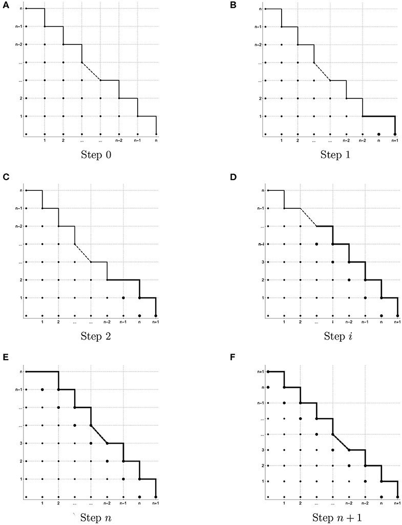
Figure 2. Illustration of sets of initial monomials. (A) Step 0, (B) Step 1, (C) Step 2, (D) Step i, (E) Step n, and (F) Step n + 1.

Now let for the same n ∈ ℤ₊ the number of parameters N ∈ ℤ₊ be of the form

$\begin{array}{l}N=\frac{n(n+1)}{2}+1.\end{array}$

In this case (l(N), r(N)) = (n − 1, 1), but the value l(N) + r(N) = n is still the same. Therefore, the degree set D_N also consists of n + 1 elements, however, in this case we start with the exponent (n − 1, 1) and end up with (n + 1, 0),

$\begin{array}{l}{D}_N=\left\{(n-1,1),\dots ,(i,n-i),\dots ,(0,n),(n+1,0)\right\}.\end{array}$

As a result, we have got one additional point on the integer grid (see Figure 2B) that corresponds to the monomial $z_1^{n+1}$. Hereupon, the upper bound for the number of potential initial monomials has been increased by one in comparison with the previous step. Namely, the set of potential initial monomials of ${{I}}_N$ belongs to the set consisting of monomials of total degree less than or equal to n − 1 and of the monomial $z_1^{n+1}$. Hence, the ideal ${{I}}_N$ generated by the Prony-type polynomials can have at most $\frac{n(n+1)}{2}+1=N$ initial monomials. However, with respect to Lemma 2.2.1 the number of common zeros of Prony-type polynomials cannot exceed the number of initial monomials. This means that the Prony-type polynomials can have at most $\frac{n(n+1)}{2}+1=N$ common zeros.

In the same way, for any $N=\frac{n(n+1)}{2}+i$, where 0 ≤ i ≤ n, we get that the number of initial monomials of ideal ${{I}}_N$ does not exceed $\frac{n(n+1)}{2}+i$ (see Figures 2C–E). Thus, the number of common zeros of the Prony-type polynomials is not exceeding $N=\frac{n(n+1)}{2}+i$.

In step n + 1, where

$\begin{array}{l}N=\frac{n(n+1)}{2}+n+1=\frac{(n+1)(n+2)}{2},\end{array}$

the vector of Cantor inverse functions takes the value (l(N), r(N)) = (n + 1, 0) and l(N) + r(N) = n + 1. For this reason, the degree set D_N consists of all the bivariate exponents of the total degree n + 1,

$\begin{array}{l}{D}_N=\left\{(n+1,0),\dots ,(i,n-i),\dots ,(0,n+1)\right\}\end{array}$

and there are n + 2 Prony-type polynomials (see Figure 2F). Hence, for such N all the initial monomials for ${{I}}_N$ belong to the set of monomials of total degree that does not exceed n + 1. Having $\frac{(n+1)(n+2)}{2}=N$ such monomials, we finish with at most N common zeros for the set of the Prony-type polynomials ${{P}}_N$. Taking $N=\frac{(n+1)(n+2)}{2}+i$, 0 ≤ i ≤ n + 1, we will repeat the previous scenario, but in this case with n + 2 steps. Since each integer number can be uniquely represented in the form (10), it follows that for arbitrary chosen N ∈ ℤ₊ the Prony-type polynomials $P_N^{\text{m}}$ for m ∈ D_N can have at most N common zeros. Moreover, in the first part of the proof it is pointed out that the common zeros are precisely the parameters z_j, j = 1, …, N. □

Remark. The Prony-type polynomials can be considered as some direct generalization of the univariate Prony polynomial (3).

Using notation $P_N^{(l(N+m),r(N+m))}=P_N^m$ for some integer m, let us rewrite the Prony-type polynomials, see Definition 3.1.1, $P_N^{\text{m}}$ for m ∈ D_N = {(l(j), r(j)) : j = N, …, N + l(N) + r(N)}, in the form

$P_N^m(\text{z})={\displaystyle \sum _{k=0}^{N-1}}{p}_{k,m}{\text{z}}^{(l(k),r(k))}+p_{N,m}{\text{z}}^{(l(N+m),r(N+m))},$

where the leading coefficient p_{N, m} = 1, m = 0, …, l(N) + r(N) according to Definition 3.1.1. Moreover, the remaining coefficients are defined as

$p_{k,m}=\frac{det{\displaystyle {{T}}_{N,k}^m}}{det{{T}}_N},$

where the matrix ${{T}}_{N,k}^m$ is the matrix formed by cutting out the k-th column of the bi-Toeplitz matrix ${{T}}_N$, ${{T}}_{N,k}={(f_{l(i)-l(j),r(i)-r(j)})}_{i,j=0,j\ne k}^{N-1}$, and appending to ${{T}}_{N,k}$ the column vector f_{N, m}: = f_{N,(l(N + m), r(N + m))}, namely

${{T}}_{N,k}^m=({{T}}_{N,k}\mid {\text{f}}_{N,m}).$

By Cramer's rule the coefficients of the polynomial $P_N^m$ are the solutions of the corresponding linear system of equations

$\begin{array}{ll}{{T}}_N{\text{p}}_m=-{\text{f}}_{N,m},& (18)\end{array}$

where ${{T}}_N={(f_{l(i)-l(j),r(i)-r(j)})}_{i,j=0}^{N-1}\in {ℂ}^{N\times N}$ is the bi-Toeplitz matrix, ${\text{f}}_{N,m}={\text{f}}_{N,(l(N+m),r(N+m))}={(f_{l(N+m)-l(j),r(N+m)-r(j)})}_{j=0}^{N-1}$ ∈ ℂ^N are the column vectors of the additional samples defined above, and ${\text{p}}_m={(p_{0,m},p_{1,m},\dots ,p_{N-1,m})}^{\text{T}}\in {ℂ}^N$ is the vector of the coefficients of a Prony-type polynomial $P_N^m$. It is easy to see that the linear systems of equations (18) provide the following properties of the coefficients p_{j, m}, j = 1, …, N, m = 0, …, l(N) + r(N),

$\begin{array}{l}{\displaystyle \sum _{k=0}^{N-1}}{p}_{k,m}{f}_{l(k)-l(q),r(k)-r(q)}+p_{N,m}{f}_{l(N+m)-l(q),r(N+m)-r(q)}\\ ={\displaystyle \sum _{j=1}^N}{a}_j{\text{z}}_j^{-(l(q),r(q))}{\displaystyle \sum _{k=0}^{N-1}}{p}_{k,m}{\text{z}}_j^{(l(k),r(k))}\\ +{\displaystyle \sum _{j=1}^N}{a}_j{\text{z}}_j^{-(l(q),r(q))}{p}_{N,m}{\text{z}}_k^{(l(N+m),r(N+m))}\\ ={\displaystyle \sum _{j=1}^N}{a}_j{\text{z}}_j^{-(l(q),r(q))}{P}_N^m({\text{z}}_j)=0,\end{array}$

for q = 0, …, N − 1 and m = 0, …, l(N) + r(N). It is obvious, that such properties of coefficients and the systems of equations (18) are similar to the properties (4) and the system (5) from the one-dimensional case.

Corollary 3.1.1. The Prony-type polynomials depend only on the parameters z_j, and they are invariant under a choice of the coefficients a_j, for j = 1, …, N.

Proof. From the representation (17) it follows, that as soon as all indices i_k for k = 1, …, N are pairwise distinct in the determinant ${\Delta }_{(i_1,i_2,\dots ,i_N)}^{\text{m}}(\text{z})$, we can rewrite it as

$\begin{array}{l}{{\Delta }^{\text{m}}}_{(i_1,i_2,\dots ,i_N)}(\text{z})\\ =\left|\begin{array}{ccc}{a}_{i_1}{\text{z}}_{i_1}^{(0,0)}& \cdots & a_{i_1}{\text{z}}_{i_1}^{(m_1,m_2)}\\ ⋮& \ddots & ⋮\\ a_{i_N}{\text{z}}_{i_N}^{(-l(N-1),-r(N-1))}& \cdots & a_{i_N}{\text{z}}_{i_N}^{(m_1-l(N-1),m_2-r(N-1))}\\ 1& \cdots & {\text{z}}^{(m_1,m_2)}\end{array}\right|\\ =a_1{a}_2\dots a_N\left|\begin{array}{ccc}{\text{z}}_{i_1}^{(0,0)}& \cdots & {\text{z}}_{i_1}^{(m_1,m_2)}\\ ⋮& \ddots & ⋮\\ {\text{z}}_{i_N}^{(-l(N-1),-r(N-1))}& \cdots & {\text{z}}_{i_N}^{(m_1-l(N-1),m_2-r(N-1))}\\ 1& \cdots & {\text{z}}^{(m_1,m_2)}\end{array}\right|\\ =a_1{a}_2\dots a_N{\tilde{\Delta }}_{(i_1,i_2,\dots ,i_N)}^{\text{m}}(\text{z}).\end{array}$

Using the same procedure for the determinant of the bi-Toeplitz matrix ${{T}}_N$, one gets a similar representation

$\begin{array}{l}det{{T}}_N=a_1{a}_2\dots a_N{\displaystyle \sum _{\begin{array}{c}{i}_1,i_2\dots i_N=1\\ i_j\ne i_k,k\ne j\end{array}}^N}{\tilde{\Delta }}_{(i_1,i_2,\dots ,i_N)},\end{array}$

where

$\begin{array}{l}{\tilde{\Delta }}_{(i_1,i_2,\dots ,i_N)}=\left|\begin{array}{ccc}{\text{z}}_{i_1}^{(0,0)}& \cdots & {\text{z}}_{i_1}^{l(N-1),r(N-1)}\\ {\text{z}}_{i_2}^{(-1,0)}& \cdots & {\text{z}}_{i_2}^{l(N-1)-1,r(N-1)}\\ ⋮& \ddots & ⋮\\ {\text{z}}_{i_N}^{(-l(N-1),-r(N-1))}& \cdots & {\text{z}}_{i_N}^{(0,0)}\end{array}\right|.\end{array}$

Such representations of determinants result in the mentioned properties of the Prony-type polynomials, namely

$\begin{array}{l}{P}_N^{\text{m}}(\text{z})=\frac{1}{det{{T}}_N}{\displaystyle \sum _{\begin{array}{c}{i}_1,i_2\dots i_N=1\\ i_j\ne i_k,k\ne j\end{array}}^N}{\Delta }_{(i_1,i_2,\dots ,i_N)}(\text{z}),\\ ={\left(a_1{a}_2\dots a_N{\displaystyle \sum _{\begin{array}{c}{i}_1,i_2\dots i_N=1\\ i_j\ne i_k,k\ne j\end{array}}^N}{\tilde{\Delta }}_{(i_1,i_2,\dots ,i_N)}\right)}^{-1}{a}_1{a}_2\dots a_N\\ {\displaystyle \sum _{\begin{array}{c}{i}_1,i_2\dots i_N=1\\ i_j\ne i_k,k\ne j\end{array}}^N}{\tilde{\Delta }}_{(i_1,i_2,\dots ,i_N)}^{\text{m}}(\text{z})\\ ={\displaystyle \sum _{\begin{array}{c}{i}_1,i_2\dots i_N=1\\ i_j\ne i_k,k\ne j\end{array}}^N}{\tilde{\Delta }}_{(i_1,i_2,\dots ,i_N)}^{\text{m}}(\text{z}){\left({\displaystyle \sum _{\begin{array}{c}{i}_1,i_2\dots i_N=1\\ i_j\ne i_k,k\ne j\end{array}}^N}{\tilde{\Delta }}_{(i_1,i_2,\dots ,i_N)}\right)}^{-1}.\end{array}$

□

3.2. PTP Algorithm

The results from the previous subsection provide the following computational algorithm that allows detecting the parameters and frequency vectors of the N-sparse bivariate exponential sum, we call this method PTP algorithm.

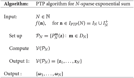
The number of samples of f required by the PTP algorithm is discussed in the lemma below.

Lemma 3.2.1. Let $N=\frac{n(n+1)}{2}+i$, for n ∈ ℤ₊, 0 ≤ i ≤ n, and I_N, $I_N^{+}$ be the sets defined in (13) and (14) respectively. The set of samples $I_{PTP}(N):=I_N\cup I_N^{+}$ required for the PTP algorithm satisfies

$\begin{array}{l}\#I_{PTP}(N)=\{\begin{array}{ll}6N-\frac{1}{2}(\sqrt{1+8(N-i)}+1)-4i,& i>0,\\ 6N+\frac{3}{2}(1-\sqrt{8N+1}),& i=0.\end{array}\end{array}$

Proof. Let N be an integer. The index set $I_N\subset {\mathbb{Z}}^2$ of the elements of the matrix ${{T}}_N$ fulfills by definition

$\begin{array}{l}\forall \text{k}\in I_N:-\text{k}\in I_N\wedge (-\text{k}=\text{k}\iff \text{k}=(0,0)).\end{array}$

Each element of I_N belongs to one of the four sets listed below:

$\begin{array}{l}{M}_1=\left\{(k_1,k_2)\in I_N:k_1+k_2\ge 1\right\},\\ M_2=\left\{(k_1,k_2)\in I_N:k_1+k_2\le -1\right\}=\left\{\text{k}\in I_N:-\text{k}\in M_1\right\},\\ M_3=\left\{(k_1,k_2)\in I_N:k_1+k_2=0\wedge k_1\ge 0\right\},\\ M_4=\left\{(k_1,k_2)\in I_N:k_1+k_2=0\wedge k_2\ge 0\right\}\\ =\left\{\text{k}\in I_N:-\text{k}\in M_3\right\}.\end{array}$

Moreover, the zero vector (0, 0) is in the set M₃ and in the set M₄, simultaneously. However, all the other elements k ∈ I_N are exactly in one of the sets M₁, M₂, M₃, M₄. Consequently, we get

$\begin{array}{l}{I}_N^{\star }=M_1\cup M_3\\ =\left\{(k_1,k_2)\in I_N:k_1+k_2\ge 1\vee k_1+k_2=0\wedge k_1\ge 0\right\},\end{array}$

and

$\begin{array}{c}{I}_N=I_N^{\star }\cup \left\{-\text{k}:\text{k}\in I_N^{\star }\right\}\\ I_N^{\star }\cap \left\{-\text{k}:\text{k}\in I_N^{\star }\right\}=\left\{(0,0)\right\}.\end{array}$

This allows us to compute the cardinality of the set I_N in terms of the cardinality of $I_N^{\star }$, namely

$\begin{array}{l}\#I_N=2\#I_N^{\star }-1.\end{array}$

Finally, to compute all the samples that are required by the PTP algorithm we can use the equality

$\begin{array}{l}\#I_N\cup I_N^{+}=\#I_N+\#I_N^{+}\backslash I_N=2\#I_N^{\star }-1+\#I_N^{+}\backslash I_N.\end{array}$

Now the aim is to find the number of elements of $I_N^{\star }$ und $I_N^{+}\backslash I_N$ for given N ∈ ℕ. As it has been mentioned before, each integer number N can be represented as $N=\frac{n(n+1)}{2}+i$, where n ∈ ℤ₊ and 0 ≤ i ≤ n. Carrying out the transformation

$\begin{array}{l}N=\frac{n(n+1)}{2}+i\iff n^2+n+2(i-N)=0\\ \iff n=\frac{1}{2}(\sqrt{1+8(N-i)}-1)\end{array}$

will help us later to formulate the result.

Let us start with $N=\frac{n(n+1)}{2}$ for some n ∈ ℕ, then l(N), r(N) = (n, 0). Consequently, the set I_N consists of all differences of tuples k, n ∈ ℤ _{+ ,<(n, 0)}, where the set ${\mathbb{Z}}_{+,<\text{n}}^2$ is defined as

$\begin{array}{l}{\mathbb{Z}}_{+,<\text{n}}^2=\left\{\text{k}\in {\mathbb{Z}}_{+}^2:\text{k}{<}_{\text{grlex}}\text{n}\right\}.\end{array}$

To compute the cardinality of $I_N^{\star }$, we decompose this set into disjoint subsets, where the number of elements is easier to compute. As the first subset of $I_N^{\star }$ we consider the set that consists only of integer vectors with non-negative components. We denote this set as

$\begin{array}{l}{I}_{N,{\mathbb{Z}}_{+}^2}^{\star }=\left\{(k_1,k_2)\in I_N^{\star }:k_1,k_2\ge 0\right\}=\left\{(0,0),(1,0),\dots ,(0,n-1)\right\}.\end{array}$

It is easy to see that the set $I_{N,{\mathbb{Z}}_{+}^2}^{\star }$ is exactly the exponent set of the monomials at the positions 0, 1, …, $\frac{n(n+1)}{2}-1=N-1$ in (9), and therefore it has exactly N elements. The remaining vectors $(k_1,k_2)\in I_N^{\star }$ need to have either k₁ < 0 or k₂ < 0. With respect to the definition of $I_N^{\star }$ one gets, on the one hand, that if k₁ < 0 then k₂ > −k₁. On the other hand, for k₂ < 0 it follows that k₁ ≥ −k₂. First of all, let us consider the vectors (k₁, k₂) of $I_N^{\star }$ with the negative second component. In this case k₂ can be one of the numbers −1, −2, …, −(n − 1). Consequently, all these elements belong to one of the disjoint sets

$\begin{array}{l}{I}_{N,k_2=-1}^{\star }=\left\{\text{k}=(k_1,k_2)\in I_N^{\star }:k_2=-1\right\}\\ =\left\{(1,-1),(2,-1),\dots ,(n-1,-1)\right\},\\ I_{N,k_2=-2}^{\star }=\left\{\text{k}=(k_1,k_2)\in I_N^{\star }:k_2=-2\right\}\\ =\left\{(2,-2),(3,-2),\dots ,(n-1,-2)\right\},\\ ⋮\\ I_{N,k_2=-(n-1)}^{\star }=\left\{\text{k}=(k_1,k_2)\in I_N^{\star }:k_2=-(n-1)\right\}\\ =\left\{(n-1,-(n-1))\right\}.\end{array}$

The cardinality of these sets is easy to compute, namely

$\begin{array}{l}\#I_{N,k_2=-p}^{\star }=n-p,p=1,\dots ,n-1.\end{array}$

Now let us consider the elements of $I_N^{\star }$ which have not yet been included in any of the previously mentioned subsets. These are the vectors $(k_1,k_2)\in I_N^{\star }$ with a negative first component. Then, such elements need to belong to one of the sets defined below

$\begin{array}{l}{I}_{N,k_1=-1}^{\star }=\left\{\text{k}=(k_1,k_2)\in I_N^{\star }:k_1=-1\right\}\\ =\left\{(-1,2),(-1,3),\dots ,(-1,n-1)\right\},\\ I_{N,k_1=-2}^{\star }=\left\{\text{k}=(k_1,k_2)\in I_N^{\star }:k_1=-2\right\}\\ =\left\{(-2,3),(-2,4),\dots ,(-2,n-1)\right\},\\ ⋮\\ I_{N,k_1=-(n-2)}^{\star }=\left\{\text{k}=(k_1,k_2)\in I_N^{\star }:k_1=-(n-2)\right\}\\ =\left\{(-(n-2),n-1)\right\}.\end{array}$

Also for these sets it is easy to deal with the number of elements,

$\begin{array}{l}\#I_{N,k_1=-p}^{\star }=n-p-1,p=1,\dots ,n-2.\end{array}$

All these sets have been constructed to make a partition of $I_N^{\star }$. As a result, for the cardinality of $I_N^{\star }$ one gets the representation

$\begin{array}{l}\#I_N^{\star }=\#I_{N,{\mathbb{Z}}_{+}^2}^{\star }+{\displaystyle \sum _{i=1}^{n-2}}\#I_{N,k_1=-i}^{\star }+{\displaystyle \sum _{i=1}^{n-1}}\#I_{N,k_2=-i}^{\star }\\ =\frac{n(n+1)}{2}+{\displaystyle \sum _{i=1}^{n-2}}(n-i-1)+{\displaystyle \sum _{i=1}^{n-1}}(n-i)\\ =\frac{n(n+1)}{2}+{\displaystyle \sum _{i=1}^{n-2}}i+{\displaystyle \sum _{i=1}^{n-1}}i\\ =\frac{n(n+1)}{2}+\frac{(n-2)(n-1)}{2}+\frac{(n-1)n}{2}\\ =\frac{1}{2}(3n^2-3n+2).& (19)\end{array}$

Finally, let us determine the cardinality of $I_N^{+}\backslash I_N$, i.e., the number of additional samples, for which we need to compute the vectors f_N,m, m ∈ D_N, that have not yet appeared in I_N. For $N=\frac{n(n+1)}{2}$ the degree set D_N consists of all $\text{k}=(k_1,k_2)\in {\mathbb{Z}}_{+}^2$ with |k| = n. Consequently, for each element m ∈ D_N there exists some 0 ≤ i < n, such that m = (n − i, i). According to the definition, the set $I_N^{+}$ consists of all vectors m − n where m ∈ D_N and $\text{n}\in {\mathbb{Z}}_{+,<(n,0)}^2$. To check which of these vectors are already in I_N, i.e. in the set of all the differences k − n where $\text{k},\text{n}\in {\mathbb{Z}}_{+,<(n,0)}^2$, let us analyze all possible cases:

(1) Let m = (n, 0) ∈ D_N and $\text{n}=(n_1,n_2)\in {\mathbb{Z}}_{+,<(n,0)}^2$. Then, for n = (n₁, n₂) with n₁ > 0 one has

$\begin{array}{l}\text{m}-\text{n}={\displaystyle \underset{\in {\mathbb{Z}}_{+,<(n,0)}^2}{{\displaystyle \underbrace{(n-1,0)}}}}-{\displaystyle \underset{\in {\mathbb{Z}}_{+,<(n,0)}^2}{{\displaystyle \underbrace{(n_1-1,n_2)}}}}\in I_N.\end{array}$

However, if n₁ = 0, then the element m − n = (n, −n₂) does not belong to I_N, and, therefore, it is in the set $I_N^{+}\backslash I_N$.

(2) Let m = (0, n) ∈ D_N and $\text{n}=(n_1,n_2)\in {\mathbb{Z}}_{+,<(n,0)}^2$. Then, for n = (n₁, n₂) with n₂ > 0 one has

$\begin{array}{l}\text{m}-\text{n}={\displaystyle \underset{\in {\mathbb{Z}}_{+,<(n,0)}^2}{{\displaystyle \underbrace{(0,n-1)}}}}-{\displaystyle \underset{\in {\mathbb{Z}}_{+,<(n,0)}^2}{{\displaystyle \underbrace{(n_1,n_2-1)}}}}\in I_N.\end{array}$

However, if n₂ = 0, then m − n = (−n₁, n) is located in the set $I_N^{+}\backslash I_N$.

(3) Let m ∈ D_N be of the form m = (n − i, i), where 0 < i < n and $\text{n}=(n_1,n_2)\in {\mathbb{Z}}_{+,<(n,0)}^2$. Then, for n = (n₁, n₂) with n₂ > 0 one has

$\begin{array}{l}\text{m}-\text{n}={\displaystyle \underset{\in {\mathbb{Z}}_{+,<(n,0)}^2}{{\displaystyle \underbrace{(n-i,i-1)}}}}-{\displaystyle \underset{\in {\mathbb{Z}}_{+,<(n,0)}^2}{{\displaystyle \underbrace{(n_1,n_2-1)}}}}\in I_N.\end{array}$

If n₂ = 0 and n₁ > 0 simultaneously, then

$\begin{array}{l}\text{m}-\text{n}={\displaystyle \underset{\in {\mathbb{Z}}_{+,<(n,0)}^2}{{\displaystyle \underbrace{(n-i-1,i)}}}}-{\displaystyle \underset{\in {\mathbb{Z}}_{+,<(n,0)}^2}{{\displaystyle \underbrace{(n_1-1,0)}}}}\in I_N.\end{array}$

However, in case n₁ = n₂ = 0 the vector m − n = m is an element of $I_N^{+}\backslash I_N$.

Hereby, we identify all $\text{k}\in I_N^{+}\backslash I_N$ and get the representation

$\begin{array}{r}{I}_N^{+}\backslash I_N=D_N\cup \left\{(n,-1),(n,-2),\dots ,(n,-(n-1))\right\}\\ \cup \left\{(-1,n),(-2,n),\dots ,(-(n-1),n)\right\},\end{array}$

which means that

$\begin{array}{ll}\#I_N^{+}\backslash I_N=3n-1.& (20)\end{array}$

Together with (19), it provides the number of all required samples, namely

$\begin{array}{ll}\#I_N\cup I_N^{+}=3n^2.& (21)\end{array}$

In terms of N we can represent the number of samples (21) as

$\begin{array}{l}\#I_N\cup I_N^{+}=6N+\frac{3}{2}(1-\sqrt{8N+1}).\end{array}$

Now let us consider the case, when N ∈ ℕ is of the form $N=\frac{n(n+1)}{2}+i$, where n ∈ ℤ₊ and 1 ≤ i ≤ n. Owing to l(N), r(N) = (n − i, i), the set I_N consists of all vectors k − n where $\text{k},\text{n}\in {\mathbb{Z}}_{+,<(n-i,i)}^2$. In this case the subset $I_{N,{\mathbb{Z}}_{+}^2}^{\star }$ of $I_N^{\star }$ has the structure

$\begin{array}{l}{I}_{N,{\mathbb{Z}}_{+}^2}^{\star }=\left\{(0,0),(1,0),\dots ,(0,n-1),(n,0),\dots ,(n-i+1,i-1)\right\}\end{array}$

and therefore the cardinality of $I_{N,{\mathbb{Z}}_{+}^2}^{\star }$ for such number N is $\#I_{N,{\mathbb{Z}}_{+}^2}^{\star }=\frac{n(n+1)}{2}+i$. Similar to the case considered before, we make the partition of $I_N^{\star }$ using the set $I_{N,{\mathbb{Z}}_{+}^2}^{\star }$ and the following sets

$\begin{array}{l}{I}_{N,k_2=-1}^{\star }=\left\{(1,-1),(2,-1),\dots ,(n,-1)\right\},\\ I_{N,k_2=-2}^{\star }=\left\{(2,-2),(3,-2),\dots ,(n,-2)\right\},\\ ⋮\\ I_{N,k_2=-(n-1)}^{\star }=\left\{(n-1,-(n-1)),(n,-(n-1))\right\}\end{array}$

and

$\begin{array}{l}{I}_{N,k_1=-1}^{\star }=\left\{(-1,2),(-1,3),\dots ,(-1,n-1)\right\},\\ I_{N,k_1=-2}^{\star }=\left\{(-2,3),(-2,4),\dots ,(-2,n-1)\right\},\\ ⋮\\ I_{N,k_1=-(n-2)}^{\star }=\left\{(-(n-2),n-1)\right\}.\end{array}$

Apparently, for the cardinality of the above listed sets it holds

$\begin{array}{l}\#I_{N,k_2=-p}^{\star }=n-p+1,p=1,\dots ,n-1\\ \#I_{N,k_1=-p}^{\star }=n-p-1,p=1,\dots ,n-2.\end{array}$

As a result, it is easy to compute the number of elements of $I_N^{\star }$

$\begin{array}{l}\#I_N^{\star }=\#I_{N,{\mathbb{Z}}_{+}^2}^{\star }+{\displaystyle \sum _{i=1}^{n-2}}\#I_{N,k_1=-i}^{\star }+{\displaystyle \sum _{i=1}^{n-1}}\#I_{N,k_2=-i}^{\star }=\frac{1}{2}(3n^2-n)+i.\end{array}$

Now it remains to clarify, how many new elements we have in $I_N^{+}\backslash I_N$, i.e. how many vectors m − n with m ∈ D_N and $\text{n}\in {\mathbb{Z}}_{+,<(n-i,i)}^2$ there exist, such that they have not yet appeared in I_N. For $N=\frac{n(n+1)}{2}+i$, where 1 ≤ i ≤ n, the set D_N is of the form

$\begin{array}{l}{D}_N=\left\{(n-i,i),\dots ,(0,n),(n+1,0),\dots ,(n+2-i,i-1)\right\}.\end{array}$

To answer the above question, let us consider all possible cases:

(1) Let m = (0, n) ∈ D_N and $\text{n}=(n_1,n_2)\in {\mathbb{Z}}_{+,<(n-i,i)}^2$. Then, for n = (n₁, n₂) with n₂ > 0 one has

$\begin{array}{l}\text{m}-\text{n}={\displaystyle \underset{\in {\mathbb{Z}}_{+,<(n-i,i)}^2}{{\displaystyle \underbrace{(0,n-1)}}}}-{\displaystyle \underset{\in {\mathbb{Z}}_{+,<(n-i,i)}^2}{{\displaystyle \underbrace{(n_1,n_2-1)}}}}\in I_N.\end{array}$

However, if n₂ = 0, then m − n = (−n₁, n) is not located in the set I_N.

(2) Let m = (m₁, m₂) ∈ D_N with |m| = n and m ≠ (0, n). If additionally $\text{n}=(n_1,n_2)\in {\mathbb{Z}}_{+,<(n-i,i)}^2$ with n₂ > 0, then it holds

$\begin{array}{l}\text{m}-\text{n}={\displaystyle \underset{\in {\mathbb{Z}}_{+,<(n-i,i)}^2}{{\displaystyle \underbrace{(m_1,m_2-1)}}}}-{\displaystyle \underset{\in {\mathbb{Z}}_{+,<(n-i,i)}^2}{{\displaystyle \underbrace{(n_1,n_2-1)}}}}\in I_N.\end{array}$

In the same way, for all n₂ = 0 and n₁ > 0 it holds

$\begin{array}{l}\text{m}-\text{n}={\displaystyle \underset{\in {\mathbb{Z}}_{+,<(n-i,i)}^2}{{\displaystyle \underbrace{(m_1-1,m_2)}}}}-{\displaystyle \underset{\in {\mathbb{Z}}_{+,<(n-i,i)}^2}{{\displaystyle \underbrace{(n_1-1,n_2)}}}}\in I_N.\end{array}$

However, if n₁ = n₂ = 0, then the difference m − n = m is not in the set I_N.

(3) Let m = (n + 1, 0) ∈ D_N, then for $\text{n}=(n_1,n_2)\in {\mathbb{Z}}_{+,<(n-i,i)}^2$ with n₁ > 0 one has

$\begin{array}{l}\text{m}-\text{n}={\displaystyle \underset{\in {\mathbb{Z}}_{+,<(n-i,i)}^2}{{\displaystyle \underbrace{(n,0)}}}}-{\displaystyle \underset{\in {\mathbb{Z}}_{+,<(n-i,i)}^2}{{\displaystyle \underbrace{(n_1-1,n_2)}}}}\in I_N.\end{array}$

If n₁ = 0, then m − n = (n + 1, −n₂) is not in the set I_N.

(4) Let m ∈ D_N with |m| = n + 1 and m ≠ (n + 1, 0). This means that all the vectors are of the form (n + 2 − j, j − 1), j = 2, 3, …, i. Then, for all $\text{n}=(n_1,n_2)\in {\mathbb{Z}}_{+,<(n-i,i)}^2$ with n₁ > 0 it holds

$\begin{array}{l}\text{m}-\text{n}={\displaystyle \underset{\in {\mathbb{Z}}_{+,<(n-i,i)}^2}{{\displaystyle \underbrace{(n+1-j,j-1)}}}}-{\displaystyle \underset{\in {\mathbb{Z}}_{+,<(n-i,i)}^2}{{\displaystyle \underbrace{(n_1-1,n_2)}}}}\in I_N.\end{array}$

If n₁ = 0 and n₂ > 0, then likewise

$\begin{array}{l}\text{m}-\text{n}={\displaystyle \underset{\in {\mathbb{Z}}_{+,<(n-i,i)}^2}{{\displaystyle \underbrace{(n+2-j,j-2)}}}}-{\displaystyle \underset{\in {\mathbb{Z}}_{+,<(n-i,i)}^2}{{\displaystyle \underbrace{(n_1,n_2-1)}}}}\in I_N.\end{array}$

Finally, if n₁ = n₂ = 0, m − n = m does not belong to I_N.

Having analyzed all cases, we can identify all elements of $\text{k}\in I_N^{+}\backslash I_N$,

$\begin{array}{l}{I}_N^{+}\backslash I_N=D_N\cup \left\{(-1,n),(-2,n),\dots ,(-n,n)\right\}\\ \cup \left\{(n+1,-1),(n+1,-2),\dots ,(n+1,n-1)\right\}\end{array}$

and the computation of its cardinality results in

$\begin{array}{ll}\#I_N^{+}\backslash I_N=3n.& (22)\end{array}$

Altogether it gives us the total number of required samples in the case when N ∈ ℕ is of the form $N=\frac{n(n+1)}{2}+i$, n ∈ ℤ₊, 1 ≤ i ≤ n,

$\begin{array}{ll}\#I_N\cup I_N^{+}=3n^2+2(n+i)-1.& (23)\end{array}$

We can rewrite the obtained result in terms of N in the following way

$\begin{array}{l}\#I_N\cup I_N^{+}=6N-\frac{1}{2}(\sqrt{1+8(N-i)}+1)-4i.\end{array}$

Combining all considered cases together, we have the total number of samples

$\begin{array}{l}\#I_{PTP}(N)=\{\begin{array}{ll}6N-\frac{1}{2}(\sqrt{1+8(N-i)}+1)-4i,& i>0,\\ 6N+\frac{3}{2}(1-\sqrt{8N+1}),& i=0.\end{array}\end{array}$

□

For example, Figure 3 illustrates the case when the number of parameters N = 4. In this case the sample set I_PTP(4) includes 17 elements, and consists of the index set I₄, of the extended samples set $I_4^{+}$ and of the degree set D₄. In general, the PTP algorithm requires ${O}(6N)$ f-samples what places the algorithm in terms of sample requirements between the method proposed in Cuyt and Wen-Shin [4] with the absolute minimum of samples (d + 1)N and the method from Kunis et al. [1] that requires at least (2N + 1)² evaluations of f. Sampling sets similar to the set I_PTP also have been considered in Josz et al. [17].

FIGURE 3

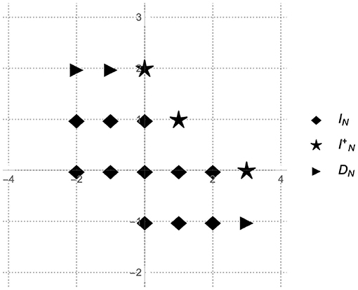
Figure 3. Sample set I_PTP(4).

4. Autocorrelation Sequence and Prony-Type Polynomials

As it was mentioned before, a certain disadvantage of the original Prony method is its instability in case when data are corrupted by noise. Since the Prony-type polynomials are a bi-variate generalization of the one-dimensional approach, the pure PTP-algorithm also inherits instability in noisy data case. Therefore, in this section we introduce the method based on the Prony-type polynomials and a windowed autocorrelation sequence that allows gaining more stability in case of noise corruption.

4.1. Localized Kernel

In this section, using the one-dimensional localized kernel constructed in Filbir et al. [5], we define a two-dimensional localized kernel and analyze its properties.

First of all let us introduce the necessary notations. For a Lebesgue measurable function F : ℝ → ℝ we use common notations

$\left|\right|F|{|}_{\infty }=\text{ess}{\displaystyle \underset{x\in ℝ}{sup}}|F(x)|,|\left|F\right|{|}_1={\displaystyle {\int }_{ℝ}}F(x)\text{d}x.$

Let S ≥ 2 be an integer and $\tilde{H}:ℝ\to \left[0,1\right]$ be an S times continuously differentiable function with the properties

$\begin{array}{l}\tilde{H}(t)=\tilde{H}(-t),\text{ for }t\in ℝ;\tilde{H}(t)=0,\text{ if }\left|t\right|\ge 1,\end{array}$

and bounded norm ${\tilde{H}}_1=\left|\right|\tilde{H}|{|}_1={\int }_{-1}^1\tilde{H}(t)\text{d}t$, $0<{\tilde{H}}_1<2$ (see [5]). Then, for some integer M ∈ ℕ we define a two-dimensional window function $H_M:{ℝ}^2\to \left[0,1\right]$ with

$\begin{array}{ll}{H}_M(\text{t})={\tilde{H}}_M(t_1){\tilde{H}}_M(t_2),& (24)\end{array}$

where M ist called the window size and the functions ${\tilde{H}}_M(t)=\tilde{H}\left(\frac{\left|t\right|}{M}\right)$ are called the corresponding one-dimensional window functions.

Proposition 4.1.1. Let M ∈ ℕ satisfy the following inequality

$\begin{array}{ll}\sqrt{\frac{\left|\right|{\tilde{H}}^{″}|{|}_{\infty }}{3{\tilde{H}}_1}}\le M& (25)\end{array}$

and Ψ_M be a bivariate trigonometric polynomial of the form

$\begin{array}{ll}{\text{Ψ}}_M(\text{x})={\displaystyle \sum _{\text{m}\in {\mathbb{Z}}^2}}{H}_M(\text{m})exp(-\text{i}\langle \text{x},\text{m}\rangle ).& (26)\end{array}$

Then, Ψ_M is real-valued, Ψ_M(−x) = Ψ_M(x) and gains its maximum at zero with

$\begin{array}{l}{\left(\frac{M{\tilde{H}}_1}{2}\right)}^2\le max\left|{\text{Ψ}}_M(\text{x})\right|={\text{Ψ}}_M(0)\le {(2M-1)}^2.\end{array}$

Moreover, there exists a constant L that depends only on S, such that

$\begin{array}{l}\left|{\text{Ψ}}_M(\text{x})\right|\le \frac{L{\text{Ψ}}_M(0)}{M^S\left|\right|\text{x}|{|}_{\infty }}\end{array}$

where $\text{x}=(x_1,x_2)\in {\left[-\pi ,\pi \right]}^2$ and x ≠ (0, 0).

Proof. Let us, first of all, consider a trigonometric polynomial of one variable

$\begin{array}{l}{\widetilde{\text{Ψ}}}_M(x)={\displaystyle \sum _{m\in \mathbb{Z}}}{\tilde{H}}_M(m)exp(-\text{i}xm).\end{array}$

On that occasion, the structure of the window function H_M and the properties of the bivariate exponential function allow us to represent the bivariate polynomial Ψ_M as a tensor product of one-dimensional polynomials ${\widetilde{\text{Ψ}}}_M$, namely

$\begin{array}{l}{\text{Ψ}}_M(\text{x})={\displaystyle \sum _{\text{m}\in {\mathbb{Z}}^2}}{H}_M(\text{m})exp(-\text{i}\langle \text{x},\text{m}\rangle )\\ ={\displaystyle \sum _{m_1\in \mathbb{Z}}}{\tilde{H}}_M(m_1)exp(-\text{i}{x}_{1}m){\displaystyle \sum _{m_2\in \mathbb{Z}}}{\tilde{H}}_M(m_2)exp(-\text{i}{x}_{2}m)\\ ={\widetilde{\text{Ψ}}}_M(x_1){\widetilde{\text{Ψ}}}_M(x_2).\end{array}$

On the one hand, in Filbir et al. [5] it has been proved that, once M satisfies the condition (25), there exists the constant L determined only by S, such that the one-dimensional kernel $\widetilde{\text{Ψ}}$ has the following localization properties

$\begin{array}{l}\left|\widetilde{\text{Ψ}}(x)\right|\le \frac{L{\text{Ψ}}_M(0)}{{\left(M\left|x\right|\right)}^S}.\end{array}$

On the other hand, the modulus of the tensor product kernel in the bivariate case can be evaluated by the absolute value of its univariate components (see [23]). Using the facts mentioned above for the bivariate kernel Ψ_M(x), we obtain the following estimation

$\begin{array}{l}\left|{\text{Ψ}}_M(\text{x})\right|\le {\text{Ψ}}_M(0){\widetilde{\text{Ψ}}}_M\left(\right|\left|\text{x}\right|{|}_{\infty })\le \frac{L{\text{Ψ}}_M(0)}{M^S\left|\right|\text{x}|{|}_{\infty }^S}.\end{array}$

The facts that all Ψ_M(x) are real-valued and Ψ_M(−x) = Ψ_M(x) follow immediately from the structure of the polynomials□.

4.2. Symmetric Exponential Sum and Autocorrelation Sequence

In this section we discuss the application of the method of Prony-type polynomials to some special type of an N-sparse bivariate exponential sum and the use of a windowed autocorrelation sequence.

Let N ∈ ℤ₊ be an integer, a₀, a₁, …, a_N ∈ ℂ, ω₀ = (0, 0) and ${\omega }_j=({\omega }_{j,1},{\omega }_{j,2})\in [0,\pi ){}^2$, ω_j ≠ ω_k, for j ≠ k and j, k = 0, …, N, be pairwise distinct frequency vectors. In addition, we assume that the elements a_j and ω_j have the following properties $a_{-j}=\overline{a_j}$ for j = 0, …, N, a_j ≠ 0 if j ≠ 0, and ω _{− j} = (ω _{− j, 1}, ω _{− j, 2}) = (−ω_j,1, −ω_j,2) = −ω_j for all j = 0, …, N.

Let us consider a function $\widehat{f}:{\mathbb{Z}}^2\to ℝ$ of the form

$\begin{array}{ll}\widehat{f}(\text{n})={\displaystyle \sum _{j=-N}^N}{a}_{j}exp(-\text{i}\langle {\omega }_j,\text{n}\rangle )={\displaystyle \sum _{j=-N}^N}{a}_j{\text{z}}_j^{\text{n}},\text{n}\in {\mathbb{Z}}^2,& (27)\end{array}$

where $\text{n}=(n_1,n_2)\in {\mathbb{Z}}^2$ and 〈ω_j, n〉 = ω_j,1n₁ + ω_j,2n₂. The function $\widehat{f}$ is called symmetric N-sparse bivariate exponential sum with the pairwise distinct frequency vectors ω₀, ω₂, …, ω_N and coefficients a₀, a₁, …, a_N and parameters z _{− N}, …, z_N.

The fact that the symmetric exponential sum $\widehat{f}$ for all n ∈ ℤ² is real-valued follows from the above-mentioned properties of the frequency vectors ω_j and coefficients a_j, j = 0, …, N.

Further, we introduce indicators of the exponential sum (27) similar to those used in [5]. Namely, let N* be a number of distinct frequency vectors ω_j in (27)

$N^{*}=\{\begin{array}{ll}2N+1,& \text{if }{a}_0\ne 0,\\ 2N,& \text{if }{a}_0=0\end{array}$

and by ${F}$ we denote a set of all the indices j that occur in $\widehat{f}$

${F}=\{\begin{array}{ll}\left\{0,\pm 1,\pm 2,\dots ,\pm N\right\},& \text{if }{a}_0\ne 0,\\ \left\{\pm 1,\pm 2,\dots ,\pm N\right\},& \text{if }{a}_0=0.\end{array}$

Moreover, for some M ≥ 1, let us consider a windowed autocorrelation sequence ${\left\{y_M(\text{n})\right\}}_{\text{n}\in {\mathbb{Z}}^2}$ with the elements

$\begin{array}{l}{y}_M(\text{n})=\frac{1}{{\text{Ψ}}_M(0,0)}{\displaystyle \sum _{\text{k}\in {\mathbb{Z}}^2}}{H}_M(\text{k})\widehat{f}(\text{k})\frac{\widehat{f}(\text{k}+\text{n})+\widehat{f}(\text{k}-\text{n})}{2},\text{n}\in {\mathbb{Z}}^2,\end{array}$

where H_M is some two-dimensional window function (see (24)), and Ψ_M is a localized kernel of the form (26).

Theorem 4.2.1. Let M ≥ 1 be an integer and ${\left\{y_M(\text{n})\right\}}_{\text{n}\in {\mathbb{Z}}^2}$ be a windowed autocorrelation sequence with the elements

$\begin{array}{ll}{y}_M(\text{n})=\frac{1}{{\text{Ψ}}_M(0,0)}{\displaystyle \sum _{\text{k}\in {\mathbb{Z}}^2}}{H}_M(\text{k})\widehat{f}(\text{k})\frac{\widehat{f}(\text{k}+\text{n})+\widehat{f}(\text{k}-\text{n})}{2}.& (28)\end{array}$

Then, the following statements hold:

(a) All elements y_M(n) of the autocorrelation sequence ${\left\{y_M(\text{n})\right\}}_{\text{n}\in {\mathbb{Z}}^2}$ are real and y_M(n) = y_M(−n) for each n ∈ ℤ².

(b) If one denotes

$\begin{array}{l}{\lambda }_{k,M}:=Re\left(a_k{\displaystyle \sum _{j\in {F}}}\overline{a_j}\frac{{\text{Ψ}}_M({\omega }_k-{\omega }_j)}{{\text{Ψ}}_M(0,0)}\right),k\in {F},\end{array}$

then the elements y_M(n) can be represented as

$\begin{array}{ll}{y}_M(\text{n})={\displaystyle \sum _{k\in {F}}}{\lambda }_{k,M}exp(-i\langle {\omega }_k,\text{n}\rangle )={\displaystyle \sum _{k\in {F}}}{\lambda }_{k,M}{\text{z}}_k^{\text{n}}.& (29)\end{array}$

(c) If M ∈ ℕ is chosen such that it satisfies the inequality (25), then for each $\text{m}\in D_{N^{*}}=\left\{l(j),r(j):j=N^{*},\dots ,N^{*}+l(N^{*})+r(N^{*})\right\}$

$\begin{array}{l}{P}_{N^{*}}^{\text{m}}(\text{z})=P_{M,N^{*}}^{\text{m}}(\text{z}),\end{array}$

where $P_{N^{*}}^{\text{m}}$ are the Prony-type polynomials built out of ${\left\{\widehat{f}(\text{n})\right\}}_{\text{n}\in {\mathbb{Z}}^2}$, and the Prony-type polynomials $P_{M,N^{*}}^{\text{m}}$ are constructed out of ${\left\{y_M(\text{n})\right\}}_{\text{n}\in {\mathbb{Z}}^2}$. Therefore, the parameters ${\text{z}}_j,j\in {F},$ are common zeros of both polynomial sets.

Proof. Since part (a) of Theorem 4.2.1 easily follows from the properties of $\widehat{f}$ and the structure of the autocorrelation sequence itself, let us move on directly to part (b).

(b) Considering the value

$\begin{array}{l}{\text{Ψ}}_M(0,0)y_M(\text{n})\\ ={\displaystyle \sum _{\text{k}\in {\mathbb{Z}}^2}}{H}_M(\text{k})\widehat{f}(\text{k})\frac{\widehat{f}(\text{k}+\text{n})+\widehat{f}(\text{k}-\text{n})}{2}\\ ={\displaystyle \sum _{\text{k}\in {\mathbb{Z}}^2}}{H}_M(\text{k}){\displaystyle \sum _{j=-N}^N}{a}_j{\text{z}}_j^{\text{k}}\frac{1}{2}\left({\displaystyle \sum _{k=-N}^N}{a}_k{\text{z}}_k^{\text{k}+\text{n}}+{\displaystyle \sum _{m=-N}^N}{a}_m{\text{z}}_m^{\text{k}-\text{n}}\right)\\ ={\displaystyle \sum _{\text{k}\in {\mathbb{Z}}^2}}{H}_M(\text{k}){\displaystyle \sum _{j=-N}^N}{a}_j{\text{z}}_j^{\text{k}}\frac{1}{2}\left({\displaystyle \sum _{k=-N}^N}{a}_k{\text{z}}_k^{\text{k}+\text{n}}+{\displaystyle \sum _{k=-N}^N}\overline{a_k}{\text{z}}_k^{\text{n}-\text{k}}\right)\\ ={\displaystyle \sum _{k=-N}^N}\frac{1}{2}(a_k{\displaystyle \sum _{j=-N}^N}{a}_j{\displaystyle \sum _{\text{k}\in {\mathbb{Z}}^2}}{H}_M(\text{k}){\text{z}}_j^{\text{k}}{\text{z}}_k^{\text{k}}\\ +\overline{a_k}{\displaystyle \sum _{j=-N}^N}{a}_j{\displaystyle \sum _{\text{k}\in {\mathbb{Z}}^2}}{H}_M(\text{k}){\text{z}}_j^{\text{k}}{\text{z}}_k^{-\text{k}}){\text{z}}_k^{\text{n}}\\ ={\displaystyle \sum _{k=-N}^N}\frac{1}{2}(a_k{\displaystyle \sum _{j=-N}^N}\overline{a_j}{\displaystyle \sum _{\text{k}\in {\mathbb{Z}}^2}}{H}_M(\text{k}){\text{z}}_{-j}^{\text{k}}{\text{z}}_k^{\text{k}}\\ +\overline{a_k}{\displaystyle \sum _{j=-N}^N}{a}_j{\displaystyle \sum _{\text{k}\in {\mathbb{Z}}^2}}{H}_M(\text{k}){\text{z}}_j^{\text{k}}{\text{z}}_{-k}^{\text{k}}){\text{z}}_k^{\text{n}}\\ ={\displaystyle \sum _{k=-N}^N}\frac{1}{2}(a_k{\displaystyle \sum _{j=-N}^N}\overline{a_j}{\text{Ψ}}_M({\omega }_k-{\omega }_j)\\ +\overline{a_k}{\displaystyle \sum _{j=-N}^N}{a}_j{\text{Ψ}}_M({\omega }_j-{\omega }_k)){\text{z}}_k^{\text{n}}\\ ={\displaystyle \sum _{k=-N}^N}Re\left(a_k{\displaystyle \sum _{j\in {F}}}\overline{a_j}\frac{{\text{Ψ}}_M({\omega }_k-{\omega }_j)}{{\text{Ψ}}_M(0,0)}\right){\text{z}}_k^{\text{n}},\end{array}$

and dividing both sides by Ψ_M(0, 0) completes the proof.

(c) Since the elements of both sequences ${\left\{\widehat{f}(\text{n})\right\}}_{\text{n}\in {\mathbb{Z}}^2}$ and ${\left\{y_M(\text{n})\right\}}_{\text{n}\in {\mathbb{Z}}^2}$ do not only have the same number of parameters N*, but all parameters ${\text{z}}_j,j\in {F},$ are also the same, assertion (c) follows immediately from Corollary 3.1.1 □.

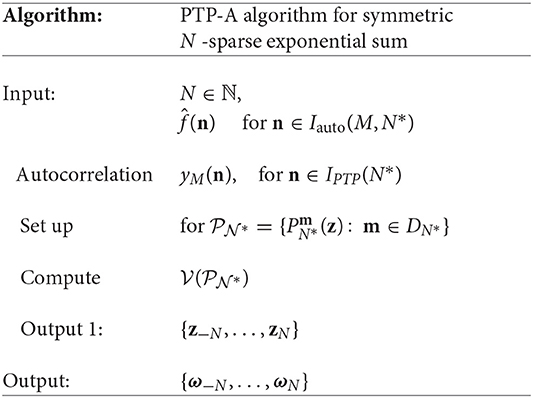
Using autocorrelation in the case of noisy data helps us to stabilize the result. Theorem 4.2.1 provides the following algorithm that we call PTP-A algorithm.

Lemma 4.2.1. Let $N^{*}=\frac{n(n+1)}{2}+i$, for n ∈ ℤ₊ and 0 ≤ i ≤ n, then, the set of samples $I_{\text{auto}}(M,N^{*})$ of $\widehat{f}$ required by the PTP-A algorithm with the window size M fulfills

$\begin{array}{l}\#I_{\text{auto}}(M,N^{*})\\ =\{\begin{array}{ll}4M^2+(4M-3)\sqrt{8(N^{*}-i)+1}-4i-4M+6N^{*}-2,& \text{if }i>0,\\ 4M^2+4(M-1)\sqrt{8N^{*}+1}-8M+6N^{*}+3,& \text{if }i=0.\end{array}\end{array}$

Proof. To investigate the number of samples of the N-sparse bivariate exponential sum $\widehat{f}$ that are needed for the PTP-A-algorithm, let us, first of all, analyze the structure of the autocorrelation sequence itself. For some fixed n ∈ ℤ² and given the size of the window M, an element of the autocorrelation sequence defined in (28)

$\begin{array}{l}{y}_M(\text{n})=\frac{1}{{\text{Ψ}}_M(0,0)}{\displaystyle \sum _{\text{k}\in {\mathbb{Z}}^2}}{H}_M(\text{k})\widehat{f}(\text{k})\frac{\widehat{f}(\text{k}+\text{n})+\widehat{f}(\text{k}-\text{n})}{2}\end{array}$

involves $\widehat{f}(\text{k}),\widehat{f}(\text{k}+\text{n})$, and $\widehat{f}(\text{k}-\text{n})$. On the one hand, this means that to compute one element y_M(n) we need all values of $\widehat{f}(\text{k})$, for $\text{k}=(k_1,k_2)\in {\mathbb{Z}}^2$ with ||k||_∞ < M, since H_M(k) = 0 if either |k₁| ≥ M or |k₂| ≥ M. We call the set of vectors k ∈ ℤ² that has the property ||k||_∞ < M with some fixed window size M a window sample set and denote it by $I_{\text{window}}(M)=\left\{\text{k}\in {\mathbb{Z}}_{+}^2:\left|\right|\text{k}|{|}_{\infty }<M\right\}$ (see Figure 4B). On the other hand, y_M(n) also requires values of $\widehat{f}(\text{k}+\text{n})$ and $\widehat{f}(\text{k}-\text{n})$, which of course supply some new samples of $\widehat{f}$ that have not yet appeared in I_window(M). However, these new sampling vectors are not more than the shifts of the window set in n and −n direction (see Figures 4B,C).

FIGURE 4

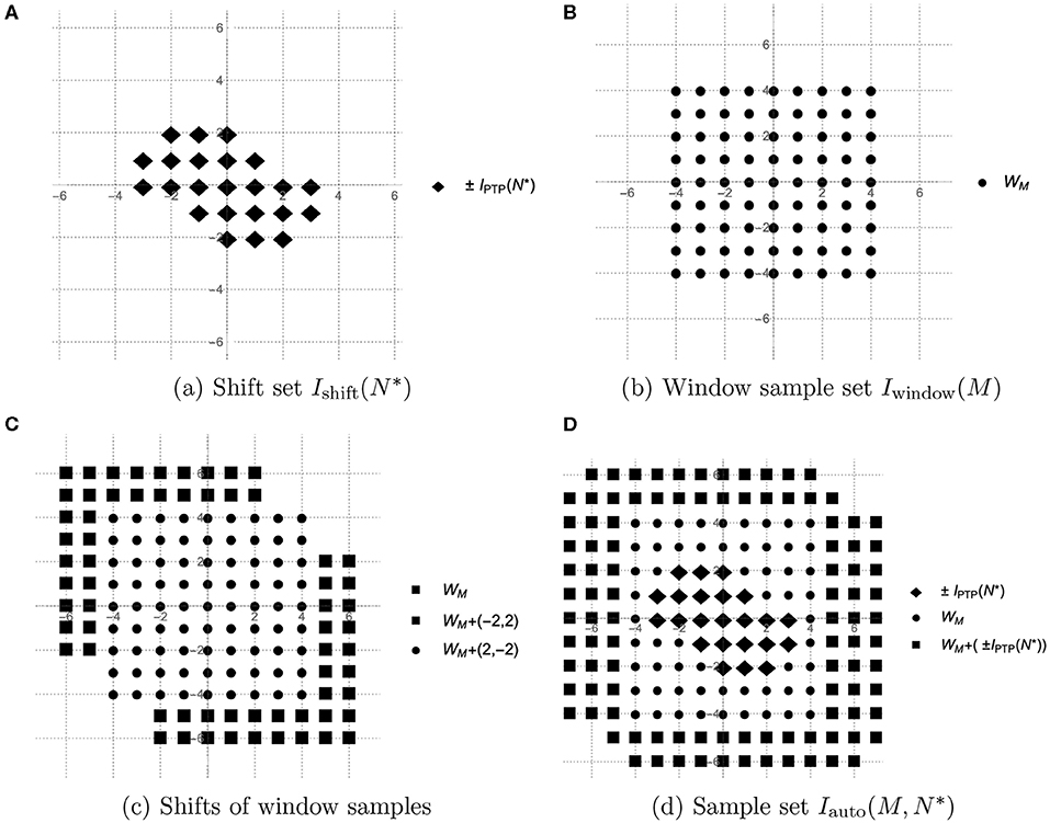
Figure 4. Sample sets of PTP-A algorithm. (A) Shift set $I_{\text{shift}}(N^{*})$, (B) Window sample set I_window(M), (C) Shifts of window samples, and (D) Sample set $I_{\text{auto}}(M,N^{*})$.

When applying the PTP-A algorithm, the structure of the Prony-type polynomials stays the same as for any N*-sparse exponential sum, the only difference is that we use y_M instead of $\widehat{f}$. This means that to build the Prony-type polynomials one needs to have the values of the autocorrelation sequence y_M(n) for all $\text{n}\in I_{PTP}(N^{*})=I_{N^{*}}\cup I_{N^{*}}^{+}$. Everything that is not changeable while computing y_M(n) for each $\text{n}\in I_{N^{*}}\cup I_{N^{*}}^{+}$ is the window sample set I_window(M) consisting of 2M + 1 samples of $\widehat{f}$. However, choosing different $\text{n}\in I_{N^{*}}\cup I_{N^{*}}^{+}$ causes different directions of shifting of I_window(M) and results in new samples of $\widehat{f}$ because computing y_M(n) requires $\widehat{f}(\text{k}+\text{n})$ and $\widehat{f}(\text{k}-\text{n})$. So, we need to move I_window(M) in n and in −n for all $\text{n}\in I_{N^{*}}\cup I_{N^{*}}^{+}$ to obtain the whole sample set for the PTP-A method. As it was mentioned in the poof of Lemma 3.2.1, the set $I_{N^{*}}$ has the properties $\forall \text{k}\in I_{N^{*}}:-\text{k}\in I_{N^{*}}\wedge (-\text{k}=\text{k}\iff \text{k}=(0,0))$ and some elements of $I_{N^{*}}^{+}$ are located also in $I_{N^{*}}$. This means that among the vectors $\left\{-\text{n}:\text{n}\in I_{N^{*}}\cup I_{N^{*}}^{+}\right\}$ the new ones used for shifting are only such that $\left\{-\text{n}:\text{n}\in I_{N^{*}}\backslash I_{N^{*}}^{+}\right\}$, and all other vectors have already occurred in $I_{N^{*}}\cup I_{N^{*}}^{+}$. Thus, all the shift vectors build the set

$I_{\text{shift}}(N^{*})=\left\{\text{n}\in I_{N^{*}}\cup I_{N^{*}}^{+}\right\}\cup \left\{-\text{n}:\text{n}\in I_{N^{*}}\backslash I_{N^{*}}^{+}\right\},$

which we call the shift set (see Figure 4A). Taking into account the above-mentioned properties of the shift set and some facts from Lemma 3.2.1, we can assert that

$\begin{array}{l}\#I_{\text{shift}}(N^{*})=\#I_{N^{*}}+2\#I_{N^{*}}^{+}\backslash I_{N^{*}}=2\#I_{N^{*}}^{\star }-1+2\#I_{N^{*}}^{+}\backslash I_{N^{*}}.\end{array}$

The set $I_{\text{shift}}(N^{*})$ almost builds the rectangular set

${{R}}_{N^{*}}=\{\begin{array}{llll}\text{m}=(m_1,m_2)\in {\mathbb{Z}}_{+}^2:& \left|m_1\right|\le n+1,& \left|m_2\right|\le n,& \text{if }i>0,\\ \text{m}=(m_1,m_2)\in {\mathbb{Z}}_{+}^2:& \left|m_1\right|\le n,& \left|m_2\right|\le n,& \text{if }i=0,\end{array}$

see Figure 4A, where n ∈ ℤ₊ and 1 ≤ i ≤ n follow from the representation $N^{*}=\frac{n(n+1)}{2}+i$. Clearly, the number of vectors that are in ${{R}}_{N^{*}}\backslash I_{\text{shift}}(N^{*})$ can be computed as $\#{{R}}_{N^{*}}-\#I_{\text{shift}}(N^{*})$.

Since we are shifting the rectangular window sample set I_window(M) using the vector n from the almost rectangular set $I_{\text{shift}}(N^{*})$, we get the set

$\begin{array}{l}{I}_{\text{auto}}(M,N^{*})=\left\{\text{k}\pm \text{n}:\text{k}\in I_{\text{window}}(M),\text{n}\in I_{N^{*}}\cup I_{N^{*}}^{+}\right\},\end{array}$

see Figure 4D, that also almost builds a rectangle

$\begin{array}{l}{{R}}_{N^{*},M}\\ =\{\begin{array}{llll}\text{m}=(m_1,m_2)\in {\mathbb{Z}}_{+}^2:& \left|m_1\right|\le M+n,& \left|m_2\right|\le M+n-1,& \text{if }i>0,\\ \text{m}=(m_1,m_2)\in {\mathbb{Z}}_{+}^2:& \left|m_1\right|\le M+n-1,& \left|m_2\right|\le M+n-1,& \text{if }i=0.\end{array}\end{array}$

The number of vectors that lack in I_auto to form the rectangle ${{R}}_{N^{*},M}$ is caused exactly by the absence of vectors $\text{n}\in {{R}}_{N^{*}}\backslash I_{\text{shift}}(N^{*})$, and is equal to $\#{{R}}_{N^{*}}-\#I_{\text{shift}}(N^{*})$. It follows

$\begin{array}{l}\#I_{\text{auto}}(M,N^{*})=\#{{R}}_{N^{*},M}-(\#{{R}}_{N^{*}}-\#I_{\text{shift}}(N^{*})).\end{array}$

Accordingly, the number of points in the rectangles are

${{R}}_{N^{*}}=\{\begin{array}{ll}(2(n+2)-1)(2(n+1)-1),& \text{if }i>0,\\ {(2(n+1)-1)}^2,& \text{if }i=0,\end{array}$

$\begin{array}{l}{{R}}_{N^{*},M}=\{\begin{array}{ll}(2(M+n+1)-1)(2(M+n)-1),& \text{if }i>0,\\ {(2(M+n)-1)}^2,& \text{if }i=0.\end{array}\end{array}$

Taking into account (20), (21) for i = 0, and (22), (23) when i > 0, and simplifying the corresponding expressions, we obtain

$\begin{array}{l}\#I_{\text{auto}}(M,N^{*})\\ =\{\begin{array}{ll}4(M+2n+1)(M-1)-3n^2-5n-2i+1,& \text{if }i>0,\\ 4(M+2n)(M-1)-(3n^2+3n-1),& \text{if }i=0\end{array}\end{array}$

and in terms of N* this equals

$\begin{array}{l}\#I_{\text{auto}}(M,N^{*})\\ =\{\begin{array}{ll}4M^2+(4M-3)\sqrt{8(N^{*}-i)+1}-4i-4M+6N^{*}-2,& \text{if }i>0,\\ 4M^2+4(M-1)\sqrt{8N^{*}+1}-8M+6N^{*}+3,& \text{if }i=0\end{array}\end{array}$

that finishes the proof□.

4.3. Autocorrelation Sequence and Exponential Sum Without Symmetry

As we have seen in the previous section, the PTP-A algorithm is applicable for symmetric exponential sums. In this subsection we propose a generalization of this method to non-symmetric exponential sums.

Let us consider the N-sparse bivariate exponential sum

$\begin{array}{l}f(\text{n})={\displaystyle \sum _{j=1}^N}{a}_{j}exp(-\text{i}\langle {\omega }_j,\text{n}\rangle )={\displaystyle \sum _{j=1}^N}{a}_j{\text{z}}_j^{\text{n}},\text{n}\in {\mathbb{Z}}^2,\end{array}$

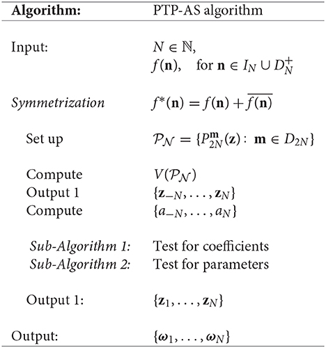
where N ∈ ℕ, a₁, a₂, …, a_N ∈ ℂ\{0} and ${\omega }_j=({\omega }_{j,1},{\omega }_{j,2})\in [0,2\pi ){}^2$ with ω_j ≠ ω_k for j ≠ k, and exp(−iω_j) = z_j, j, k = 1, …, N. Then, we symmetrize f by forming the real-valued sequence

$f^{*}(\text{n})=f(\text{n})+\overline{f(\text{n})},\text{n}\in {\mathbb{Z}}^2,$

which we call an assistant sequence. It is easy to see that the sequence f* is of symmetric structure (27), therefore all the statements described in the previous section hold for f*, and this allows us to apply the PTP-A algorithm to recover the parameters of f*. The problem here is that the set of parameters we get as output, obviously includes not only z₁, …, z_N but also ${\overline{\text{z}}}_1,\dots ,{\overline{\text{z}}}_N$. Therefore, we need to add a few steps more to the original PTP-A algorithm to distinguish the true parameters from the additional one. To this aim, let us, first of all, recover the coefficients of f*, i.e., a _{− N}, …, a_N. This can be done by solving the linear system of equations

$\begin{array}{r}\left(\begin{array}{cccc}1& 1& \cdots & 1\\ {\text{z}}_{-N}^{(l(1),r(1))}& {\text{z}}_{-(N-1)}^{(l(1),r(1))}& \cdots & {\text{z}}_N^{(l(1),r(1))}\\ ⋮& ⋮& ⋮& ⋮\\ {\text{z}}_{-N}^{(l(2N),r(2N))}& {\text{z}}_{-(N-1)}^{(l(2N),r(2N))}& \cdots & {\text{z}}_N^{(l(2N),r(2N))}\end{array}\right)\left(\begin{array}{c}{a}_{-N}\\ a_{-(N-1)}\\ ⋮\\ a_N\end{array}\right)\\ =\left(\begin{array}{c}{f}_{0,0}\\ f_{l(1),r(1)}\\ ⋮\\ f_{l(2N),r(2N)}\end{array}\right).\end{array}$

Having recovered the coefficients a _{− N}, …, a_N of the assistant sequence f*, we are interested in the exact coefficients of the initial exponential sum f. The coefficients we are looking for form one of the N-subsets of the set A = {a _{− N}, …, a_N}. So we need to analyze all subsets of set A that consist of N elements, where the order of elements is not important.

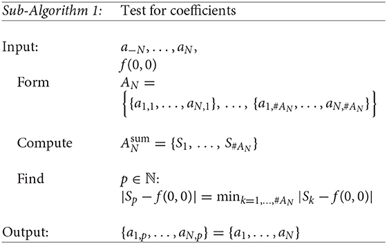
Let us denote by A_N the set of all N-subsets of set A. Since $\#A_N=\left(\frac{2N}{N}\right)$, we can represent the set A_N in the following way:

$A_N=\{\{a_{1,1},\dots ,a_{N,1}\},\dots ,\{a_{1,\#A_N},\dots ,a_{N,\#A_N}\}\}.$

It is obvious that the given sample f(0, 0) is just the sum of a₁, …, a_N. Therefore, we can use this information to find out which of these N-subsets of A is the correct set, or in other words, which consists of the initial coefficients. By computing for each N-subset the sum of its elements $S_k={\sum }_{i=1}^N{a}_i^k$ for k = 1, …, #A_N and finding the minimum among all the differences |S_k − f(0, 0)|, i.e., ${min}_{k=1,\dots ,\#A_N}|S_k-f(0,0)|$, we can determine the exact coefficients a₁, …, a_N. This method is described in the next sub-algorithm:

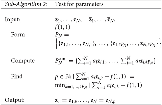
In order to find the exact parameters of the exponential sum f among z₁, …, z_N, but also ${\overline{\text{z}}}_1,\dots ,{\overline{\text{z}}}_N$, we describe a similar procedure. In this case, we consider the set of all N-subsets of the set $P=\left\{{\text{z}}_1,\dots ,{\text{z}}_N,{\overline{\text{z}}}_1,\dots ,{\overline{\text{z}}}_N\right\}$. However in this case the order of elements is important. We denote this set by

$\begin{array}{ll}{P}_N=\{\{{\text{z}}_{1,1},\dots ,{\text{z}}_{N,1}\},\dots ,\{{\text{z}}_{1,\#P_N},\dots ,{\text{z}}_{N,\#P_N}\}\},& (30)\end{array}$

where $\#P_N=\frac{(2N)!}{N!}$. To distinguish here between the true and additional parameters we use the value f(1, 1) and for k = 1, …, #P_N we consider the differences between ${\sum }_{i=1}^N{a}_i{\text{z}}_{i,k}$ and f(1, 1). Then, one of these N-subsets, for which the difference $|{\sum }_{i=1}^N{a}_i{\text{z}}_{i,k}-f(1,1)|$ is minimal, forms the set of the exact parameters of the exponential sum f. Thus, we have got the second sub-algorithm:

In general, we have the algorithm to find the frequency vectors of the exponential sum f :

5. Numerical Computations

In this section we present some numerical results related to the stability of the suggested methods in case of noise corruption.

We have implemented the PTP, PTP-A, and PTP-AS algorithms in Mathematica with a working precision of 50 digits. For numerical computation we use the following numerical method, which we call an intersection method. For the intersection method we use three (for example the first three) Prony-type polynomials $P_N^{\text{m}}$, $\text{m}\in D_N^{†}:=\left\{(l(j),r(j)):j=N,\dots ,N+2\right\}$, for an exponential sum f independently of a number of parameters N in the sum. Then, having found common zeros of the first and the second, and of the second and the third polynomial, we compute the intersection of these two zero sets under the condition that at least one digit after the comma coincides. To avoid the case when the intersection set consists of too many parameters, at the end of the intersection method we perform an additional test for the common zeros asking for N elements z_j = (z_{1, j}, z_{2, j}) that have components with an absolute value between 0.99 and 1.01, namely 0.99 ≤ |z_{i, j}| ≤ 1.01, j = 1, …, N and i = 1, 2.

Experiment 1. For the first experiment we have considered the 5-sparse exponential sum

$\begin{array}{l}f(\text{n})={\displaystyle \sum _{j=1}^5}{a}_{j}exp(-\text{i}\langle {\omega }_j,\text{n}\rangle )+\epsilon (\text{n}),\text{n}\in {\mathbb{Z}}^2,\end{array}$

with complex coefficients a₁, a₂, …, a₅ ∈ ℂ\{0}, pairwise distinct frequency vectors ${\omega }_j=({\omega }_{j,1},{\omega }_{j,2})\in [0,2\pi ){}^2,$ j = 1, …, 5, and additive noise ε(n). The noise ε(n) is also complex-valued and is of the form ε(n) = ϵe^iφ with a random absolute value ϵ uniformly distributed in [1 × 10^−η, 9 × 10^−η], η = 2, …, 30 and a random angle φ uniformly distributed in [0, 2π).

Using the data of one hundred randomly generated collections of coefficients and the separated frequency vectors

$\{\left\{a_1,a_2,a_3,a_4,a_5\right\},\left\{{\omega }_1,{\omega }_2,{\omega }_3,{\omega }_4,{\omega }_5\right\}\},$

we have tested on these data three algorithms, namely, the method of the minimal number of samples (MNS) of Cuyt and Wen-Shin [4] with the sampling direction Δ = (1, 0) and the shift vector δ = (0, 1), the PTP algorithm and the PTP-AS algorithm with window size M = 50 and M = 100 (PTP-AS-50 and PTP-AS-100, respectively). In our numerical experiments we consider as an error the ℓ₂-norm,

$\Delta {\omega }_j=\left|\right|{\omega }_j-{\tilde{\omega }}_j|{|}_2,j=1,\dots ,5,$

where ${\tilde{\omega }}_j$, j = 1, …, 5, are frequency vectors recovered due to one of the considered algorithms. Afterwards, we consider the maximal deviation $\Delta =\underset{j=1,\dots ,5}{max}(\Delta {\omega }_j)$ per trail, and for each level of noise η = 2, …, 30, we compute the average of the maximal deviations over 100 settings.

The obtained numerical results of Experiment 1 are shown in Tables 1, 2 and Figure 5.

TABLE 1

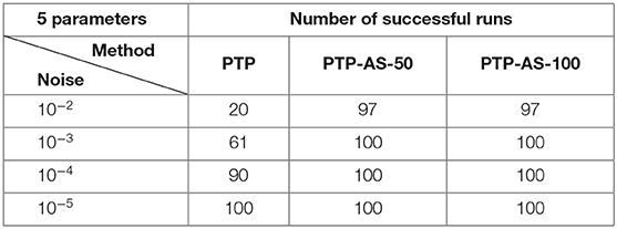
Table 1. Results of Experiment 1.

TABLE 2

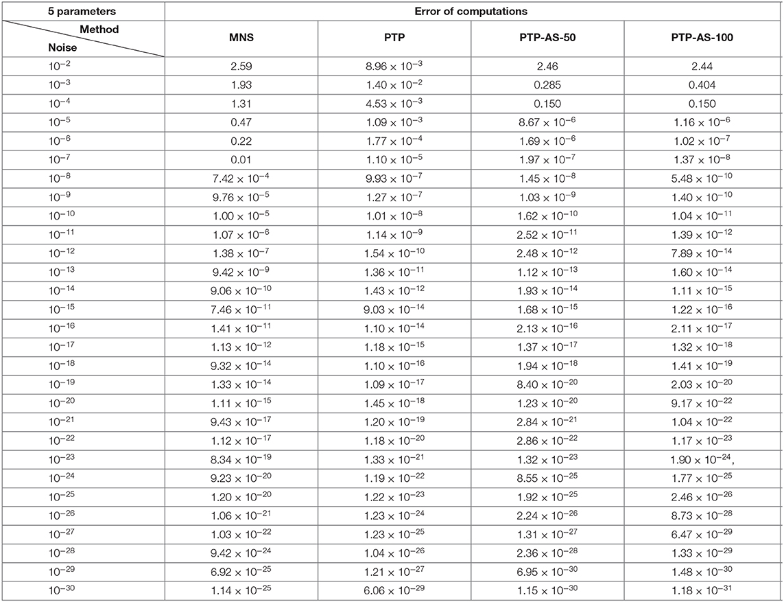
Table 2. Results of Experiment 1.

FIGURE 5

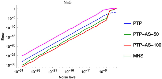
Figure 5. Results of Experiment 1.

Experiment 2. For the second experiment we have considered the symmetric 6-sparse exponential sum

$\begin{array}{l}f(\text{n})={\displaystyle \sum _{j=-6}^6}{a}_{j}exp(-\text{i}\langle {\omega }_j,\text{n}\rangle )+\epsilon (\text{n}),\text{n}\in {\mathbb{Z}}^2,\end{array}$

with complex coefficients a₁, a₂, …, a₆ ∈ ℂ\{0}, pairwise distinct frequency vectors ${\omega }_j=({\omega }_{j,1},{\omega }_{j,2})\in [0,\pi ){}^2,$ j = 1, …, 6, and additive noise ε(n). As in the previous case the noise ε(n) is also complex-valued and is of the form ε(n) = ϵe^iφ with a random absolut value ϵ uniformly distributed in [1 × 10^−η, 9 × 10^−η], η = 2, …, 30 and a random angle φ uniformly distributed in [0, 2π).

Here, we have used the data of one hundred randomly generated collections of coefficients and the well separated frequency vectors

$\{\left\{a_1,a_2,a_3,a_4,a_5,a_6\right\},\left\{{\omega }_1,{\omega }_2,{\omega }_3,{\omega }_4,{\omega }_5,{\omega }_6\right\}\}$

with the properties $a_{-j}=\overline{a_j}$ and ω _{− j} = −ω_j for all j = 1, …, 6. We have tested on these data three algorithms, namely the same MNS method with the sampling direction Δ = (1, 0) and the shift vector δ = (0, 1) (see [4]), the PTP algorithm and the PTP-A algorithm with window size M = 50 and M = 100 (PTP-A-50 and PTP-A-100, respectively). In our numerical experiments we consider the ℓ₂-norm error, $\Delta {\omega }_j=\left|\right|{\omega }_j-{\tilde{\omega }}_j|{|}_2,j=-6,\dots ,6,$ and compute the average of the maximal deviations $\Delta ={max}_{j=-6,\dots ,6}(\Delta {\omega }_j)$ over 100 settings. The numerical results of Experiment 2 are shown in Tables 3, 4 and Figure 6.

TABLE 3

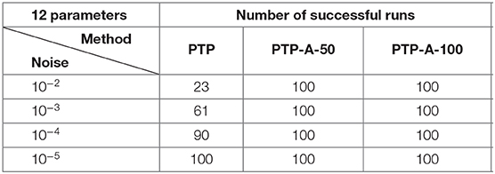
Table 3. Results of Experiment 2.

TABLE 4

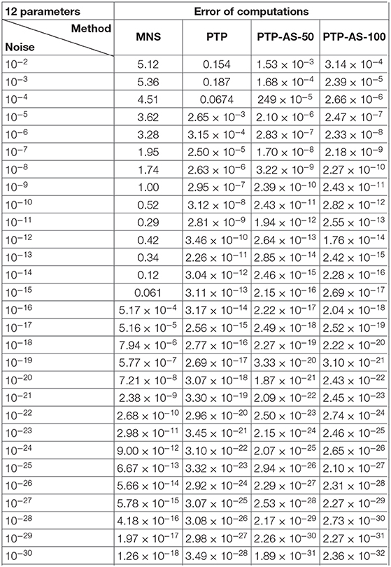
Table 4. Results of Experiment 2.

FIGURE 6

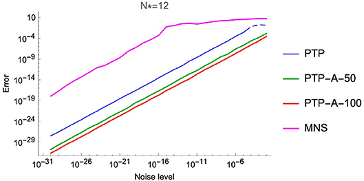
Figure 6. Results of Experiment 2.

As numerical computations show, the methods of the PTP type stay more stable in the case of noise corruption. Moreover, the PTP-A algorithm has a good performance, even if the level of noise is of the order 10⁻². Of course, in this case we need to ask for more samples (see Lemma 4.2.1) of the exponential sum.

Data Availability Statement

All datasets generated and analyzed for this study are included in the article/supplementary material.

Author Contributions

All authors listed have made a substantial, direct and intellectual contribution to the work, and approved it for publication.

Funding

This research was supported by the DAAD Research Grant for Doctoral Candidates and Young Academics and Scientists 2017/18 (57299291) and the Horizon 2020 project AMMODIT—Grant Number MSCA-RISE 645672. Besides, we acknowledge support by the German Research Foundation and the Open Access Publication Funds of the Technische Universität Braunschweig.

Conflict of Interest

The authors declare that the research was conducted in the absence of any commercial or financial relationships that could be construed as a potential conflict of interest.

Acknowledgments

First of all, the authors would like to thank Prof. Stefan Kunis for his valuable comments and remarks to improve this paper. The authors are most grateful to Frederic Schoppert for his numerical computations and the discussions about the number of samples required by the method of Prony-type polynomials. Furthermore, the authors are thankful to Prof. Anne Frühbis-Krüger for fruitful discussions.

References

1. Kunis S, Peter T, Römer T, von der Ohe U. A multivariate generalization of Prony's method. Linear Algebra Appl. (2016) 490:31–47. doi: 10.1016/j.laa.2015.10.023

CrossRef Full Text | Google Scholar

2. Cuyt A, Tsai M, Verhoye M, Wen-Shin L. Faint and clustered components in exponential analysis. Appl Math Comput. (2018) 327:93–103. doi: 10.1016/j.amc.2017.11.007

CrossRef Full Text | Google Scholar

3. Diederichs B, Iske A. Parameter estimation for bivariate exponential sums. In: 2015 International Conference on Sampling Theory and Applications (SampTA) (2015). p. 493–97.

Google Scholar

4. Cuyt A, Wen-Shin L. Multivariate exponential analysis from the minimal number of samples. Adv Comput Math. (2016) 44:987–1002. doi: 10.1007/s10444-017-9570-8

CrossRef Full Text | Google Scholar

5. Filbir F, Mhaskar HN, Prestin J. On the problem of parameter estimation in exponential sums. Constr Approx. (2012) 35:323–43.

Google Scholar

6. Teplan M. Fundamentals of EEG measurement. Measure Sci Rev. (2002) 2:1–11.

Google Scholar

7. Sanei S, Chambers JA. EEG Signal Processing. John Wiley and Sons (2013).

Google Scholar

8. Webster JG, Eren H, editors. Measurement, Instrumentation, and Sensors Handbook: Electromagnetic, Optical, Radiation, Chemical, and Biomedical Measurement. 2nd Edition. Boca Raton, FL: CRC-Press (2014).

Google Scholar

9. Semmler G, Wegert E. Finite Blaschke products with prescribed critical points, Stieltjes polynomials, and moment problems. Anal Math Phys. (2019) 9:221–49. doi: 10.1007/s13324-017-0193-5

CrossRef Full Text | Google Scholar

10. de Prony BGR. Essai expérimental et analytique sur les lois de la dilatabilité des fluides élastiques et sur celles de la force expansive de la vapeur de l'eau et de la vapeur de l'alcool á différentes températures. J Éc. Polytech. (1795) 1:24–76.

Google Scholar

11. Schmidt R. Multiple emitter location and signal parameter estimation. IEEE Trans Antennas Propagat. (1986) 34:276–80.

Google Scholar

12. Roy R, Kailath T. ESPRIT-estimation of signal parameters via rotational invariance techniques. IEEE Trans Acoust Speech Signal Process. (1989) 37:984–95.

Google Scholar

13. Hua Y. Estimating two-dimensional frequencies by matrix enhancement and matrix pencil. In: International Conference on Acoustics, Speech, and Signal Processing (1992). p. 2267–80.

Google Scholar

14. Plonka G, Wischerhoff M. How many Fourier samples are needed for real function reconstruction? J Appl Math Comput. (2013) 42 :117–37. doi: 10.1007/s12190-012-0624-2

CrossRef Full Text | Google Scholar

15. Potts D, Tasche M. Parameter estimation for multivariate exponential sums. Electron Trans Numer Anal. (2013) 40:204–24. doi: 10.1007/978-3-319-16721-3

CrossRef Full Text

16. Sauer T. Prony's method in several variables: Symbolic solutions by universal interpolation. J Symb Comput. (2018) 84:95–112. doi: 10.1016/j.jsc.2017.03.006

CrossRef Full Text | Google Scholar

17. Josz C, Lasserre JB, Mourrain B. Sparse polynomial interpolation: sparse recovery, super-resolution, or Prony? Adv Comput Math. (2019) 45:1401–37. doi: 10.1007/s10444-019-09672-2

CrossRef Full Text | Google Scholar

18. Pan KC, Saff EB. Asymptotics for zeros of Szegő polynomials associated with trigonometric polynomial signals. J Approx Theory. (1992) 71:239–51.

Google Scholar

19. Cox D, Little J, O'shea D. Ideals, Varieties, and Algorithms. Vol. 3. New York, NY: Springer (2007).

20. Dunkl CF, Xu Y. Orthogonal Polynomials of Several Variables. 2nd Edition. Cambridge University Press (2014).

Google Scholar

21. Cantor G. Ein beitrag zur mannigfaltigkeitslehre. J Reine Angew Math. (1878) 84:242–58.

Google Scholar

22. Sturmfels B. WHAT IS…a Gröbner basis? Not AMS. (2005) 52:1199.

Google Scholar

23. Kunis S, Potts D. Stability results for scattered data interpolation by trigonometric polynomials. J Sci Comput. (2007) 29:1403–19. doi: 10.1137/060665075

CrossRef Full Text | Google Scholar