CARMA Approximations and Estimation

1. Introduction

Continuous-time autoregressive moving-average processes, CARMA in short, represent the continuous-time version of the well-known ARMA models. Because of their linear structure, they are convenient for modeling empirical data, hence they find application in several fields, particularly in finance. Indeed, with a Lévy process as a driver for the noise, one obtains a rich class of possibly heavy-tailed continuous-time stationary processes, and such heavy tails are frequently observed in finance [1]. In Barndorff-Nielsen and Shepard [2], for example, a Lévy-driven Ornstein-Uhlenbeck process (corresponding to a CAR(1)) is employed in a stochastic volatility model, and [3] extend the idea to a wider class of Lévy-driven CARMA processes with non-negative kernel, allowing for non-negative, heavy-tailed processes with a larger range of autocovariance functions.

In view of financial applications, Brockwell et al. [4] derive efficient estimates for the parameters of a non-negative Lévy-driven CAR(1) process, and Brockwell et al. [5] generalize the technique to higher-order CARMA processes with a non-negative kernel. In Benth et al. [6] and Benth and Benth [7], the authors exploit the link between discrete-time ARMA and continuous-time ARMA to model the observed processes in a continuous manner, starting from discrete-time observations-based estimates, in the context of energy markets and weather derivatives. It is also worth mentioning that CARMA processes allow us to construct a wide range of long-memory processes, as shown, e.g., in Marquardt [8] and Marquardt and James [9].

Among the several financial applications, in Paschke and Prokopczuk [10, 11] a CARMA process is employed for the long-term equilibrium component in the two-factors spot price model introduced by Schwartz and Smith [12] (which uses an Ornstein-Uhlenbeck process), while Benth and Koekebakker [13] use a CARMA process for the short-term factor instead. In Benth et al. [14] and García et al. [15], a CARMA process models the spot price in the electricity market, while in Benth et al. [6] and Benth and Benth [7] it models weather variables, such as temperature and wind speed. Finally, Andresen et al. [16] apply CARMA processes to interest rates modeling and [17] to the dynamics of regional ocean freight rates.

Formally, CARMA(p, q) processes are compactly defined through a stochastic differential equation (SDE) involving q + 1 derivatives of the Lévy process driving the noise, despite the latter having in general no differentiable paths. Numerical schemes, such as the Euler scheme, are also applied both for simulations and estimation of CARMA processes. These schemes approximate derivatives with discrete increments with respect to a time step Δ, and their convergence for Δ approaching zero is indeed a well-studied topic. However, this opens up for a discrepancy since it is not mathematically clear what happens when the time step approaches zero, as, in general, the derivatives of a Lévy process are not well-defined.

We give a mathematical justification for the representation via SDE of a CARMA process, and, consequently, for the discrete approximations used for simulating and estimating the continuous-time dynamics of CARMA processes. This is done by replacing the Lèvy process L driving the noise with a process smooth enough so that the SDE makes mathematical sense. For ε > 0 we construct a continuously differentiable function L_ε, which converges in the L² sense to the original Lévy process in the space [0, T] × Ω, for T < +∞. More precisely, the process L_ε is constructed via stochastic convolution of L with a smooth sequence of functions {ϕ_ε}_ε>0 depending on the convolution parameter ε > 0 and with first derivative converging to the delta-Dirac function when ε approaches zero. We show a rate of convergence of order 1.

For the L_ε continuous differentiable, the framework developed solves the differentiability issue for CAR(p) processes in which no more than the first derivative of the driving noise process is required. We can, however, make use of the result in Brockwell et al. [5, Proposition 2]. This states that, under some conditions on the coefficients of the SDE, a CARMA(p, q) process can be decomposed into a sum of p dependent CAR(1) processes. The approach can then be extended to CARMA(p, q) processes of every order q ≥ 0 by considering p different approximations based on the continuous differentiable L_ε and taking their sum. This justifies an L_ε-only continuous differentiable, as the general case q ≥ 0 is still covered.

We thus replace the Lèvy process L with L_ε in the SDE defining the CARMA process X. This gives a different SDE, which depends on ε, whose solution is the new process X_ε. We show that X_ε converges to X in L²([0, T] × Ω) and that the convergence is of order 2.

The ε-approximation of the Lévy process justifies the use of an Euler scheme for every time step Δ. We present a possible approach for simulating L_ε starting from a simulated path of the Lèvy process L and then X_ε starting from L_ε. This, for a fixed time interval Δ, gives a new noise process $L_{\epsilon }^{\Delta }$ and a third process $X_{\epsilon }^{\Delta }$. We show a rate of convergence for both $L_{\epsilon }^{\Delta }$ and $X_{\epsilon }^{\Delta }$ proportional to Δ² and inversely so to ε. This highlights that the two parameters Δ and ε must be chosen in a way to get accurate simulations and prevent them from exploding.

We finally consider a possible Euler scheme approach for estimating the CARMA dynamics starting from the simulated time series. It is worth mentioning that the process L_ε is not a Lèvy process. Due to the convolution operator, it indeed fails on the crucial property of independent increments. We show in particular that the increments depend on the ratio $\frac{\Delta }{\epsilon }$, and, as this ratio becomes smaller, the increments become more dependent on each other. This has a negative drawback when it comes to estimation. We find indeed that the Euler scheme recovers the true dynamics of the CARMA process only if ε is smaller than Δ.

All the results are deeply investigated and are also confirmed by numerical experiments. In particular, we consider two different Lèvy processes, a Brownian motion and a normal inverse Gaussian (NIG) process, and CARMA processes of two different orders, a Gaussian CAR(1) and a Gaussian CARMA(3, 2). Crucial to all the numerical simulations is the convolution property of both the Gaussian and the NIG distribution function, which allows us to compare path-wise different time grids by simulating only one path of the Lèvy process.

Since CARMA processes have significant application within finance, from the modeling of the electricity spot price to the modeling of wind speed and temperature, with the present study, we justify its mathematical formulation and application in a rigorous way. Moreover, this may open for further applications in the context of sensitivity analysis with respect to paths of the driving noise process. Indeed, since the new process L_ε admits derivatives, one could potentially analyze the sensitivity of the CARMA process, and hence of the variable of interest (e.g., the spot price), with respect to the Lévy noise in a path-wise sense. It might also be that when observing a signal, the driving-noise process is more regular than, e.g., a Brownian motion. This might then be modeled by the regular process here introduced and studied.

The rest of the paper is organized as follows. In section 2 we construct the approximating process L_ε by stochastic convolution, and we study the rate of convergence. In section 3 we introduce CARMA processes and their spectral representation. We then show the convergence of the new process X_ε to the original CARMA process, and we briefly recover the general case q > 0. In section 4 we study an Euler scheme to simulate the process X_ε starting from the simulations of L_ε, and then to calibrate the parameters of the CARMA dynamics starting from the discrete time series. Appendix A in Supplementary Material contains the proofs of the main results.

2. Construction and Convergence Results

Let $(\Omega ,{F},\mathbb{P})$ be a probability space. We consider a one-dimensional Lèvy process L, which we assume to be a square-integrable martingale with characteristic triplet (κ, Σ, ν), ν being the Lévy measure. From Cont and Tankov [18, Proposition 3.13], for every t > 0 the variance of L(t) is of the form

$\begin{array}{ll}\text{Var }\left(L(t)\right)=t{\sigma }^2\text{ with }{\sigma }^2:=\Sigma +{\displaystyle {\int }_{-\infty }^{\infty }}{x}^2\nu (dx).& (2.1)\end{array}$

Moreover, from Cont and Tankov [18, Proposition 3.18], we also know that L is a martingale if, and only if,

$\begin{array}{ll}{\displaystyle {\int }_{|x|\ge 1}}|x|\nu (dx)<\infty \text{ and }\kappa +{\displaystyle {\int }_{|x|\ge 1}}x\nu (dx)=0.& (2.2)\end{array}$

We now consider a sequence of measurable functions {ϕ_ε}_ε>0 :[0, T] → ℝ such that, for every ε > 0, ϕ_ε is twice continuously differentiable on the interval [0, T] and ϕ_ε(0) = 0. We then construct the process {L_ε(t), t ≥ 0} by stochastic convolution of the Lévy process L with ϕ_ε:

$\begin{array}{ll}{L}_{\epsilon }(t):={\displaystyle {\int }_0^t}{\varphi }_{\epsilon }(t-s)dL(s).& (2.3)\end{array}$

L_ε is well-defined in [0, T] for every T ∈ ]0, +∞[, and, in particular, the condition ϕ_ε(0) = 0 is used to prove the following result, where the symbol * denotes the convolution operator.

Lemma 2.1. The process {L_ε(t), t ≥ 0} in Equation (2.3) can be expressed by

$\begin{array}{ll}{L}_{\epsilon }(t)=\left({\varphi }_{\epsilon }^{\prime }*L\right)(t){|}_{\left[0,t\right]}={\displaystyle {\int }_0^t}{\varphi }_{\epsilon }^{\prime }(t-s)L(s)ds.& (2.4)\end{array}$

Proof: See Appendix A.1 in Supplementary Material.

For ${\psi }_{\epsilon }(x):={\varphi }_{\epsilon }^{\prime }(x)$, since ϕ_ε(0) = 0, we write that ${\varphi }_{\epsilon }(t)={\int }_0^t{\psi }_{\epsilon }(u)du$ so that ϕ_ε is twice continuously differentiable for any continuously differentiable ψ_ε. We introduce the function $\psi (x):=\frac{2}{\sqrt{2\pi }}\text{exp}\left\{-\frac{1}{2}{x}^2\right\}$, and for every ε > 0 we define

$\begin{array}{ll}{\psi }_{\epsilon }(x):=\frac{1}{\epsilon }\psi \left(\frac{x}{\epsilon }\right)=\frac{2}{\sqrt{2\pi }\epsilon }\text{exp}\left\{-\frac{x^2}{2{\epsilon }^2}\right\}.& (2.5)\end{array}$

Let us notice that ${\int }_{ℝ}\psi (x)dx={\int }_{ℝ}{\psi }_{\epsilon }(x)dx=2$, while the total area of the mollifier function usually equals 1. However, we construct the process {L_ε(t), t ≥ 0} by stochastic convolution restricted to the interval [0, t], and, denoting by Φ the standard Gaussian cumulative distribution function, the area of ψ_ε restricted to [0, t] is

$\begin{array}{ll}\left({\varphi }_{\epsilon }(t)=\right){\displaystyle {\int }_0^t}{\psi }_{\epsilon }(x)dx=2\left(\Phi \left(\frac{t}{\epsilon }\right)-\frac{1}{2}\right){\displaystyle \underset{\text{}}{\overset{\epsilon \downarrow 0}{\to }}}1,& (2.6)\end{array}$

so that the unitary total integral property for ψ_ε is preserved in the limit.

By differentiating Equation (2.4) with respect to t, according to the Leibniz rule, we get

$\begin{array}{ll}{L}_{\epsilon }^{\prime }(t)={\varphi }_{\epsilon }^{\prime }(0)L(t)+{\displaystyle {\int }_0^t}{\varphi }_{\epsilon }^{″}(t-s)L(s)ds.& (2.7)\end{array}$

This shows that $L_{\epsilon }\in {{C}}^1([0,T])$, though $L_{\epsilon }\notin {{C}}^n([0,T])$ for any n > 1, because of the term L(t) which is not differentiable, unless ${\varphi }_{\epsilon }^{\prime }(0)={\psi }_{\epsilon }(0)=0$, which is not our case. Hence, we start with the Lévy process L, which is not differentiable, and we end up with L_ε, which is continuously differentiable. For a CARMA(p, q) process, we need $L_{\epsilon }\in {{C}}^{q+1}([0,T])$. From Equation (2.7), this means to have ${\varphi }_{\epsilon }^{(m)}(0)=0$ for every 0 ≤ m ≤ q + 1, ${\varphi }_{\epsilon }^{(m)}$ being the m-th derivative of ϕ_ε. However, for our particular choice of the convolution function ψ_ε, these conditions of null derivatives in zero are not satisfied. Another possible choice would have been, for example, to take a sequence of gamma densities with scale parameter θ_ε converging to 0 as ε converges to 0 and shape parameter k > 0, such as $d_{\epsilon }(t)=\frac{1}{\Gamma (k){\theta }_{\epsilon }^k}{t}^{k-1}{e}^{-\frac{t}{{\theta }_{\epsilon }}}.$ For k ≥ q + 1, the first q derivatives of d_ε are indeed null in t = 0.

With L_ε constructed above, we thus address the differentiability issue in the stochastic differential equation defining the CARMA process only for q = 0, namely when the process is a CAR(p). However, Brockwell et al. [5, Proposition 2] shows that, under some conditions, we can express a CARMA(p, q) process as the sum of p dependent and possibly complex-valued CAR(1) processes. The idea is then to construct the ε-approximation with L_ε in Equation (2.3) for each of the p processes of CAR(1)-type and obtain the ε-CARMA(p, q) process by summing them up. We can thus deal with q > 0, but it must be done separately. With the gamma densities mentioned above, for example, the special treatment for q > 0 would not be necessary. However, we started this analysis from CAR(p) processes, and in this setting the scaled Gaussian densities ψ_ε make the job. We shall analyze the case q > 0 in section 3.2.

A first important fact about L_ε in Equation (2.3) is that the convolution operation does not preserve the properties of the Lévy process L.

Proposition 2.2. The process {L_ε(t), t ≥ 0} is not a Lévy process.

Proof: See Appendix A.2 in Supplementary Material.

By Proposition 2.2, for L = B, a Brownian motion, the approximated process B_ε is no longer a Brownian motion. We can, however, show that the distribution of B is preserved.

Lemma 2.3. For every ε > 0, the process {B_ε(t), t ≥ 0} has Gaussian distribution with zero mean and variance

$\begin{array}{l}Var(B_{\epsilon }(t))={\displaystyle {\int }_0^t}{\varphi }_{\epsilon }^2(s)ds\\ =t+4t\Phi \left(\frac{t}{\epsilon }\right)\left(\Phi \left(\frac{t}{\epsilon }\right)-1\right)+\\ +4\epsilon \left(2\phi \left(\frac{t}{\epsilon }\right)\Phi \left(\frac{t}{\epsilon }\right)-\frac{1}{\sqrt{2}\pi }\left(\Phi \left(\frac{\sqrt{2}t}{\epsilon }\right)-\frac{1}{2}\right)-\phi \left(\frac{t}{\epsilon }\right)\right).\end{array}$

Proof: B_ε is defined in Equation (2.3) as the stochastic integral of ϕ_ε with respect to the Brownian motion B. Then B_ε has Gaussian distribution with zero mean and variance ${\int }_0^t{\varphi }_{\epsilon }^2(s)ds$, which can be explicitly calculated.□

Let us point out that Lemma 2.3 is valid for every choice of the functions {ϕ_ε}_ε>0, with the obvious modification for the variance formula ${\int }_0^t{\varphi }_{\epsilon }^2(s)ds$. Moreover, from Lemma 2.3, we get that ${\text{lim}}_{\epsilon \downarrow 0}\text{Var}(B_{\epsilon }(t))=t$, as one would expect. Figure 1 shows indeed the typical bell-shape for a Gaussian distribution. We sampled the process B_ε at time t = 1 for 5, 000 times and different values of ε. The empirical (black line) and the theoretical (red line) distributions (according to Lemma 2.3) are also shown. For ε = 1, there is a certain discrepancy between empirical and theoretical distributions, which may be due to the fact that for big values of ε the increments of B_ε are more dependent from each other than for smaller values of ε. The same phenomena will be encountered in section 4.3.

FIGURE 1

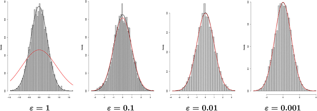
Figure 1. Histograms of B_ε(t) for t = 1 after 5, 000 simulations with Δ^true = 2⁻¹⁰ (n = 1, 024 points) and different ε's. Together, we have empirical (black line) and theoretical distribution (red line).

2.1. Convergence of the Lévy Approximation

We prove now the convergence of the process L_ε to the Lévy process L.

Theorem 2.4. The process {L_ε(t), t ≥ 0} converges to {L(t), t ≥ 0} in L²([0, T] × Ω).

Proof: See Appendix A.3 in Supplementary Material. The proof is based on some results from Benth et al. [19, Appendix A].

Figure 2 shows graphically the convergence stated in Theorem 2.4 for a Brownian motion and for a normal inverse Gaussian process with parameters (α, β, δ, μ) = (1, 0, Δ^true, 0), Δ^true being the time step used in the Euler discretization (see section 4). As ε decreases, the error between L_ε and L decreases. Even with a large ε (ε = 1), the process L_ε is able to capture the shape of L. It seems however to be slightly shifted to the right.

FIGURE 2

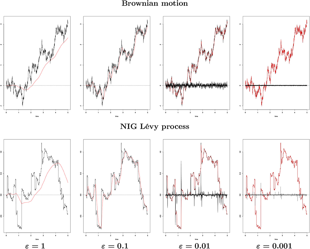
Figure 2. {L(t), 0 ≤ t ≤ 5} (black line) against {L_ε(t), 0 ≤ t ≤ 5} (red line) for different ε's generated from a single path with Δ^true = 2⁻¹⁰ (n = 5, 120 points) for a Brownian motion and a NIG process with parameters (α, β, δ, μ) = (1, 0, Δ^true, 0). The black bar lines in the four rightmost images represent the difference between L and L_ε.

We compute explicitly the squared error between L_ε and L at the terminal point t = T.

Lemma 2.5. For every ε > 0 and T < +∞, the squared error between L_ε and L is given by

$\begin{array}{l}𝔼\left[{\left(L_{\epsilon }(T)-L(T)\right)}^2\right]=4{\sigma }^{2}T{\left(\Phi \left(\frac{T}{\epsilon }\right)-1\right)}^2+\\ +4{\sigma }^2\epsilon (\frac{1}{\sqrt{2\pi }}+2\phi \left(\frac{T}{\epsilon }\right)\left(\Phi \left(\frac{T}{\epsilon }\right)-1\right)+\\ -\frac{1}{\sqrt{\pi }}\left(\Phi \left(\frac{\sqrt{2}T}{\epsilon }\right)-\frac{1}{2}\right)),\end{array}$

for σ² in Equation (2.1) and φ and Φ respectively the density and the cumulative distribution functions of a standard Gaussian random variable.

Proof: The proof applies the integration by parts formula several times.□

The following lemma concerning the cumulative Gaussian distribution function Φ is useful.

Lemma 2.6. The function Φ can be expanded by integration by parts into the series

$\begin{array}{ll}\Phi (x)=\frac{1}{2}+\frac{e^{-x^2/2}}{\sqrt{2\pi }}\left(x+{\displaystyle \sum _{n=1}^{\infty }}\frac{x^{2n+1}}{(2n+1)!!}\right),& (2.8)\end{array}$

!! denoting the double factorial. Moreover, for large x, the asymptotic expansion is also valid

$\begin{array}{ll}\Phi (x)=1-\frac{e^{-x^2/2}}{x\sqrt{2\pi }}\left(1+{\displaystyle \sum _{n=1}^{\infty }}{(-1)}^n\frac{(2n-1)!!}{x^{2n}}\right).& (2.9)\end{array}$

We now use the expansion (2.8) to calculate the rate of convergence of L_ε to the Lévy process L, starting from Lemma 2.5. The expansion (2.9) will be used further in the paper.

Proposition 2.7. For every ε > 0 and T < +∞, there exists a constant K₁ > 0 such that

$\begin{array}{l}𝔼\left[{\left(L_{\epsilon }(T)-L(T)\right)}^2\right]\le K_1\epsilon +O\left({\epsilon }^4\right).\end{array}$

Proof: See Appendix A.4 in Supplementary Material.

Similarly to Lemma 2.3, the rate of convergence found in Proposition 2.7 can be calculated explicitly for every choice of the functions {ϕ_ε}_ε>0, possibly obtaining a different order. The L² norm of the approximation error studied in Proposition 2.7 as a function of ε is in Figure 3A for the Brownian motion and in Figure 3B for the NIG Lévy process. In the next section we shall introduce CARMA processes in a more rigorous way and study their ε-approximation.

FIGURE 3

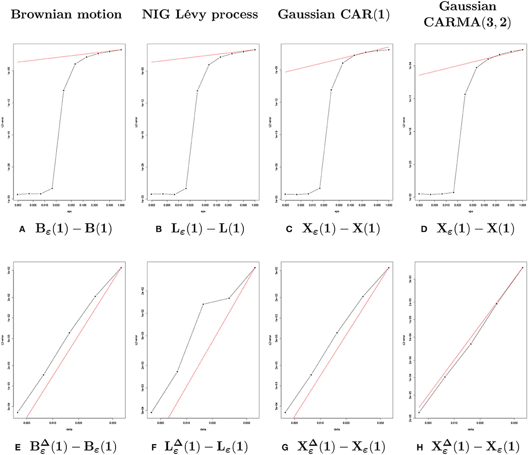
Figure 3. Log-log plots for the squared approximation error after 1, 000 simulations. Above, the error is a function of ε with fixed Δ = 2⁻³. Below, the error is a function of Δ with fixed ε = 0.01.

3. CARMA Representation and Convergence Results

For p > q and t ≥ 0, a second-order Lévy-driven continuous-time ARMA process of order (p, q) is formally defined by the stochastic differential equation

$\begin{array}{ll}P\left(\frac{d}{dt}\right)X(t)=Q\left(\frac{d}{dt}\right)\frac{d}{dt}L(t),& (3.1)\end{array}$

where P and Q are the characteristic polynomials of the CARMA process of the form

$\begin{array}{l}P(z)=z^p+a_1{z}^{p-1}+\dots +a_p\\ Q(z)=b_0+b_{1}z+\dots +b_{p-1}{z}^{p-1}& (3.2)\end{array}$

with a_j ≥ 0, j = 1, …, p, and a_p > 0, b_q = 1 and b_j = 0 for q < j < p. Equation (3.1) is, however, usually interpreted by means of its state-space representation

$\begin{array}{ll}\{\begin{array}{c}d\text{Y}(t)=A\text{Y}(t)dt+{\text{e}}_{p}dL(t)\hfill \\ X(t)={\text{b}}^{\top }\text{Y}(t)\hfill \end{array},\hfill & (3.3)\end{array}$

where ⊤ denotes the transpose operator, and

$\begin{array}{l}A=\left(\begin{array}{ccccc}0& 1& 0& \cdots & 0\\ 0& 0& 1& \cdots & 0\\ ⋮& ⋮& ⋮& \ddots & ⋮\\ 0& 0& 0& \cdots & 1\\ -a_p& -a_{p-1}& -a_{p-2}& \cdots & -a_1\end{array}\right),{\text{ e}}_p=\left(\begin{array}{c}0\\ 0\\ ⋮\\ 0\\ 1\end{array}\right),\text{ b}=\left(\begin{array}{c}{b}_0\\ b_1\\ ⋮\\ b_{p-2}\\ b_{p-1}\end{array}\right).\end{array}$

By Itô's rule, the solution of the first equation in (3.3) at time t ≥ s is given by

$\begin{array}{l}\text{Y}(t)=e^{A(t-s)}\text{Y}(s)+{\displaystyle {\int }_s^t}{e}^{A(t-u)}{\text{e}}_{p}dL(u).\end{array}$

Moreover, from Brockwell et al. [5, Proposition 1], if the eigenvalues λ₁, …, λ_p of A satisfy the condition

$\begin{array}{ll}Re({\lambda }_j)<0\text{ for }j=1,\dots ,p,& (3.4)\end{array}$

then the process {Y(t), t ≥ 0} is strictly stationary and the CARMA(p, q) process is given by

$\begin{array}{ll}X(t)={\displaystyle {\int }_0^t}g(t-s)dL(s),& (3.5)\end{array}$

$\begin{array}{ll}g(x):={\text{b}}^{\top }{e}^{Ax}{\text{e}}_p,x\ge 0.& (3.6)\end{array}$

The function g is referred to as the kernel function associated to the CARMA process. We also notice that the process X is a causal function of L, in the sense that X(t) is independent of {L(s) − L(t), s ≥ t} for all t ≥ 0. We shall assume that condition (3.4) is satisfied, referring to it as the causality condition or stationarity condition.

In a similar way, we introduce the state-space representation for X_ε. This is the process obtained by replacing the Lévy process L with the smoother L_ε, namely

$\begin{array}{ll}\{\begin{array}{c}d{\text{Y}}_{\epsilon }(t)=A{\text{Y}}_{\epsilon }(t)dt+{\text{e}}_{p}d{L}_{\epsilon }(t)\hfill \\ X_{\epsilon }(t)={\text{b}}^{\top }{\text{Y}}_{\epsilon }(t)\hfill \end{array}.\hfill & (3.7)\end{array}$

The solution to Equation (3.7) can be expressed in terms of the kernel function g by

$\begin{array}{ll}{X}_{\epsilon }(t)={\displaystyle {\int }_0^t}g(t-s)d{L}_{\epsilon }(s).& (3.8)\end{array}$

We point out that the kernel function g in Equation (3.6) is continuously differentiable. Its value at x = 0 is given in the following lemma, where δ denotes the Kronecker delta.

Lemma 3.1. For p > q, the value of the kernel function at x = 0 is equal to g(0) = δ_p,q+1.

Proof: The proof follows by direct verification.□

From the basic algebra analysis, if A has distinct eigenvalues, then the matrix exponential e^Ax can be decomposed into the matrix product

$\begin{array}{ll}{e}^{Ax}=V{e}^{\Lambda x}{V}^{-1},& (3.9)\end{array}$

Λ and V being the eigenvalues and eigenvectors matrices. From Brockwell et al. [5, Remark 2], the eigenvalues λ₁, …, λ_p of the matrix A coincide with the roots of the polynomial P in Equation (3.2), and the i-th eigenvector is of the form $v_i={\left[1,{\lambda }_i,{\lambda }_i^2,\dots ,{\lambda }_i^{p-1}\right]}^{\top }$. From Brockwell et al. [5, Proposition 2], we also get that $V^{-1}{\text{e}}_p={\left[{\gamma }_1,{\gamma }_2,\dots ,{\gamma }_p\right]}^{\top }$, where

$\begin{array}{ll}{\gamma }_i:=\frac{1}{P^{\prime }({\lambda }_i)}=\frac{1}{{\displaystyle {\prod }_{\begin{array}{c}1\le m\le p\\ m\ne i\end{array}}}({\lambda }_i-{\lambda }_m)}\text{ for }i=1,\dots ,p,& (3.10)\end{array}$

P′ being the derivative of the polynomial P. We then find the following spectral representations for the kernel function g and its first derivative h(x): = g′(x).

Lemma 3.2. The functions g and h can be expressed in terms of the spectral representations:

$\begin{array}{l}g(x)={\displaystyle \sum _{i,j=1}^p}{b}_j{\lambda }_i^j{\gamma }_i{e}^{{\lambda }_{i}x}andh(x)={\displaystyle \sum _{i,j=1}^p}{\tilde{b}}_j{\lambda }_i^j{\gamma }_i{e}^{{\lambda }_{i}x},\end{array}$

for γ_i in Equation (3.10), and ${\tilde{b}}_j={\left[{\text{b}}^{\top }A\right]}_j$, j = 1, …, p.

Proof: The proof comes from Equations (3.6) and (3.9) by writing explicitly the matrix product $g(x)={\text{b}}^{\top }V{e}^{\Lambda x}{V}^{-1}{\text{e}}_p$ and $h(x)=g^{\prime }(x)={\text{b}}^{\top }AV{e}^{\Lambda x}{V}^{-1}{\text{e}}_p$.□

These representations will be used for proving the convergence results in the next section.

3.1. Convergence of the CARMA Approximation

We prove the convergence of X_ε to X. We first start with the following preliminary result.

Lemma 3.3. The processes {X(t), t ≥ 0} and {X_ε(t), t ≥ 0} can be rewritten by

$\begin{array}{l}X(t)={\displaystyle {\int }_0^t}h(t-s)L(s)dsand{X}_{\epsilon }(t)={\displaystyle {\int }_0^t}{h}_{\epsilon }(t-s)L(s)ds.\end{array}$

Here h(x) = g′(x) and $h_{\epsilon }(x):=g(0){\psi }_{\epsilon }(x)+{\int }_0^{x}h(x-v){\psi }_{\epsilon }(v)dv$, for g(0) given in Lemma 3.1.

Proof: See Appendix A.5 in Supplementary Material.

From Lemma 3.2, we also derive the spectral representation

$\begin{array}{ll}{h}_{\epsilon }(x)=g(0){\psi }_{\epsilon }(x)+{\displaystyle \sum _{i,j=1}^p}{\tilde{b}}_j{\lambda }_i^j{\gamma }_i{\displaystyle {\int }_0^x}{e}^{{\lambda }_i(x-v)}{\psi }_{\epsilon }(v)dv,& (3.11)\end{array}$

and prove the first convergence result.

Proposition 3.4. For every x > 0, the function h_ε(x) converges pointwise to h(x).

Proof: See Appendix A.6 in Supplementary Material.

In Proposition 3.4, we do not require the limit to hold in x = 0. However, this does not affect the convergence in L² since X and X_ε are both integral functions, and {x = 0} is a set of measure 0. Indeed, we can prove the required convergence for X_ε.

Theorem 3.5. The process {X_ε(t), t ≥ 0} converges to {X(t), t ≥ 0} in L²([0, T] × Ω).

Proof: See Appendix A.7 in Supplementary Material.

Figure 4 shows the convergence proven in Theorem 3.5 for a Gaussian CAR(1) process with parameter a = 0.6. We notice that X_ε captures the shape of X even with ε large, and we observe a right-shifting of X_ε with respect to X, as noticed already for the Lévy process approximation.

FIGURE 4

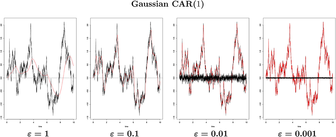
Figure 4. The Gaussian CAR(1) process {X(t), 0 ≤ t ≤ 10} (black line) with parameter a = 0.6 against {X_ε(t), 0 ≤ t ≤ 10} (red line) for different ε's generated from a single path with Δ^true = 2⁻¹⁰ (n = 10, 240 points). The black bar lines in the two rightmost images represent the difference between X and X_ε.

We now study explicitly the rate of convergence of X_ε to the CARMA process X.

Proposition 3.6. For every ε > 0 and T < +∞, there exists a constant K₂ > 0 such that

$\begin{array}{l}𝔼\left[{\left(X_{\epsilon }(T)-X(T)\right)}^2\right]\le K_2{\epsilon }^2+O({\epsilon }^3).\end{array}$

Proof: See Appendix A.8 in Supplementary Material.

The rate of convergence obtained in Proposition 3.6 is shown in Figure 3C for a CAR(1).

We point out that the results in this section have been stated and proved for a general CARMA(p, q) process. The convergence results are indeed valid for every q ≥ 0, even when L_ε is not smooth enough to make the SDE having mathematical sense. We then present them for the general case. Since the same ideas apply to other families of convolution functions, such as the Gamma densities previously mentioned, this is useful for possible further applications.

We end this section with a distribution property holding for X_ε when the original noise is driven by a Brownian motion. If the CARMA process X is driven by a Brownian motion B, then X has Gaussian distribution. We show that the same holds for X_ε. This is indeed not a straightforward result since the process B_ε is no longer a Brownian motion by means of Proposition 2.2. A rigorous proof is thus necessary.

Proposition 3.7. For every ε > 0, the process {X_ε(t), t ≥ 0} has Gaussian distribution.

Proof: See Appendix A.9 in Supplementary Material.

3.2. When q > 0

The process L_ε is continuously differentiable but is not twice continuously differentiable. However, at the right-hand side of the stochastic differential equation (3.1), we require q + 1 derivatives of the driving noise process. For the general case q > 0 we need the following result.

Proposition 3.8. Under the causality condition (3.4) and if the matrix A has distinct eigenvalues, the CARMA(p, q) process X can be expressed by the sum

$\begin{array}{l}X(t)={\displaystyle \sum _{r=1}^p}{X}^{(r)}(t)with\\ X^{(r)}(t):={\displaystyle {\int }_0^t}{\alpha }_r{e}^{{\lambda }_r(t-u)}dL(u),r=1,\dots ,p.\end{array}$

Here, the X^(r) are dependent and possibly complex-valued CAR(1) processes with ${\alpha }_r:=\frac{Q({\lambda }_r)}{P^{\prime }({\lambda }_r)}$.

Proof: See [5, Proposition 2].

By means of Proposition 3.8, starting from L_ε in Equation (2.3), the idea is to construct p-approximating processes and obtain X_ε as the sum of them, namely,

$\begin{array}{l}{X}_{\epsilon }(t)={\displaystyle \sum _{r=1}^p}{X}_{\epsilon }^{(r)}(t)\text{ with}\\ X_{\epsilon }^{(r)}(t)={\displaystyle {\int }_0^t}{\alpha }_r{e}^{{\lambda }_r(t-u)}d{L}_{\epsilon }(u),r=1,\dots ,p.\end{array}$

In particular, from Itô's calculus, we can prove that, for any r = 1, …, p and t ≥ 0, the process X^(r), respectively $X_{\epsilon }^{(r)}$, satisfies the stochastic differential equation

$\begin{array}{ll}d{X}_{(\epsilon )}^{(r)}(t)={\lambda }_r{X}_{(\epsilon )}^{(r)}(t)dt+{\alpha }_{r}d{L}_{(\epsilon )}(t),& (3.12)\end{array}$

that will be used for numerical purposes in section 4. In Equation (3.12), we write ε in parentheses since it applies to both X^(r) and $X_{\epsilon }^{(r)}$.

In Figure 5 we consider a Gaussian CARMA(3, 2) process with parameters (a₁, a₂, a₃) = (2.043, 1.339, 0.177) taken from [6] where a CAR(3) is used to model the daily average temperature dynamics in Stockholm (Sweden) and (b₀, b₁, b₂) = (2.0, 0.8, 1.0). In Figure 3D, we observe the rate of convergence as a function of ε.

FIGURE 5

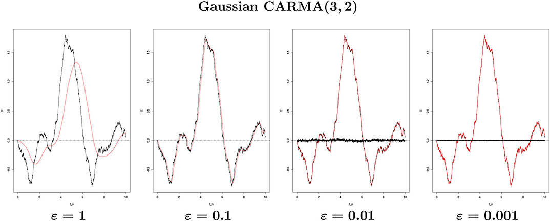
Figure 5. The Gaussian CARMA(3, 2) process {X(t), 0 ≤ t ≤ 10} (black line) with parameters (a₁, a₂, a₃, b₀, b₁, b₂) = (2.043, 1.339, 0.177, 2.0, 0.8, 1.0) against {X_ε(t), 0 ≤ t ≤ 10} (red line) for different ε's generated from a single path with Δ^true = 2⁻¹⁰ (n = 10, 240 points). The black bar lines in the two rightmost images represent the difference between X and X_ε.

4. Numerical Schemes and Results

We consider a possible approach to simulate X and X_ε for some CARMA parameters, and we then estimate these parameters starting from the simulated time series. In particular, we need first to simulate L, then L_ε, and only afterwards can we simulate X_ε. For n > 0, we shall consider the partition $\Pi (n):=\left\{0=s_0^{(n)}<s_1^{(n)}<\cdots <s_n^{(n)}=T\right\}$ such that $\Delta s_j^{(n)}:=s_j^{(n)}-s_{j-1}^{(n)}$ is constant, that is $\Delta s_j^{(n)}=T/n=\Delta (n)=:\Delta$, and $s_j^{(n)}=j\Delta$ for each j = 0, …, n.

4.1. The Lévy Simulations

By definition, for a fixed time interval Δ, the increments of the Lèvy process $\Delta L(s_j^{(n)}):=L(s_j^{(n)})-L(s_{j-1}^{(n)})$, j = 1, …, n, are independent and identically distributed random variables following a certain distribution, which depends only on the time increment Δ. For example, for L = B, the increments $\Delta B(s_j^{(n)})$ have all Gaussian distribution with zero mean and variance Δ. A possible approach to simulate L_ε in an exact way is to find the distribution of L_ε(t), starting from the distribution of L(t). For example, for L = B, by means of Lemma 2.3, we can simulate B_ε sampling directly from a Gaussian distribution with zero mean and variance in Lemma 2.3. However, with this approach, L and L_ε are from two different ω's in Ω, and comparing the two paths we would not get the error measure required. We then need an alternative approach that simulates L_ε and L from the same ω ∈ Ω.

From Equation (2.3), L_ε is the stochastic integral of ϕ_ε with respect to the Lévy process L. From the definition of the stochastic integral as a limit of approximating Riemann-Stieltjes sums [20], for t ∈ Π(n) such that $t=s_m^{(n)}=m\Delta$, for m = m(t) and 1 ≤ m ≤ n, we approximate L_ε(t) by approximating the integral with a sum, namely

$\begin{array}{l}{L}_{\epsilon }(t)={\displaystyle {\int }_0^t}{\varphi }_{\epsilon }(t-s)dL(s)\\ \begin{array}{l}\approx {\displaystyle \sum _{j=1}^m}{\varphi }_{\epsilon }(t-s_{j-1}^{(n)})\Delta L(s_j^{(n)})=:L_{\epsilon }^{\Delta }(t),\end{array}& (4.1)\end{array}$

where $t-s_{j-1}^{(n)}=(m+1-j)\Delta =s_{m+1-j}^{(n)}$. The approximation scheme (4.1) adds an error to the simulation. It, however, constructs L_ε starting from the simulations of L, allowing to compare the two paths for different Δ's. In the next proposition, we study the approximation error.

Proposition 4.1. For every Δ > 0, ε > 0 and T < +∞, there exists a constant K₃ > 0 such that the simulation error is bounded by

$\begin{array}{l}𝔼\left[{\left(L_{\epsilon }^{\Delta }(T)-L_{\epsilon }(T)\right)}^2\right]\le K_3\frac{{\Delta }^2}{\epsilon }.\end{array}$

Proof: See Appendix A.10 in Supplementary Material.

With Proposition 4.1, we estimated an upper bound for the error added by the Euler scheme for simulating the process L_ε by means of the process $L_{\epsilon }^{\Delta }$. In particular, it shows that, for a fixed ε > 0, the simulation error decreases at the decreasing of the time step Δ, as we would expect. In Kloeden et al. [21, section 9.3], the authors study the rate of convergence for the Euler scheme when applied to an Itô process, with respect to the absolute error criterion, finding a strong rate of convergence equal to 1/2. Here, in line with the rest of the paper, we consider the squared error in Proposition 4.1 instead. This gives a rate of convergence equal to 2, corresponding to a strong order 1. From Proposition 4.1, we also notice that the bound depends on the inverse of ε, meaning that, for ε going to zero, the simulation error might explode.

Figure 5 shows the convergence of the Euler scheme (4.1) for a Brownian motion and for the normal inverse Gaussian process introduced in section 2.1. Since an exact simulation is not possible, to generate B_ε, we consider the scheme (4.1) with a small time step Δ^true = 2⁻¹⁰. Moreover, since we want to compare B_ε and $B_{\epsilon }^{\Delta }$ path-wise for different values of Δ, B_ε and $B_{\epsilon }^{\Delta }$ must be related to the same ω ∈ Ω, that is, to the same realization of the Brownian motion B. To get this, we exploit the following well-known property: given $X_i~{N}(0,{\sigma }_i^2)$, for i = 1, …, k, independent Gaussian random variables, their sum follows the distribution $\sum _{i=1}^k{X}_i~{N}(0,\sum _{i=1}^k{\sigma }_i^2)$. Thus, we start by simulating the true process B_ε for a certain time step Δ^true << 1. For this, we sample the increments $\Delta B(s_j^{(n)})$ from a Gaussian distribution with zero mean and variance Δ^true and obtain B_ε as in Equation (4.1). Then, we choose a time step Δ multiple of Δ^true, namely, Δ = kΔ^true for a certain k ∈ ℕ. The Brownian motion path to be used in Equation (4.1) for simulating $B_{\epsilon }^{\Delta }$ is then obtained by summing up the increments of B (above simulated) at groups of k elements. These increments have indeed Gaussian distribution with zero mean and variance $\sum _{i=1}^k{\Delta }^{true}=k{\Delta }^{true}=\Delta$, as required. In Figure 6, we considered Δ^true = 2⁻¹⁰ and Δ ∈ {2⁻⁷, 2⁻⁵, 2⁻³, 2⁻¹}. We see that, for a fixed ε, as Δ decreases, the error between $B_{\epsilon }^{\Delta }$ and B_ε decreases. Even with a large Δ (Δ = 2⁻¹), the process $B_{\epsilon }^{\Delta }$ captures the shape of B_ε. In Figure 3E we show the rate of convergence of the Euler scheme proven in Proposition 4.1 as function of time step Δ and for a fixed ε (ε = 0.01).

FIGURE 6

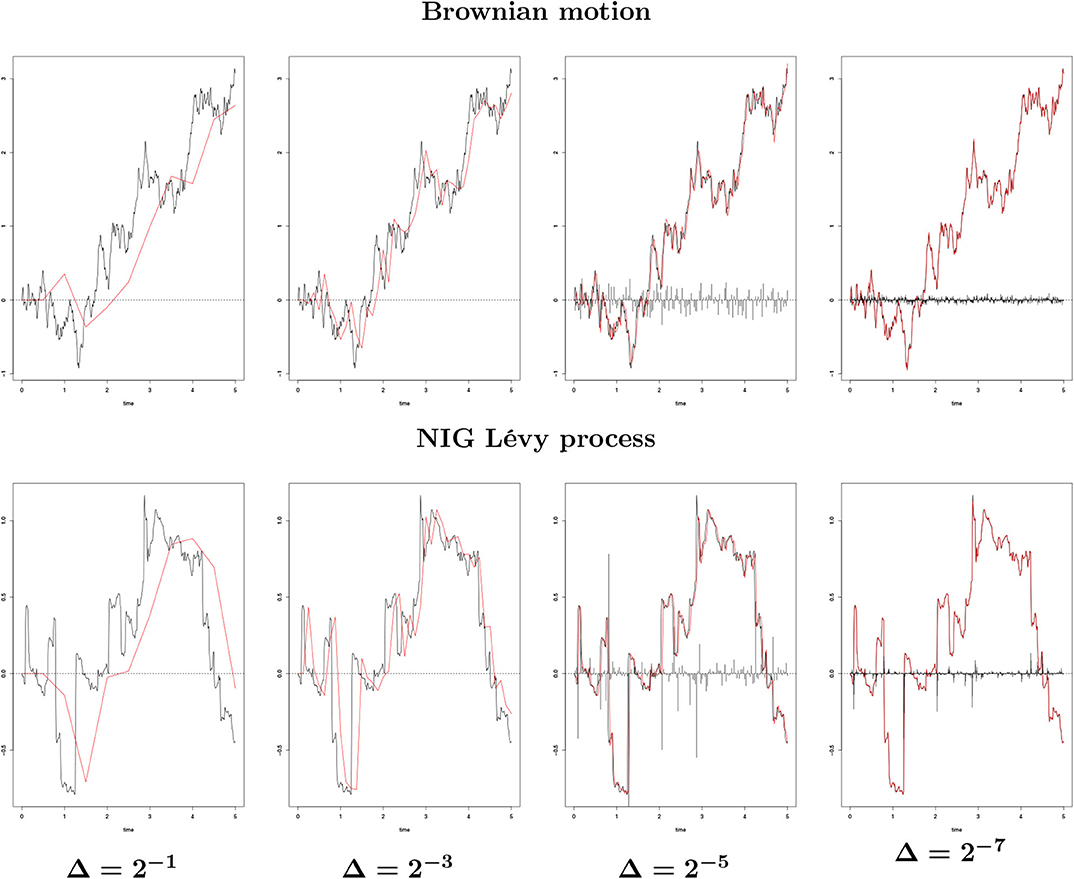
Figure 6. {L_ε(t), 0 ≤ t ≤ 5} (black line) against $\left\{L_{\epsilon }^{\Delta }(t),0\le t\le 5\right\}$ (red line) for different Δ's generated from a single path with ε = 0.01, for a Brownian motion and an NIG process with parameters (α, β, δ, μ) = (1, 0, Δ^true, 0). The black bar lines in the four rightmost images represent the difference between L_ε and $L_{\epsilon }^{\Delta }$.

Similarly, for the NIG Lévy process, to simulate and compare L_ε with $L_{\epsilon }^{\Delta }$ path-wise, we use the same idea as in the Brownian motion case. We can indeed exploit the convolution property of the NIG distribution (see [22]): given X_i ~ NIG(α, β, δ_i, μ_i), for i = 1, …, k, independent normal inverse Gaussian random variables with common parameters α and β, but individual scale-location parameters δ_i and μ_i, their sum follows $\sum _{i=1}^k{X}_i~\text{NIG}(\alpha ,\beta ,\sum _{i=1}^k{\delta }_i,\sum _{i=1}^k{\mu }_i)$. In section 2.1, we introduced NIG distribution with parameters (1, 0, Δ^true, 0), for Δ^true being the time step used in the Euler discretization. As above, we thus simulate the true process L_ε from Equation (4.1) by sampling the increments of L from a NIG distribution with parameters (1, 0, Δ^true, 0) for a certain Δ^true << 1. Then, we obtain $L_{\epsilon }^{\Delta }$ by choosing Δ so that Δ = kΔ^true for a certain k ∈ ℕ, and summing up the increments of L (simulated above) at groups of k elements. These increments have indeed NIG distribution with parameters $(1,0,\sum _{i=1}^k{\Delta }^{true},\sum _{i=1}^{k}0)=(1,0,\Delta ,0)$ as required. We consider the same Δ's as for the Brownian motion. We notice that, for a fixed ε, $L_{\epsilon }^{\Delta }$ captures the shape of L_ε even with a large Δ. In Figure 3F we show the rate of convergence for the Euler scheme proved in Proposition 4.1 as function of the time step Δ and for a fixed ε (ε = 0.01).

From Proposition 2.7 and 4.1, we calculate the squared error for $L_{\epsilon }^{\Delta }$ with respect to L.

Proposition 4.2. For every Δ > 0 and ε > 0 small enough, we get the following bound

$\begin{array}{l}𝔼\left[{\left(L_{\epsilon }^{\Delta }(T)-L(T)\right)}^2\right]\le 2K_1\epsilon +2K_3\frac{{\Delta }^2}{\epsilon }.\end{array}$

Proof: This is a direct consequence of Proposition 2.7 and 4.1 by the inequality (a + b)² ≤ 2(a² + b²) for $a=L_{\epsilon }^{\Delta }(T)-L_{\epsilon }(T)$ and b = L_ε(T) − L(T).□

Proposition 4.2 shows that the squared error between $L_{\epsilon }^{\Delta }$ and L decreases when Δ decreases. However, because of the term proportional to the inverse of ε, it might also explode for small values of ε. We then need to tune the parameters Δ and ε to find a combination that minimizes the error preventing it from taking large values.

4.2. The CARMA Simulations

It is possible to construct X and X_ε starting from Equations (3.5) and (3.8) and considering the same kind of numerical approximation as done for L_ε, that is, by replacing the integral with a suitable sum. However, to not add a second simulation error to the one already due to L_ε, which is approximated by $L_{\epsilon }^{\Delta }$, we start from the state-space representations instead, Equations (3.3) and (3.7), respectively. By using the Euler scheme, according to [21, Chapter 9], we get (here we write ε in parenthesis since the equation holds both for X and X_ε):

$\begin{array}{l}{\text{Y}}_{(\epsilon )}^{\Delta }(s_j^{(n)})={\text{Y}}_{(\epsilon )}^{\Delta }(s_{j-1}^{(n)})+A{\text{Y}}_{(\epsilon )}^{\Delta }(s_{j-1}^{(n)})\Delta +{\text{e}}_p\Delta L_{(\epsilon )}(s_j^{(n)}),\\ X_{(\epsilon )}^{\Delta }(s_j^{(n)})={\text{b}}^{\top }{\text{Y}}_{(\epsilon )}^{\Delta }(s_j^{(n)}),& (4.2)\end{array}$

where $\Delta L_{(\epsilon )}(s_j^{(n)})=L_{(\epsilon )}(s_j^{(n)})-L_{(\epsilon )}(s_{j-1}^{(n)})$, for j = 1, …, n. For the reasons already discussed, we apply the scheme (4.2) only for q = 0, that is, when b = e₁. For q > 0, by means of Proposition 3.8, we instead apply the Euler scheme to the stochastic differential equation (3.12) for each of the p components $X_{(\epsilon )}^{(r)}$ of X_(ε), and we get X_(ε) as the sum of them, namely,

$\begin{array}{l}{X}_{(\epsilon )}^{\Delta (r)}(s_j^{(n)})=X_{(\epsilon )}^{\Delta (r)}(s_{j-1}^{(n)})+{\lambda }_r{X}_{(\epsilon )}^{\Delta (r)}(s_{j-1}^{(n)})\Delta +{\alpha }_r\Delta L_{(\epsilon )}(s_j^{(n)}),\\ X_{(\epsilon )}^{\Delta }(s_j^{(n)})={\displaystyle \sum _{r=1}^p}{X}_{(\epsilon )}^{\Delta (r)}(s_j^{(n)}).\end{array}$

When simulating $X_{\epsilon }^{\Delta }$, we use the approximation $L_{\epsilon }^{\Delta }$ in Equation (4.1), and this adds an error. We study the rate of convergence for $X_{\epsilon }^{\Delta }$ to the true process X_ε in the following proposition.

Proposition 4.3. For every ε > 0 and $\Delta <{\text{max}}_{j=1,\dots ,p}\frac{-2Re({\lambda }_j)}{|{\lambda }_j{|}^2}$, there exist two constants K₄, K₅ > 0 such that the simulation error for the Euler scheme (4.2) is bounded by

$\begin{array}{l}𝔼\left[{\left(X_{\epsilon }^{\Delta }(T)-X_{\epsilon }(T)\right)}^2\right]\le K_4\frac{{\Delta }^2}{\epsilon }+K_5\frac{{\Delta }^4}{{\epsilon }^4}.\end{array}$

Proof: See Appendix A.11 in Supplementary Material.

Let us notice that the bound on Δ in Proposition 4.3 has been introduced to obtain the estimate for the squared error. The scheme (4.2) works however for every Δ > 0.

In Figure 7 we show the convergence for the simulations of a Gaussian CAR(1) and a Gaussian CARMA(3, 2). In both cases we notice that for Δ decreasing, the Euler approximation $X_{\epsilon }^{\Delta }$ converges to X_ε, and, even with a large value of Δ (Δ = 2⁻¹), $X_{\epsilon }^{\Delta }$ captures the shape of X_ε. In Figures 3G,H, we show the rate of convergence for the two processes as function of Δ² and for a fixed value of ε (ε = 0.01).

FIGURE 7

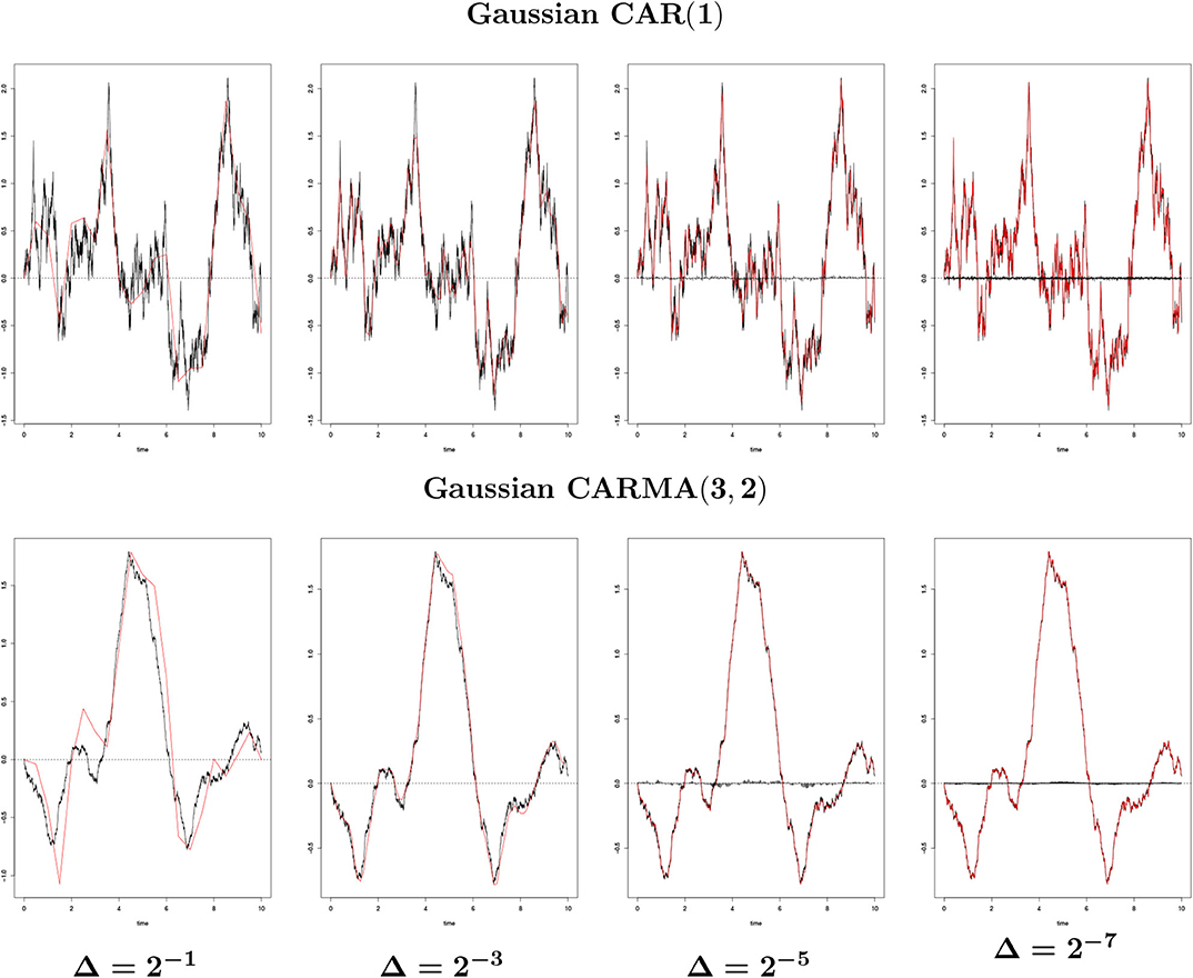
Figure 7. {X_ε(t), 0 ≤ t ≤ 10} (black line) against $\left\{X_{\epsilon }^{\Delta }(t),0\le t\le 10\right\}$ (red line) for different Δ's generated from a single path and ε = 0.01, for X a Gaussian CAR(1) with parameter a = 0.6 and a Gaussian CARMA(3, 2) with parameters (a₁, a₂, a₃, b₀, b₁, b₂) = (2.043, 1.339, 0.177, 2, 0.8, 1). The black bar lines in the four rightmost images represent the difference between X_ε and $X_{\epsilon }^{\Delta }$.

From Proposition 3.6 and 4.3, we estimate the squared error for $X_{\epsilon }^{\Delta }$ with respect to X.

Proposition 4.4. For every Δ > 0 and ε > 0 small enough, the following bound applies:

$\begin{array}{l}𝔼\left[{\left(X_{\epsilon }^{\Delta }(T)-X(T)\right)}^2\right]\le 2K_2{\epsilon }^2+2K_4\frac{{\Delta }^2}{\epsilon }+2K_5\frac{{\Delta }^4}{{\epsilon }^4}.\end{array}$

Proof: This is a direct consequence of Proposition 3.6 and 4.3 by the inequality (a + b)² ≤ 2(a² + b²) for $a=X_{\epsilon }^{\Delta }(T)-X_{\epsilon }(T)$ and b = X_ε(T) − X(T).□

4.3. CARMA Estimation

We introduce an approach to estimate the parameters (a₁, …, a_p, b₀, …, b_q) starting from the time series for {X(t), 0 ≤ t ≤ T} and {X_ε(t), 0 ≤ t ≤ T} by applying the Euler scheme. Following Benth et al. [7, section 4.3], we focus on CAR models only, that is, on the process X(t) = Y₁(t), for Y₁(t) being the first coordinate of the vector Y(t) in Equation (3.3). Then, for a uniform time step Δ, we get the relation

$\begin{array}{l}\frac{1}{{\Delta }^{p-1}}{\displaystyle \sum _{j=0}^p}{(-1)}^j{z}_j^p{Y}_1(t+(p-j)\Delta )=\\ \begin{array}{c}=-{\displaystyle \sum _{i=1}^p}{a}_{p-i+1}\frac{1}{{\Delta }^{i-2}}{\displaystyle \sum _{j=0}^{i-1}}{(-1)}^j{z}_j^{i-1}{Y}_1(t+(i-1-j)\Delta )+ϵ(t),\end{array}& (4.3)\end{array}$

ϵ(t) being the Lévy noise. The coefficients $z_j^i$ are defined as $z_0^i=z_i^i=1$ for i = 1, …, p, and, through the recursion $z_j^i=z_{j-1}^{i-1}+z_j^{i-1}$, for j = 1, …, p−1 and i ≥ 2. We refer to Benth et al. [7, section 4.3] for more details. In particular, Equation (4.3) is a linear combination of Y₁(t + pΔ), …, Y₁(t) and the error term ϵ(t). Thus, we have an AR(p) representation model for Y₁(t), and the parameters a₁, …, a_p can be estimated by means of relation (4.3) starting from the AR estimated parameters. We consider as examples p = 1 and p = 3. For p = 1, X(t) = Y₁(t) is an Ornstein-Uhlenbeck process and Equation (4.3) becomes

$\begin{array}{l}{Y}_1(t+\Delta )=\left\{1-a_1\Delta \right\}{Y}_1(t)+ϵ(t),\end{array}$

which coincides with the Euler scheme (4.2) when p = 1. For p = 3, from Equation (4.3) we get

$\begin{array}{l}\frac{1}{{\Delta }^2}\{z_0^3{Y}_1(t+3\Delta )-z_1^3{Y}_1(t+2\Delta )+\\ +z_2^3{Y}_1(t+\Delta )-z_3^3{Y}_1(t)\}\\ =-a_3\Delta z_0^0{Y}_1(t)-a_2\left\{z_0^1{Y}_1(t+\Delta )-z_1^1{Y}_1(t)\right\}+\\ -\frac{a_1}{\Delta }\left\{z_0^2{Y}_1(t+2\Delta )-z_1^2{Y}_1(t+\Delta )+z_2^2{Y}_1(t)\right\}+ϵ(t).\end{array}$

From the definition for $z_j^i$, rearranging the terms, the last equation can be rewritten as

$\begin{array}{l}{Y}_1(t+3\Delta )={\theta }_1{Y}_1(t+2\Delta )+{\theta }_2{Y}_1(t+\Delta )+{\theta }_3{Y}_1(t)+{\Delta }^2ϵ(t),\\ \text{ with }{\theta }_1:=3-a_1\Delta ,{\theta }_2:=2a_1\Delta -a_2{\Delta }^2-3,\\ {\theta }_3:=1-a_1\Delta +a_2{\Delta }^2-a_3{\Delta }^3.\end{array}$

Then, one first estimates the AR coefficients θ₁, θ₂, θ₃ and afterwards recover the CAR coefficients a₁, a₂, a₃ by

$\begin{array}{l}{a}_1=\frac{3-{\theta }_1}{\Delta },a_2=\frac{3-2{\theta }_1-{\theta }_2}{{\Delta }^2},a_3=\frac{1-{\theta }_1-{\theta }_2-{\theta }_3}{{\Delta }^3}.\end{array}$

This scheme holds for every Lévy process. To recover the case q > 0 different approaches have to be considered, see, e.g., [23] and [24].

In Tables 1, 2 we report the parameters estimated for a Gaussian CAR(1) and a Gaussian CAR(3) for different ε's and different Δ's. In particular, â is the vector of parameters estimated starting from the time series for X, and â_ε is the vector of parameters estimated starting from the time series for X_ε. The underlined digits are the common digits between â and â_ε, with respect to the same ε and the same Δ. The estimates get more accurate for a small ε, but they are not accurate if ε is bigger than Δ. We marked the cases corresponding to ε < Δ with the symbol *, and we notice that as soon as ε gets smaller than Δ, the accuracy improves and gets better for smaller values of ε. We summarize this empirical result with a proposition.

TABLE 1

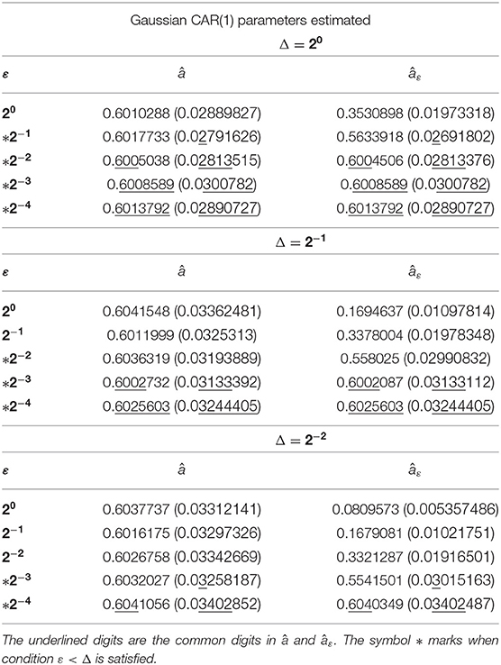
Table 1. Parameters estimated and standard deviation (in parenthesis) for different ε's and Δ's after 1, 000 simulations for a Gaussian CAR(1) with a = 0.6.

TABLE 2

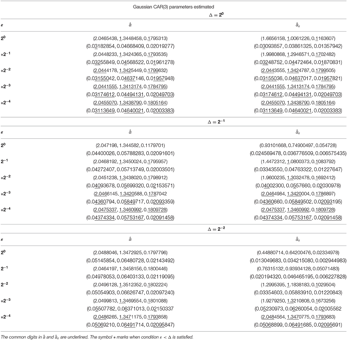
Table 2. Parameters estimated and standard deviation (every second row) for different ε's and Δ's after 1, 000 simulations for a Gaussian CAR(3) with a = (2.043, 1.339, 0.177).

Proposition 4.5. The Euler scheme (4.3) converges to the true CARMA parameters if ε < Δ.

Proof: See Appendix A.12 in Supplementary Material.

A more rigorous study should be performed regarding the condition in Proposition 4.5, analysing in details the estimation technique for ARMA processes, which is the starting point to estimate the CARMA parameters. This is, however, beyond the purposes of the current article.

Data Availability Statement

The original contributions presented in the study are included in the article/Supplementary Material, further inquiries can be directed to the corresponding author.

Author Contributions

The author confirms being the sole contributor of this work and has approved it for publication.

Conflict of Interest

The author declares that the research was conducted in the absence of any commercial or financial relationships that could be construed as a potential conflict of interest.

Acknowledgments

The author acknowledges Fred Espen Benth for the several fruitful discussions that let to this paper and two referees for additional interesting comments.

Supplementary Material

The Supplementary Material for this article can be found online at: https://www.frontiersin.org/articles/10.3389/fams.2020.00037/full#supplementary-material

References

1. Brockwell PJ. Lévy-driven CARMA processes. Ann Inst Stat Math. (2001) 53:113–24. doi: 10.1023/A:1017972605872

CrossRef Full Text | Google Scholar

2. Barndorff-Nielsen OE, Shepard N. Non-Gaussian OU based models and some of their uses in financial economics. J R Stat Soc B Stat Methodol. (2001) 63:167–241. doi: 10.1111/1467-9868.00282

CrossRef Full Text | Google Scholar

3. Brockwell PJ, Marquardt T. Lévy-driven and fractionally integrated ARMA processes with continuous time parameter. Stat Sin. (2005) 15:477–94. Available online at: https://www.jstor.org/stable/24307365

Google Scholar

4. Brockwell PJ, Davis RA, Yang Y. Estimation for nonnegative Lévy-driven Ornstein-Uhlenbeck processes. J Appl Probab. (2007) 44:977–89. doi: 10.1239/jap/1197908818

CrossRef Full Text | Google Scholar

5. Brockwell PJ, Davis RA, Yang Y. Estimation for non-negative Lévy-driven CARMA processes. J Bus Econ Stat. (2011) 29:250–9. doi: 10.1198/jbes.2010.08165

CrossRef Full Text | Google Scholar

6. Benth FE, Benth JS, Koekebakker S. Stochastic Modelling of Electricity and Related Markets. Vol. 11. Singapore: World Scientific (2008).

Google Scholar

7. Benth FE, Benth JS. Modelling and Pricing in Financial Markets for Weather Derivatives. Vol. 17. Singapore: World Scientific (2012).

Google Scholar

8. Marquardt T. Fractional Lévy processes with an application to long memory moving average processes. Bernoulli. (2006) 12:1099–126. doi: 10.3150/bj/1165269152

CrossRef Full Text | Google Scholar

9. Marquardt T, James LF. Generating Long Memory Models Based on CARMA Processes. Technical report (2007).

Google Scholar

10. Paschke R, Prokopczuk M. Integrating multiple commodities in a model of stochastic price dynamics. J Energy Markets. (2009) 2:47–82. doi: 10.21314/JEM.2009.025

CrossRef Full Text | Google Scholar

11. Paschke R, Prokopczuk M. Commodity derivatives valuation with autoregressive and moving average components in the price dynamics. J Bank Finance. (2010) 34:2742–52. doi: 10.1016/j.jbankfin.2010.05.010

CrossRef Full Text | Google Scholar

12. Schwartz E, Smith JE. Short-term variations and long-term dynamics in commodity prices. Manage Sci. (2000) 46:893–911. doi: 10.1287/mnsc.46.7.893.12034

CrossRef Full Text | Google Scholar

13. Benth FE, Koekebakker S. Pricing of forwards and other derivatives in cointegrated commodity markets. Energy Econ. (2015) 52:104–17. doi: 10.1016/j.eneco.2015.09.009

CrossRef Full Text | Google Scholar

14. Benth FE, Klüppelberg C, Müller G, Vos L. Futures pricing in electricity markets based on stable CARMA spot models. Energy Econ. (2014) 44:392–406. doi: 10.1016/j.eneco.2014.03.020

CrossRef Full Text | Google Scholar

15. García I, Klüppelberg C, Müller G. Estimation of stable CARMA models with an application to electricity spot prices. Stat Model. (2011) 11:447–70. doi: 10.1177/1471082X1001100504

CrossRef Full Text | Google Scholar

16. Andresen A, Benth FE, Koekebakker S, Zakamulin V. The CARMA interest rate model. Int J Theor Appl Finance. (2014) 17:1450008. doi: 10.1142/S0219024914500083

CrossRef Full Text | Google Scholar

17. Adland R, Benth FE, Koekebakker S. Multivariate modeling and analysis of regional ocean freight rates. Transport Res E. (2018) 113:194–221. doi: 10.1016/j.tre.2017.10.014

CrossRef Full Text | Google Scholar

18. Cont R, Tankov P. Financial Modelling With Jump Processes. Chapman and Hall/CRC (2004).

Google Scholar

19. Benth FE, Di Persio L, Lavagnini S. Stochastic modelling of wind derivatives in energy markets. Risks. (2018) 6:56. doi: 10.3390/risks6020056

CrossRef Full Text | Google Scholar

20. Øksendal BK. Stochastic Differential Equations: An Introduction With Applications. 5th ed. Heidelberg; New York, NY: Springer-Verlag (2003).

Google Scholar

21. Kloeden PE, Platen E. Numerical Solution of Stochastic Differential Equation. Berlin; Heidelberg: Springer-Verlag (1992).

PubMed Abstract | Google Scholar

22. Hanssen A, Øigård TA. The normal inverse Gaussian distribution: a versatile model for heavy-tailed stochastic processes. In: 2001 IEEE International Conference on Acoustics, Speech, and Signal Processing. Proceedings. Vol. 6. Salt Lake City, UT (2001). doi: 10.1109/ICASSP.2001.940717

CrossRef Full Text | Google Scholar

23. Brockwell PJ, Davis RA. Introduction to Time Series and Forecasting. 2nd ed. New York, NY: Springer (2002). doi: 10.1007/b97391

CrossRef Full Text | Google Scholar

24. Stelzer R. CARMA processes driven by non-Gaussian noise. arXiv preprint arXiv:1201.0155 (2011).

Google Scholar