Estimating Dependence Among Lumber Strength Properties With Copula Models

1 Introduction

Lumber structural reliability is contingent upon setting and monitoring strict structural engineering design values for mechanical strength properties [1, 2]. Two crucial physical and mechanical structural properties are ultimate tensile strength (UTS) and modulus of rupture (MOR). UTS is defined as the maximum tensile stress that a lumber specimen can sustain in a direction parallel to the grain before failure. MOR is defined as the maximum bending stress that a lumber specimen can sustain before failure. A strong dependence between these two properties has important implications for monitoring and verification of strength properties. With strong dependence, not all the strength properties need to be tested. The cost of monitoring lumber reliability can be drastically reduced by leveraging dependence: measuring only one of the strength properties and predicting the other via their strong dependence.

The main contributions in this paper are a) description of an experimental design for measuring lumber strength properties with proof loading that allowed for estimation of dependence of destructively measured properties and graphical assessment of possible weakening due to proof loading and b) use of dependence models with flexible univariate margins and flexible bivariate copulas to summarize joint and conditional dependence. The structure of the experimental data led to part of the data being used for fitting the dependence models and other parts being used for sensitivity analysis and assessment of damage due to proof loading stress.

Both MOR and UTS are measured by destructive testing, which loads a lumber specimen on a specific strength testing machine until failure. Since a single lumber specimen cannot break twice, estimating the dependence of MOR and UTS is challenging as the two properties cannot be observed simultaneously. To address this issue, Refs. [3–5] introduce the first ever proof loading experiments designed to estimate dependence between the destructive lumber strength properties MOR and UTS. Proof loading is a technique used in the lumber industry to eliminate the weakest specimens in a population. It tests a specimen up to a predetermined load level and passes specimens through which do not fail at this level. The proposed experiment stresses each lumber specimen in either MOR or UTS mode up to a certain load level. The survivors are then tested to failure in whichever mode that has not been tested.

Unlike destructive strength properties such as MOR and UTS, elastic properties of lumber measure the bending deflection of a specimen caused by a low-level load, with the specimen completely recovering after measurement. One of the most common elastic properties of lumber is the vibration modulus of elasticity (MOE). A strong dependence between the elastic and strength properties has been demonstrated by various authors. Reference [6] considers different bivariate models such as bivariate Weibull and bivariate inverse Gaussian for MOR and MOE. Reference [7] fits a two-parameter Weibull distribution for MOR and a normal distribution for MOE and uses the bivariate Gaussian copula to model the dependence between MOR and MOE. The strong dependence between the elastic and strength properties can be used to infer the conditional dependence of MOR and UTS given MOE. Thus, Ref. [8] considers a trivariate normal distribution after log-transforming MOR, UTS, and MOE, instead of directly estimating the dependence between MOR and UTS with bivariate models. However, the normality assumption is very restrictive. A more flexible approach of constructing a trivariate distribution for the elastic and strength properties is preferred.

To leverage the proof loading technique and take the well-known fact that lumber specimens have elastic properties that are highly correlated with the strength properties into consideration, an experiment was designed and a copula-based method was implemented to estimate the joint dependence of MOR, UTS, and MOE. The designed experiment was conducted in the summer of 2011 at a wood processing lab located in FPInnovations. Lumber specimens were randomly divided into six proof loaded groups and two shoulder groups. The specimens of the shoulder groups were tested to failure in a tension or a bending machine. There are two kinds of proof loaded groups: specimens stressed with a bending machine in rupture mode to a certain bending load level, or specimens stressed with a tension machine in tension mode to a certain tension load level.

Using the resulting data of the summer-of-2011 experiment, the dependence of MOR, UTS, and MOE is modeled via a trivariate distribution constructed by a copula-based method. Estimation is done sequentially. After fitting appropriate univariate marginal distributions, the second step of the estimation finds appropriate copula families for i) the joint distributions of (MOR, MOE) and (UTS, MOE) and ii) the conditional distribution of (MOR, UTS) given MOE. This second step of the estimation is flexible and allows different dependence structures to be considered. We found strong conditional dependence between MOR and UTS given MOE.

In addition to estimating the joint dependence of MOR, UTS, and MOE, the summer-of-2011 experiment also allows us to assess whether proof loading led to weakening of the lumber specimens. References [8–10] assume that proof loading does not damage the lumber specimens. The no-damage assumption may well be unrealistic in certain situations, especially for the weaker specimens or when the proof loading level is high. The design of the summer-of-2011 experiment allows us to assess damage accumulated in one strength mode caused by proof loading in a second strength mode with predetermined load levels. The predetermined load levels are designed to fail 60, 40, and 20% of the specimens during the proof loading procedure. Our damage assessment indicates that there is damage to specimens due to proof loading, especially those specimens that are weaker. Surprisingly, a high proof load level does not necessarily imply damage. When specimens are proof loaded in the MOR mode with a high proof load that fails 60% of the specimens during the proof load procedure, our analysis suggests that the survivors’ UTS strengths are weakened. However, the same phenomenon is not observed on the survivors’ MOR strength when specimens are proof loaded in the UTS mode with a similar high load level setting; those survivors’ MOR strengths seem not to be weakened. Analyses in previous papers on the topic of lumber strength properties did not discuss potential weakening from proof loading.

The remainder of the article is organized as follows. In Section 2, we introduce the experiment and resulting lumber data set, together with an outline of the univariate analysis. In Section 3, a copula-based method is used to estimate the dependence among lumber properties under the experimental proof loading design. In Section 4, we present a graphical method for the copula models which takes into account possible weakening of lumber from the proof loading stage. This method suggests that there was some weakening. Section 5 has some concluding remarks, including how future experiments can better assess the weakening of lumber from proof loading.

2 Lumber Experiment for Measuring Strength Properties and Their Dependence

In this section, we introduce the summer-of-2011 experiment. The experiment and resulting data set are summarized from Refs. 11 and 12. This section also provides a summary of the univariate analysis for the three strength variables: MOR, UTS, and MOE.

2.1 The Summer-of-2011 Experiment

The lumber data set was experimentally collected in the summer of 2011. The experimental materials came in three bundles of lumber: two bundles labeled No. 1 and No. 2 were of grade-type SPF 1650f-1.5E, while one bundle labeled No. 3 was of type SPF No. 2. All the three bundles are mixtures from the Spruce, Pine, and Fir species. Eight hundred-seventy specimens from these three bundles were divided into eight experimental groups: R20/40/60/100 and T20/40/60/100. For all the experimental groups, the elastic property MOE was always measured and then adjusted for its moisture content following a standard procedure of American Standard Test Method D1990. Note that, for simplicity, MOE refers to adjusted MOE in the remainder of this article.

Groups R60/40/20 and T60/40/20 are called the proof loaded groups, where specimens were tested under different levels in the rupture mode and in the tension mode, respectively. Each group had 87 specimens. The MOE was always measured before proof loading.

For groups R60/40/20, specimens were first proof loaded in the rupture mode. If a specimen survived the rupture mode, it was then loaded to failure on the tension machine to measure its UTS. The experiment had been designed to fail 60, 40, and 20% of the specimens in the rupture mode for the R60, R40, and R20 groups, respectively. For a specimen in these three rupture mode proof loading groups, MOR was observed if the specimen failed due to proof loading in the rupture mode and UTS was observed otherwise.

Similarly, for groups T60/T40/T20, specimens were proof loaded in the tension mode. If a specimen survived the tension mode, it was then loaded to failure on the bending machine to measure its MOR. Again, 60/40/20 stands for the percentage of the lumber broken in the proof load procedure. For a specimen in these three tension mode proof loading groups, UTS was observed if the specimen failed due to proof loading in the tension mode and MOR was observed otherwise.

On the other hand, groups R100 and T100 are called the “shoulder groups,” and each had 174 specimens; the specimens in R100/T100 were loaded in a bending/tension machine, respectively, and tested to failure. Therefore, for group R100, MOE and MOR were measured. Similarly, for group T100, MOE and UTS were measured.

Related experiments were considered in earlier research. Reference [8] had data from two shoulder groups and one experimental group where specimens were proof loaded in the rupture mode to approximately the 40^th percentile with survivors tested to failure in the tension mode. Reference [5] had an experiment with specimens proof loading in the tension or the compression mode, and the survivors were tested to failure in the rupture mode. Our experiment is a symmetric design with the R and the T groups introduced above. The symmetric design strengthens the dependence signal between MOR and UTS provided by the proof loading techniques as suggested by [9] and demonstrated by [11]. In addition, our experiment does not only consider low load levels. The load levels range from failing 20–60% of the specimens during the proof loading procedures. The specification of the load levels enables us to quantify how the damage accumulated in the survivors as the proof load level increases.

2.2 Fitting Univariate Models for Strength Variables

Analysis with copula models usually involves two steps: the first step identifies and fits the univariate marginal distributions, and the second step fits appropriate copula families to represent the multivariate dependence structure. In this section, we summarize the univariate analyses for MOE, MOR, and UTS. The analysis is based on shoulder groups T100 and R100.

The summary statistics for MOR, UTS, and MOE based on groups R100 and T100 are given in Table 1. From both the histograms (not included here) of these variables and the summary statistics, it can be seen that the distributions of MOR and MOE are roughly symmetric, and the distribution of UTS is right-skewed.

TABLE 1

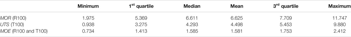
TABLE 1. Summary statistics for MOR, UTS, and MOE based on the R100 and T100 groups.

In previous papers discussing distributions for these three variables, Weibull, log-normal, and normal distributions have been used. The normal distribution is symmetric while the Weibull and log-normal distributions are right-skewed. To measure how well each of these three candidate distributions fits the collected data, we calculate the Akaike information criterion (AIC) values for the fitted Weibull, log-normal, and normal distributions for MOR, UTS, and MOE. The AIC measures a model’s suitability based on the log-likelihood and uses a “penalty” of the number of parameters to avoid overfitting. A substantially lower AIC indicates a better fit, but generally diagnostics such as quantile-quantile plots are needed to assess adequacy of fit. The AIC values for the fitted Weibull, log-normal, and normal distributions for MOR, UTS, and MOE are included in Table 2.

TABLE 2

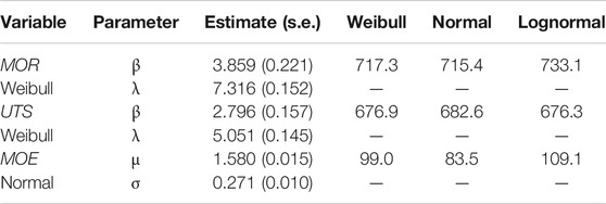
TABLE 2. The parameter estimates and standard errors for the fitted Weibull distributions for MOR, UTS, and fitted normal distribution for MOE. The Weibull density parametrization being used is $f_{\text{Weibull}}\left(x;\beta ,\lambda \right)=\beta {\lambda }^{-1}{\left(x/\lambda \right)}^{\beta -1}\text{exp}\left[-{\left(x/\lambda \right)}^{\beta }\right]$ for x>0. The AIC values for the fitted Weibull, log-normal, and normal distributions are on the right-hand side.

Based on exploratory analysis and diagnostic quantile-quantile plots together with extreme value theory, we choose to use Weibull distributions for MOR and UTS, and the normal distribution for the MOE, as the univariate step before fitting copula models. The Weibull distribution is one of the limiting distributions of the minimum of a sequence of weakly dependent random variables. This fact often justifies the use of the Weibull distribution for modeling the failure strength resulting from the weakest link. On the other hand, the normal distribution is a reasonable model for the elastic properties since the overall elasticity of a specimen depends on the average elasticity over different segments of the lumber. With these choices for the three variables, the resulting maximum likelihood estimates with standard errors for the model parameters are summarized in Table 2.

3 Copula-Based Dependency Analysis

In this section, we use a copula-based method to estimate the dependence among the three lumber strength variables MOR, UTS, and MOE. More specifically, the R100 and T100 groups are used to estimate the bivariate distributions (MOR, MOE) and (UTS, MOE). The R20 and T20 groups are used to estimate the conditional bivariate distribution of (MOR, UTS) given MOE, and then this combination of the two preceding bivariate distributions leads to the trivariate distribution of (MOR, UTS, MOE). The R40/R60/T40/T60 groups are used to assess the fits of different trivariate models. A brief introduction to the notion of copula is included in Section 3.1 before analyses are presented in Sections 3.2 and 3.3.

3.1 Brief Introduction to Copulas for Dependence Modeling

From Ref. [13], for a d-variate distribution F with univariate margins F₁$,\dots ,$F_d, the copula associated with F is a distribution function C:[0,1]^d$\to$[0, 1] with uniform (0,1) margin that satisfies

$F\left(\mathit{x}\right)=C\left[F_1\left(x_1\right),\dots ,F_d\left(x_d\right)\right],\hspace{0.17em}\mathit{x}\in {\mathrm{ℝ}}^d.(1)$

If F is a continuous d-variate distribution function with univariate margins F₁$,\dots ,$F_d and quantile functions F₁⁻¹$,\dots ,$F⁻¹_d, then

$C\left(\mathit{u}\right)=F\left[F_1^{-1}\left(u_1\right),\dots ,F^{-1}\left(u_d\right)\right],\hspace{0.17em}\mathit{u}\in {\left[\mathrm{0,1}\right]}^d,$

is the unique choice. If F₁$,\dots ,$F_d are absolutely continuous with densities f₁$,\dots ,$f_d, respectively, the joint density from differentiating Eq. 1 is

$f\left(\mathit{x}\right)=c\left[F_1\left(x_1\right),\dots ,F_d\left(x_d\right)\right]\hspace{0.17em}{f}_1\left(x_1\right)\cdots f_d\left(x_d\right),(2)$

where $c\left(\mathit{u}\right)={\partial }^{d}C\left(\mathit{u}\right)/\partial u_1\cdots \partial u_d$.

Copula models are useful for dependence analysis because F₁$,\dots ,$F_d can be arbitrary univariate margins, chosen separately from the dependence structure represented by the copula C. For statistical analysis, parametric univariate models are fitted for F₁$,\dots ,$F_d, followed by parametric models for C. Please refer to Ref. [14] for a more detailed introduction to copula theory, models, and applications.

3.2 Copula-Based Model Analysis for Three Strength Variables

For simpler notation, let X = MOR, Y = UTS, and Z = MOE, with realized values x_i,y_i,z_i if these are observed for specimen i in an experimental group. The proposed analysis on the lumber data set based on the copula method is outlined below.

1 For group R100: Observed data are (z_i,x_i). We fit a bivariate copula model for MOE and MOR to estimate the dependence between x and z based on the copula likelihood function.

2 For group T100: Observed data are (z_i,y_i). We fit a bivariate copula model for MOE and UTS to estimate the dependence between y and z based on the copula likelihood function.

3 For group R20/40/60: Observed data are (z_i,x_i) for x_i below the 20/40/60^th-percentile threshold x^(20/40/60), or (z_i,x^(20/40/60),y_i^*) otherwise, where y_i^* is a weakened measure of UTS after proof loading in the rupture mode.

4 For group T20/40/60: Observed data are (z_i,y_i) for y_i below the 20/40/60^th-percentile threshold y^(20/40/60), or (z_i,y^(20/40/60),x_i^*) otherwise, where x_i^* is a weakened measure of MOR after proof loading in the tension mode.

5 For the combination of the R20 and T20 groups, we estimate a parameter for the conditional dependence of MOR and UTS given MOE.

3.3 Analysis Assuming No Damage due to Proof Loading

To simplify the analysis, we first assume that there is no damage or weakening in the proof loading procedure for the R20/T20 groups. That is, for group R20, y_i^*=y_i for all i for the lumber specimens that survive the bending mode. Similarly, for group T20, x_i^*=x_i for the lumber specimens that survive the tension mode. In making reference to cumulative damage theory, Ref. [15] suggests that a very small percentage will be weakened and that residual strength is virtually equal to original strength. In Section 4, a graphical method is used to assess the validity of the “no weakening” assumption for the R20/T20 groups.

3.3.1 Bivariate Analysis for (MOE, MOR) and (MOE, UTS)

We analyze the dependence between the bivariate observations based on groups R100 and T100. To decide whether non-Gaussian copulas might be required, deviations for bivariate Gaussian dependence can be assessed after variables have been (rank) transformed to N (0, 1). Non-Gaussian dependence would be relevant if the scatterplot is far from the elliptical shape, with tail asymmetry or sharper corners (Section 1.4 of Ref. [14]). In addition, sample semi-correlations ${\widehat{\rho }}_N^{-},{\widehat{\rho }}_N^{+}$ can be computed from the points in the lower quadrant and upper quadrant, respectively, to get an assessment of tail asymmetry (more dependence in one joint tail than another). For a variable with n observations, if the ith order statistic is rank transformed to $\frac{i-1/2}{n}$, then ${\Phi }^{-1}\left(\frac{i-1/2}{n}\right)$ is the normal score for that variable, where $\Phi$ is the cumulative distribution function (CDF) of the standard normal random variable. The scatterplot and normal scores plot of (MOE, MOR) based on R100 and the plots of (MOE, UTS) based on T100 are shown in Figures 1 and 2, respectively. From the plots, it can be seen that both pairs of observations have strong dependence. In addition, the correlations and semi-correlations of the normal scores for R100 and T100 are given in Table 3. The semi-correlations indicate slight asymmetric dependence in the joint tails for both groups. These diagnostics suggest that, for two bivariate margins, we can use Gaussian copulas or parametric families of copulas that deviate a little from Gaussian.

FIGURE 1

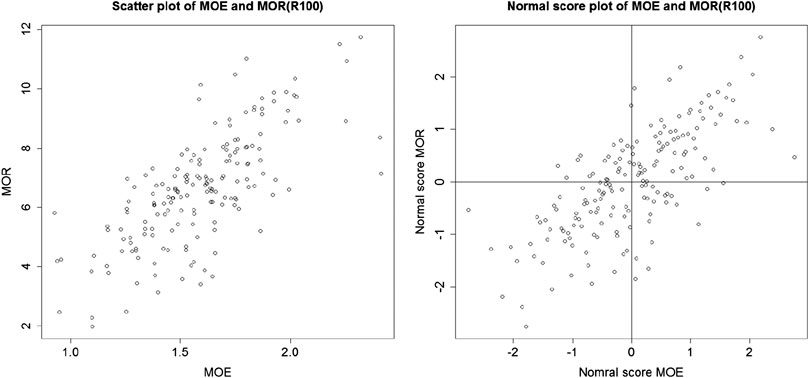
FIGURE 1. Left: scatterplot of (MOE, MOR) based on R100. Right: normal scores plot of (MOE, MOR) based on R100.

FIGURE 2

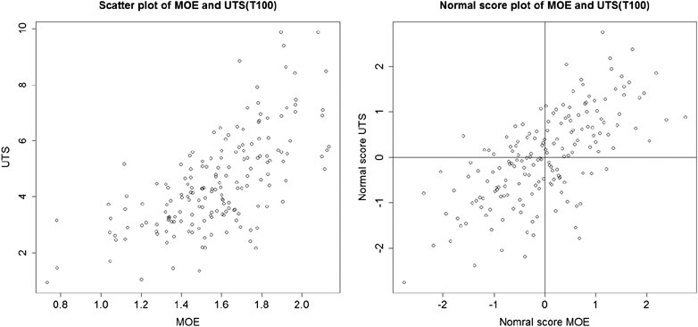
FIGURE 2. Left: scatterplot of (MOE, UTS) based on T100. Right: normal scores plot of (MOE, UTS) based on T100.

TABLE 3

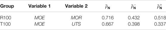
TABLE 3. The correlation and semi-correlations of the normal scores for R100 and T100. ${\widehat{\rho }}_N$ denotes the correlation of normal scores. The semi-correlations ${\widehat{\rho }}_N^{-}$ and ${\widehat{\rho }}_N^{+}$ denote the correlations in the lower quadrant and upper quadrant, respectively, in the right-hand side of Figures 1 and 2.

Let the joint distribution of (MOR, UTS, MOE) be

$F\left(x,y,z;\mathit{\eta },\mathit{\delta }\right)=C\left[F_1\left(x;{\mathit{\eta }}_1\right),F_2\left(y;{\mathit{\eta }}_2\right),F_3\left(z;{\mathit{\eta }}_3\right);\mathit{\delta }\right],$

where $\mathit{\delta }$ is the vector of dependence parameters. F₁,F₂,F₃ are the univariate CDF’s of MOR, UTS, MOE, respectively, with corresponding densities f₁,f₂,f₃ and parameter vectors ${\mathit{\eta }}_1,{\mathit{\eta }}_2,{\mathit{\eta }}_3$, and $\mathit{\eta }=\left({\mathit{\eta }}_1,{\mathit{\eta }}_2,{\mathit{\eta }}_3\right)$. Let F₁₂,F₁₃,F₂₃ be the bivariate marginal CDF’s with respective copula CDF’s C₁₂,C₁₃,C₂₃ and copula densities c₁₂,c₁₃,c₂₃. From Eq. 2 applied to bivariate margins, the log-likelihood functions for the R100 group and T100 groups are as follows, respectively:

$L_{R100}=\underset{i}{{\displaystyle {\displaystyle \sum _i\left\{\log c_{13}\left[F_1\left(x_i;{\mathit{\eta }}_1\right),F_3\left(z_i;{\mathit{\eta }}_3\right);{\delta }_{13}\right]+\text{log}\left[f_1\left(x_i;{\mathit{\eta }}_1\right)\right]+\text{log}\left[f_3\left(z_i;{\mathit{\eta }}_3\right)\right]\right\}}}},(3)$

$L_{T100}={\displaystyle \sum }_i\left\{\log c_{23}\left[F_2\left(y_i;{\mathit{\eta }}_2\right),F_3\left(z_i;{\mathit{\eta }}_3\right);{\delta }_{23}\right]+\text{log}\left[f_2\left(y_i;{\mathit{\eta }}_2\right)\right]+\text{log}\left[f_3\left(z_i;{\mathit{\eta }}_3\right)\right]\right\},(4)$

where ${\delta }_{13},{\delta }_{23}$ are the dependence parameters for the (1,3) and (2,3) margins, respectively. These likelihood functions measure the support provided by the data for possible values of the corresponding parameter vectors.

For multivariate analysis with copula models, it is common to use a two-stage estimation method to assess the adequacy of the univariate and copula models, since the dependence modeled through the copula is separated from the univariate margins. The first stage finds good fitting parametric models for univariate margins, and the second stage fixes the univariate parameters and estimates copula parameters by maximizing the log-likelihood. The two-stage estimation method is statistically efficient unless there is very strong dependence. In addition, the two-stage estimation approach is also a convenient way to compare different copula models and is less sensitive to copula model misspecification. Please refer to Section 1.5.2 of Ref. [14] for details of the two-stage estimation method.

With the two-stage estimation method, we fix the univariate parameters as in Table 2 and consider a few parametric bivariate copula models for R100 and T100 data. Chapter 4 of Ref. [14] has densities and properties of the parametric copula families that we fit. We only consider a few copula families which differ a little from Gaussian; these are summarized next.

•The bivariate t(ν) copula is similar to bivariate Gaussian except it has more dependence in the joint tails as v>0 decreases.

•The bivariate Frank copula has similar properties to bivariate Gaussian but has less dependence in the joint tails than Gaussian.

•The bivariate Gumbel copula has more dependence in the joint upper tail than joint lower tail, and reflected Gumbel satisfies the converse. If V₁,V₂ are U (0, 1) random variables such that (V₁,V₂)∼C₁₂, then the reflected copula of C₁₂ is the distribution of the reflected pair $\left(1-V_1,1-V_2\right)$ leading to $C_{12,\text{reflected}}\left(v_1,v_2\right)=v_1+v_2-1+C_{12}\left(1-v_1,1-v_2\right)$.

The log-likelihood and AIC values based on the copula families are given in Table 4. The different families provide similar fits, and the more tail asymmetric copulas (Gumbel and reflected Gumbel) fit less well. Based on the AIC values and the bivariate scatterplots, there are not much improvements on the bivariate Gaussian copulas, so for simplicity of interpretation, we consider Gaussian copula to be adequate for both R100 and T100. In the next subsection, we consider the trivariate copula with an additional bivariate copula for the conditional dependence of MOR, UTS given MOE.

TABLE 4

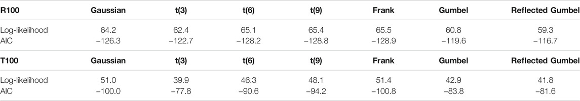
TABLE 4. Model comparison for groups R100 and T100: the log-likelihood and AIC values based on different parametric copula models with fixed univariate parameters/distributions. The notation t(ν) indicates the bivariate t copula with degree of freedom parameter ν.

3.3.2 Trivariate Analysis on MOE, MOR, and UTS with the Vine Copula

In this section, we analyze the dependence among the trivariate observations MOE, MOR, and UTS. Assuming a vine structure on three variables as shown in Figure 3, the copula density is

$f_{123}=c_{13}\left(F_1,F_3;{\delta }_{13}\right)\cdot c_{23}\left(F_2,F_3;{\delta }_{23}\right)\cdot c_{12;3}\left(F_{1|3},F_{2|3};{\delta }_{12;3}\right)\cdot \hspace{0.17em}{f}_1{f}_2{f}_3,(5)$

where ${\delta }_{13},{\delta }_{23},{\delta }_{12;3}$ are the dependence parameters associated with the bivariate copula densities c₁₂,c₁₃,c_12;3. The copula density c_12;3 is used for the conditional dependence of MOR and UTS given MOE. This vine structure follows naturally from the experimental design. The two pairs or edges XZ and YZ in tree T₁ are the two pairs of bivariate variables observed in groups R100 and T100, and the edge XY;Z in tree T₂ allows us to estimate the conditional dependence between X = MOR and Y = UTS, which cannot be simultaneously observed, given Z = MOE. Please refer to Refs. 14,16,17 and 18 for more information about vines and vine copulas, and their derivations.

FIGURE 3

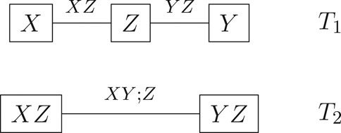
FIGURE 3. A vine structure on three variables with two trees: X = MOR, Y = UTS, and Z = MOE.

The vine copula is an approach to construct a multivariate copula with flexible dependence. There is no general method to construct a multivariate copula from the set of bivariate marginal copulas, and the vine construction approach avoids compatibility issues for $d\ge 3$ variables by using d−1 bivariate marginal copulas and $\left(d-1\right)\left(d-2\right)/2$ bivariate copulas to represent conditional dependence based on 1,2$,\dots ,$ or d−2 variables. In our context, the conditioning on MOE is natural and we are illustrating the simplest vine copula with one edge representing bivariate conditional dependence.

For the groups with proof loading, a complication is a likelihood function with censored data. Take the group R20 as an example. Let $K_1=\left\{i:\left(z_i,x_i\right)\text{observed}\right\}$, and $K_2=\left\{j:\left(z_j,x^{\left(20\right)},y_j\right)\text{observed}\right\}$. Let

$F_{1|23}\left(x|y,z;\mathit{\eta },\mathit{\delta }\right)=C_{1|2;3}\left[F_{1|3}\left(x|z;{\mathit{\eta }}_1,{\mathit{\eta }}_3,{\delta }_{13}\right)|F_{2|3}\left(y|z;{\mathit{\eta }}_2,{\mathit{\eta }}_3,{\delta }_{23}\right);{\delta }_{12;3}\right],$

where $C_{1|2;3}(\cdot )$ is a conditional distribution (partial derivative with respect to the second argument) of the bivariate copula C_12;3(⋅). The log-likelihood function for the R20 group is

$\begin{array}{c}{L}_{R20}={\displaystyle \sum }_{i\in K_1}\left\{\log c_{13}\left[F_1\left(x_i;{\mathit{\eta }}_1\right),F_3\left(z_i;{\mathit{\eta }}_3\right);{\delta }_{13}\right]+\text{log}\left[f_1\left(x_i;{\mathit{\eta }}_1\right)\right]+\text{log}\left[f_3\left(z_i;{\mathit{\eta }}_3\right)\right]\right\}\\ \hspace{0.17em}+{\displaystyle \sum }_{j\in K_2}\{\log {\overline{F}}_{1|23}\left(x^{\left(20\right)}|y_j,z_j;\mathit{\eta },\mathit{\delta }\right)+\text{log}{c}_{23}\left[F_2\left(y_j;{\mathit{\eta }}_2\right),F_3\left(z_j;{\mathit{\eta }}_3\right);{\delta }_{23}\right]\\ \hspace{0.17em}+\text{log}\left[f_2\left(y_j;{\mathit{\eta }}_2\right)\right]+\text{log}\left[f_3\left(z_j;{\mathit{\eta }}_3\right)\right]\},\end{array}(6)$

where ${\overline{F}}_{1|23}(\cdot )=1-F_{1|23}(\cdot )$ is the survival function of $F_{1|23}(\cdot )$ and y_j=y^*_j is assumed for $j\in K_2$. Note that we assume y_j=y^*_j because in this section we are performing estimation assuming no damage during proof loading.

Similarly, for group T20, let $K_1^{\prime }=\left\{i:\left(z_i,y_i\right)\text{observed}\right\}$ and $K_2^{\prime }=\left\{j:\left(z_j,y^{\left(20\right)},x_j\right)\text{observed}\right\}$. Let

$F_{2|13}\left(y|x,z;\mathit{\eta },\mathit{\delta }\right)=C_{2|1;3}\left[F_{2|3}\left(y|z;{\mathit{\eta }}_2,{\mathit{\eta }}_3,{\delta }_{23}\right)|F_{1|3}\left(x|z;{\mathit{\eta }}_1,{\mathit{\eta }}_3,{\delta }_{13}\right);{\delta }_{12;3}\right],$

where C_21;3(·) is a conditional distribution (partial derivative with respect to the first argument) of the bivariate copula C_12;3(·). The log-likelihood function for the T20 group is

$\begin{array}{c}{L}_{T20}={\displaystyle \sum }_{i\in K_1^{\mathrm{\prime }}}\left\{\log c_{23}\left[F_2\left(y_i;{\mathit{\eta }}_2\right),F_3\left(z_i;{\mathit{\eta }}_3\right);{\delta }_{23}\right]+\text{log}\left[f_2\left(y_i;{\mathit{\eta }}_2\right)\right]+\text{log}\left[f_3\left(z_i;{\mathit{\eta }}_3\right)\right]\right\}\\ \hspace{0.17em}+{\displaystyle \sum }_{j\in K_2^{\mathrm{\prime }}}\{\log {\overline{F}}_{2|13}\left(y^{\left(20\right)}|x_j,z_j;\mathit{\eta },\mathit{\delta }\right)+\log c_{13}\left[F_1\left(x_j;{\mathit{\eta }}_1\right),F_3\left(z_j;{\mathit{\eta }}_3\right);{\delta }_{13}\right]\\ \hspace{0.17em}+\text{log}\left[f_1\left(x_j;{\mathit{\eta }}_1\right)\right]+\text{log}\left[f_3\left(z_j;{\mathit{\eta }}_3\right)\right]\},\end{array}(7)$

where ${\overline{F}}_{2|13}(\cdot )=1-F_{2|13}(\cdot )$ is the survival function of $F_{2|13}(\cdot )$ and x_j=x_j^*is assumed for$j\in K_2^{\mathrm{\prime }}$. To estimate the conditional dependence parameter${\delta }_{12;3}$ofC_12;3, we create a log-likelihood function from the sum of Eqs 6 and 7.

For proof loading to the 40^th and 60^th percentiles, it might be more likely that there is some weakening or damage to the surviving lumber specimens so that the R40/R60/T40/T60 groups are not included in the above log-likelihoods.

To summarize, the sequential steps are as follows in order that model comparisons can be done at each stage based on the estimated marginal models of previous stages.

• $L_1\left({\mathit{\eta }}_1\right)$ is the log-likelihood based on a density $f_1\left(\cdot ;{\mathit{\eta }}_1\right)$ for MOR from the R100 data.

• $L_2\left({\mathit{\eta }}_2\right)$ is the log-likelihood based on a density $f_2\left(\cdot ;{\mathit{\eta }}_2\right)$ for UTS from the T100 data.

• $L_3\left({\mathit{\eta }}_3\right)$ is the log-likelihood based on a density $f_3\left(\cdot ;{\mathit{\eta }}_3\right)$ for MOE from the R100 and T100 data.

• $L_{13}\left({\delta }_{13}\right)=L_{13}\left({\delta }_{13};{\widehat{\mathit{\eta }}}_1,{\widehat{\mathit{\eta }}}_3\right)$, from Eq. 3, is the log-likelihood based on a density $c_{13}\left(\cdot ;{\delta }_{13}\right)$ for MOR, MOE from the R100 data, with estimated univariate parameters.

• $L_{23}\left({\delta }_{23}\right)=L_{13}\left({\delta }_{13};{\widehat{\mathit{\eta }}}_2,{\widehat{\mathit{\eta }}}_3\right)$, from Eq. 4, is the log-likelihood based on a density $c_{23}\left(\cdot ;{\delta }_{23}\right)$ for UTS, MOE from the T100 data, with estimated univariate parameters.

• $L_{12;3}\left({\delta }_{12;3}\right)=L_{12;3}\left({\delta }_{12;3};{\widehat{\mathit{\eta }}}_1,{\widehat{\mathit{\eta }}}_2,{\widehat{\mathit{\eta }}}_3,{\widehat{\delta }}_{13},{\widehat{\delta }}_{23}\right)$, from the sum of Eqs 6 and 7, is the log-likelihood based on a copula $C_{12;3}\left(\cdot ;{\delta }_{12;3}\right)$ for the conditional dependence of MOR, UTS given MOE from the R20/T20 data, with estimated univariate parameters and estimated bivariate dependence parameters for each of MOR, UTS paired with MOE.

If MOR, UTS, and MOE follow a trivariate Gaussian copula, the parametrization involves a partial correlation of transformed MOR, UTS given MOE to represent the conditional dependence. Note that for a given correlation matrix R of dimension d×d, the multivariate Gaussian copula is defined as

$C\left(\mathit{u},\mathit{R}\right)={\Phi }_d\left[{\Phi }^{-1}\left(u_1\right),{\Phi }^{-1}\left(u_2\right),\dots ,{\Phi }^{-1}\left(u_d\right);\mathit{R}\right],\hspace{0.17em}\mathit{u}\in {\left[\mathrm{0,1}\right]}^d,$

when R is positive definite, where $\Phi$ denotes the univariate standard Gaussian distribution function and ${\Phi }_d$ denotes the joint CDF of a multivariate normal distribution with mean vector 0 and covariance matrix equal to the correlation matrix R.

When d=3, R can be written as

$R=\left[\begin{array}{ccc}1& {\rho }_{12}& {\rho }_{13}\\ {\rho }_{12}& 1& {\rho }_{23}\\ {\rho }_{13}& {\rho }_{23}& 1\end{array}\right].$

To avoid the positive definite matrix constraint, we define the partial correlation

${\rho }_{12;3}=\left({\rho }_{12}-{\rho }_{13}{\rho }_{23}\right)\mathrm{/}\sqrt{\left(1-{\rho }_{13}^2\right)\left(1-{\rho }_{23}^2\right)}$

or equivalently ${\rho }_{12}={\rho }_{13}{\rho }_{23}+{\rho }_{12;3}\sqrt{\left(1-{\rho }_{13}^2\right)\left(1-{\rho }_{23}^2\right)}\hspace{0.17em}$. Then the correlation matrix can be parameterized by $\left({\rho }_{13},{\rho }_{23};{\rho }_{12;3}\right)$, and these parameters are algebraically independent on the cube (−1,1)³. That is, the vector $\left({\rho }_{13},{\rho }_{23};{\rho }_{12;3}\right)$ is free to vary in (−1,1)³, and the resulting correlation matrix R is always positive definite.

Under the trivariate Gaussian copula setting, c₁₃, c₂₃, c_12;3, $c_{23}$, and $c_{12;3}$ in Eq. 5 can be written as

$\begin{array}{l}{c}_{13}\left(u,v,{\rho }_{13}\right)=c_{\text{Gaussian}}\left(u,v,{\rho }_{13}\right),\\ c_{23}\left(u,v,{\rho }_{23}\right)=c_{\text{Gaussian}}\left(u,v,{\rho }_{23}\right),\\ c_{12;3}\left(u,v,{\rho }_{12;3}\right)=c_{\text{Gaussian}}\left(u,v,{\rho }_{12;3}\right),\end{array}$

where

$c_{\text{Gaussian}}\left(u,v,\rho \right)=\frac{\text{exp}\langle -\frac{1}{2}\left\{{\left[{\Phi }^{-1}\left(u\right)\right]}^2+{\left[{\Phi }^{-1}\left(v\right)\right]}^2-2\rho \hspace{0.17em}{\Phi }^{-1}\left(u\right)\hspace{0.17em}{\Phi }^{-1}\left(v\right)\right\}/(1-{\rho }^2)\rangle }{\sqrt{1-{\rho }^2}\text{exp}\langle -\frac{1}{2}\left\{{\left[{\Phi }^{-1}\left(u\right)\right]}^2+{\left[{\Phi }^{-1}\left(v\right)\right]}^2\right\}\rangle }.$

The general trivariate vine copula is essentially an extension of the trivariate Gaussian copula after the latter has been parameterized to $\left({\rho }_{13},{\rho }_{23},{\rho }_{12;3}\right)$. As in Table 4, we can also consider other parametric copula families for C_XY;Z=C_12;3 with the log-likelihood from the sum of Eqs 6 and 7. With the bivariate copula families summarized in Section 3.3.1, the results are summarized in Table 5.

TABLE 5

TABLE 5. Model comparison based on the sum of Eqs 6 and 7 for groups R20/T20: the log-likelihood and AIC values based on different parametric copula models for C_12;3 to represent the conditional dependence of (MOR, UTS) given MOE, with fixed univariate models and fixed bivariate Gaussian copulas C₁₃ for (MOR, MOE) and C₂₃ for (UTS, MOE). The notation t(ν) indicates the bivariate t copula with degree of freedom parameter ν.

No other copula family for C_12;3 is substantially better than Gaussian, so it is simpler to next proceed with the assessment of the fit of the trivariate Gaussian copula. Note that the graphical method for assessing damage introduced in Section 4 is mostly not sensitive to the choices of the bivariate copulas in the vine. Different bivariate copulas lead to similar conclusions when using the proposed graphical method to assess the damage effect of proof loading. The parameter estimates (and corresponding conditional standard errors) for this trivariate Gaussian copula are

${\rho }_{13}=0.726\hspace{0.17em}\left(0.029\right),\hspace{1em}{\rho }_{23}=0.678\hspace{0.17em}\left(0.034\right),\hspace{1em}{\rho }_{12;3}=0.587\hspace{0.17em}\left(0.142\right),\hspace{1em}{\rho }_{12}=0.789\hspace{0.17em}\left(0.072\right).(8)$

The standard errors are based on the square root of inverse of the second derivative of the negative log-likelihoods corresponding to L₁₃,L₂₃,L_12;3 as mentioned above. Not surprisingly, ${\rho }_{12;3}$ is estimated with much less precision because of the censoring and the fact that MOR and UTS cannot be measured simultaneously. It can be seen from the profile negative log-likelihoods in Figure 4 that $L_{12;3}\left({\rho }_{12;3}\right)$ is much flatter near the optimal value. Reference [8] uses a trivariate normal copula with log-normal univariate margins and has similar estimates of the pairwise correlations of the strength measurements. Using a regression approach and proof loading experiments with different upper bound loads, Ref. [5] has some point estimates of correlation of MOR and MOE exceeding 0.9, but with wide interval estimates.

FIGURE 4

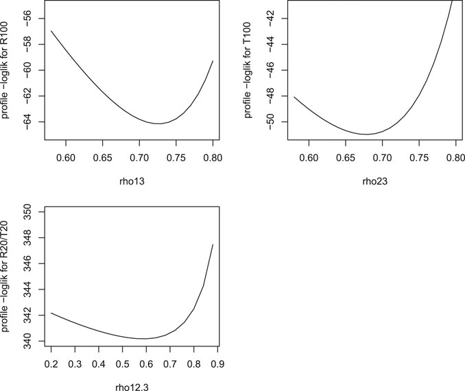
FIGURE 4. Plots of profile negative log-likelihoods for $L_{13}\left({\rho }_{13}\right),L_{23}\left({\rho }_{23}\right),L_{12;3}\left({\rho }_{12;3}\right)$.

4 Graphical Method to Assess the Damage Effect of Proof Loading

In this section, we take the possible weakening due to proof loading into consideration and suggest a graphical method, using Q-Q plots and simulated data from the fitted model, to examine the empirical damage effect and assess the assumptions used in Section 3.3. The details of the graphical method are given in Section 4.1. In Section 3, the parameter estimates and copula family candidates are based on the groups R100, T100, R20, and T20; the additional groups R40, R60, T40, and T60 are used for sensitivity analysis of copula choice and an assessment of the damage effect of proof loading. This topic is not covered in the other experiments reported in Section 2. Further analyses are given in Section 4.2.

4.1 Assessing the Damage Effect

In Section 3, we analyze the lumber data by assuming there is no weakening due to proof loading. But this assumption may not hold for all the experimental groups, especially for R40 and T40, where the level is relatively higher. We propose a graphical method based on the Q-Q plot to evaluate whether the estimated dependence parameters represent the damage effect well enough. Take the group R20 as an example. We can compare the following two sets of data.

a. Simulated distribution, with sample size n, for UTS given MOR is greater than its 20^th quantile, based on the fitted trivariate model and its estimated univariate and dependence parameters.

b. Observed distribution of residual UTS (i.e., Y^*) given observed MOR is greater than its 20^th quantile.

The trivariate distribution of X, Y, and Z is such that the values of a) should be stochastically larger than those of b), conditioning on MOE in different quantile intervals. That is, if the dependence parameters can accurately represent the damage effect, then in the Q-Q plot of b) against a), we expect to see some or most of the points below the 45^o diagonal line. More points below the diagonal line would be a sign of more weakening. Similar comments hold for the Q-Q plots based on the other proof loaded groups.

We simulated 10,000 sets of trivariate observations of MOR, UTS, and MOE based on the MLE’s in Eq. 8, and the above-mentioned Q-Q plots are shown in Figures 5–10 for groups R20/40/60 and T20/40/60, respectively.

FIGURE 5

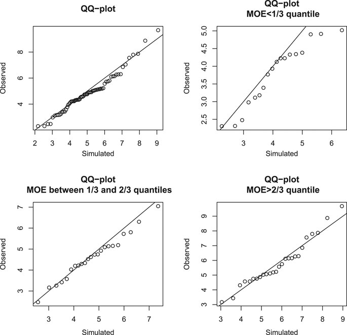
FIGURE 5. Gaussian copula model and R20. Q-Q plot of observed residual UTS against simulated UTS with the identity line, given MOR greater than its 20^th quantile and MOE in different quantile intervals.

FIGURE 6

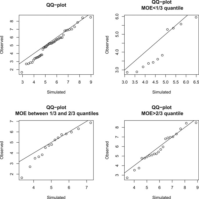
FIGURE 6. Gaussian copula model and R40. Q-Q plot of observed residual UTS against simulated UTS with the identity line, given MOR greater than its 40^th quantile and MOE in different quantile intervals.

FIGURE 7

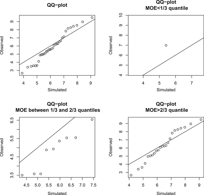
FIGURE 7. Gaussian copula model and R60. Q-Q plot of observed residual UTS against simulated UTS with the identity line, given MOR greater than its 60^th quantile and MOE in different quantile intervals.

FIGURE 8

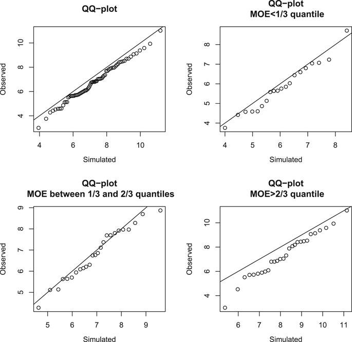
FIGURE 8. Gaussian copula model and T20. Q-Q plot of observed residual MOR against simulated MOR with the identity line, given UTS greater than its 20^th quantile and MOE in different quantile intervals.

FIGURE 9

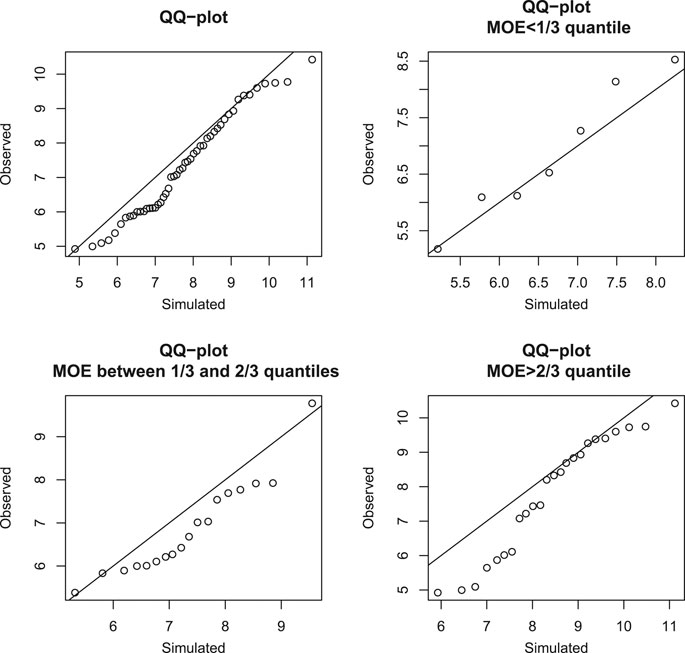
FIGURE 9. Gaussian copula model and T40. Q-Q plot of observed residual MOR against simulated MOR with the identity line, given UTS greater than its 40^th quantile and MOE in different quantile intervals.

FIGURE 10

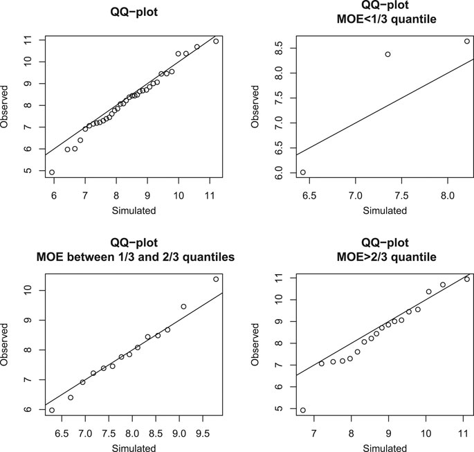
FIGURE 10. Gaussian copula model and T60. Q-Q plot of observed residual MOR against simulated MOR with the identity line, given UTS greater than its 60^th quantile and MOE in different quantile intervals.

It can be seen that, for most groups, points in the Q-Q plots are mainly below or near the diagonal identity line; this indicates that the Gaussian copula model may be fine as a first-order model. For the R20 and T20 groups, the points are mainly marginally below the diagonal line. For the R40 and T40 groups, the points are noticeably mostly below the diagonal line, indicating that there is some weakening of many specimens that survive to the 40^th percentile. For the R60 group, the points are mostly below the diagonal line for the bottom half of those that survive in the rupture mode to the 60^th percentile. However, for the T60 group, the points are fairly close to the diagonal, indicating that the strong specimens that can survive in the tension mode to the 60^th percentile were not weakened. These Q-Q plots have similar patterns even if ${\rho }_{12;3}$ is increased from 0.589 to 0.800 for the simulated distribution.

As a sensitivity analysis to the bivariate copula choices in the vine, the above procedure was applied to other vine copulas mentioned in Section 3. The conclusions are the same for vine copulas that are shown to fit well based on the proposed Q-Q plots. In a case, such as bivariate Gaussian copulas for (MOR, MOE) and (UTS, MOE) and Gumbel copula for the conditional dependence given MOE, the Q-Q plots based on the vine model with these bivariate copulas indicate that this model is not as appropriate because points tended to deviate further below and above the 45^o diagonal line.

4.2 Further Analyses for the Damage Effect

In this subsection, we summarize further analyses to understand the accuracy of estimating the conditional dependence parameter.

i. We simulated R100/T100/R20/T20 data sets with the same sample sizes as in the experiment, assuming the trivariate distribution with Gaussian copula having the parameters in Eq. 8 and Table 2, as well as another parameter set with ${\rho }_{12;3}=0.800$$\left({\rho }_{12}=0.899\right)$ but other bivariate and univariate parameters unchanged. With 100 replications in each case, we find that the MLEs of the parameters each have minimal bias, but the estimate of ${\rho }_{12;3}$ has the largest root mean square error among dependence parameters (0.17 with true ${\rho }_{12;3}=0.587$, and 0.08 with true ${\rho }_{12;3}=0.800$, whereas the root mean square error is 0.04 for estimates of ${\rho }_{13}$ and ${\rho }_{23}$).

ii. We simulated data sets as i) with parameters in Eq. 8 and Table 2. But for the R20/T20, we multiplied the UTS and MOR values of surviving specimens after proof loading by a number less than 1. With more “damage,” we find more negative bias (and increased SD) for the estimated ${\rho }_{12;3}$ parameter. For example, for no damage, the bias is in −0.01 with a SD of 0.17; for x_i^*=ax_i and y_i^*=ay_i with a uniform in (0.97,1), the bias is −0.10 with a SD of 0.18; for x_i^*=ax_i and y_i^*=ay_i with a = 0.97, the bias is −0.15 with a SD of 0.25.

iii. For the surviving specimens in the actual experimental R20 and T20 groups, we assume that $y_i=1.1y_i^{\text{*}}$ (for R20) and x_i=1.1x_i^* (for T20) for the purpose of another maximum likelihood evaluation in the sum of Eqs 6 and 7. This corresponds to the approximation that the actual strength measurements are 1.1 times the observed weakened measurements. The maximum likelihood estimate of ${\rho }_{12;3}$ increases to 0.747. If 1.05 is used in place of 1.1, the maximum likelihood estimate of ${\rho }_{12;3}$ increases only to 0.693.

iv. The vine copula approach is flexible enough so that the strength of conditional dependence can vary with the conditioning values (of MOE in the current application). Similar to examples in Ref. [19], we can modify Eqs 6 and 7 with bivariate Gaussian copulas so that C_12;3 has parameter ${\rho }_{12;3}\left(z\right)$ that depends on the value of MOE. Using variations of $\text{log}\left\{{\rho }_{12;3}\left(z\right)/\left[1-{\rho }_{12;3}\left(z\right)\right]\right\}$ or ${\rho }_{12;3}\left(z\right)$ as linear functions of a transform of F₃(z), the log-likelihood with one extra regression parameter increased from −340.2 to −339.4; the regression parameter was always negative suggesting that the conditional dependence is decreasing as the value of MOE increases. But this effect is not significant based on standard errors. For example, with $\text{log}\left\{{\rho }_{12;3}\left(z\right)/\left[1-{\rho }_{12;3}\left(z\right)\right]\right\}={\beta }_0+{\beta }_1{F}_3\left(z\right)$, the vector $\left({\beta }_0,{\beta }_1\right)$ is estimated as (1.17, 2.81) so that ${\rho }_{12;3}$ decreases from 0.77 to 0.16 as F₃(z) increases from 0 to 1.

The above extra analyses suggest that the assumption of no weakening or damage in the R20/T20 survivors might lead to an underestimation of the parameter representing conditional dependence of MOR and UTS given MOE. Furthermore, there is the possibility that the conditional dependence is not constant over values of MOE.

5 Conclusion

The proof loading experiment discussed in this article allows for modeling and estimation of the conditional dependence of MOR and UTS given MOE, in addition to bivariate dependence parameters for (MOR, MOE) and (UTS, MOE) and univariate marginal parameters. From model fitting and diagnostics, we conclude that there is a strong dependence between MOR and UTS when conditioning on MOE. Our analysis takes a copula-based multivariate approach with univariate distributions that can be different and a dependence structure, that is, summarized via copulas. We also consider the possible weakening or damage of lumber specimens in the proof loading stage. In earlier research, Ref. [8] assumed a multivariate normal distribution after log transforms of the strength measurements and they did not consider possible damage in the proof loaded group that survived the first stage. Other than these differences, our estimates of the pairwise correlations are comparable when considering the standard errors. A graphical method is used to assess the possible damage effect, and it suggests that there is damage to specimens due to proof loading, especially those specimens that are weaker. The vine copula approach allows for flexible univariate margins and different bivariate copula families to summarize marginal and conditional dependence, and hence this graphical method could be combined with a sensitivity analysis to the model choices in the vine.

With a sample size of 174 for the two shoulder groups of R100 and T100, the univariate parameters and bivariate parameters for (MOR, MOE) and (UTS, MOE) can be well estimated via maximum likelihood. With the sample size of 87 for R20 (bending mode) and T20 (tension mode), because of much censoring, the conditional dependence parameter of MOR and UTS given MOE is not as precisely estimated. With a trivariate Gaussian copula model, the standard error of the conditional dependence parameter ${\widehat{\rho }}_{12;3}$ is approximately 0.15, whereas the standard errors of other bivariate parameters ${\widehat{\rho }}_{13}$ and ${\widehat{\rho }}_{23}$ are about 0.03–0.04. Because the current experiment suggests that there could be some damage or weakening of specimens from first stage proof loading, a future experiment could measure MOE based on traverse vibration for all specimens as well as the survivors of the first stage proof loading (such as R20, R40, R60, T20, T40, and T60). In order to provide a consistent adjustment for moisture content and moisture adjusted MOE, a small fraction of lumber specimens could be set aside and not undergo proof loading in order to measure MOE initially and after other groups have been proof loaded in the first stage. The extra measurements for survivors should help in estimating a joint distribution of MOE, MOR, and UTS.

A better probabilistic model for the dependence among the three lumber strength properties can potentially help reduce the monitoring cost in the lumber industry. Future work could include applying the copula-based method to estimate the dependence among properties of more tree species and lumber sizes and including other strength measurements such as ultimate compression strength in the experimental design. For other methods of strength prediction, see Ref. [20].

Data Availability Statement

The raw data supporting the conclusions of this article will be made available by the authors, without undue reservation.

Author Contributions

YC was involved in the experiment and its planning, did initial univariate and bivariate analyses of the lumber strength properties, and developed theory for the damage of lumber specimens from proof loading. Under the supervision of HJ. SP performed the copula model analysis after YC’s PhD thesis was completed and wrote a draft of most of this paper. HJ completed the writing and additional analyses in Section 4.

Funding

This research has been supported by NSERC Discovery Grant 8698 and a grant to FPInnovations.

Conflict of Interest

The authors declare that the research was conducted in the absence of any commercial or financial relationships that could be construed as a potential conflict of interest.

Acknowledgments

Thanks are due to Professor James V. Zidek and Conroy Lum for feedback and also to the referees for constructive comments leading to an improved presentation.

References

1. Kretschmann, DE. Wood handbook, chapter 05: mechanical properties of wood (2010). p. 5-1–5-46. General Technical Report FPL-GTR-190. Madison, WI: U.S. Department of Agriculture, Forest Service, Forest Products Laboratory.

Google Scholar

2. Kretschmann, DE. Wood handbook, chapter 07: stress grades and design properties for lumber, round timber, and ties (2010). p. 7-1–7-16. General Technical Report FPL-GTR-190. Madison, WI: U.S. Department of Agriculture, Forest Service, Forest Products Laboratory.

Google Scholar

3. Evans, J, Johnson, R, and Green, D. Estimating the correlation between variables under destructive testing, or how to break the same board twice. Technometrics (1984). 26:285–90. doi:10.2307/1267555

CrossRef Full Text | Google Scholar

4. Green, D, Evans, J, and Johnson, R. Investigation of the procedure for estimating concomitance of lumber strength properties. Wood Fiber Sci (1984). 16:427–40.

Google Scholar

5. Johnson, RA, and Galligan, WL. Estimating the concomitance of lumber strength properties. Wood Fiber Sci (1983). 15:235–44.

Google Scholar

6. Johnson, RA, Evans, JW, and Green, DW. “Some bivariate distributions for modeling the strength properties of lumber,”in Research paper FPL-RP-575. Madison, WI: U.S. Department of Agriculture, Forest Service, Forest Products Laboratory (1999).

Google Scholar

7. Verrill, SP, Evans, JW, Kretschmann, DE, and Hatfield, CA. Asymptotically efficient estimation of a bivariate Gaussian-Weibull distribution and an introduction to the associated pseudo-truncated Weibull. Commun Stat Theor Methods (2015). 44:2957–75. doi:10.1080/03610926.2013.805626

CrossRef Full Text | Google Scholar

8. Barnett, NR, and Lwin, T. Estimating a relationship between different destructive tests on timber. Appl Stat (1984). 33:65–72. doi:10.2307/2347664

CrossRef Full Text | Google Scholar

9. Amorim, SD, and Johnson, R. Experimental designs for estimating the correlation between two destructively tested variables. J Am Stat Assoc (1986). 81:807–12. doi:10.1080/01621459.1986.10478338

CrossRef Full Text | Google Scholar

10. Johnson, R, and Lu, W. Proof load designs for estimation of dependence in a bivariate weibull model. Stat Probab Lett (2007). 77:1061–9. doi:10.1016/j.spl.2007.01.002

CrossRef Full Text | Google Scholar

11. Cai, Y. Statistical methods for relating strength properties of dimensional lumber. [PhD thesis]. Vancouver, Canada:University of British Columbia (2015).

Google Scholar

12. Cai, Y, Cai, J, Chen, J, Golchi, S, Guan, M, Karim, ME, et al. An empirical experiment to assess the relationship between the tensile and bending strengths of lumber (2016). Report No.: 276, Vancouver, Canada:Department of Statistics, University of British Columbia.

Google Scholar

13. Sklar, A. Fonctions de répartition à dimensions et leurs marges. Publications de l’Institut de Statistique de l’Université de Paris (1959). Vol. 8, p. 229–31.

Google Scholar

14. Joe, H. Dependence modeling with copulas. Boca Raton, FL: Chapman & Hall/CRC Press (2014).

Google Scholar

15. Steiner, SH, and Wesolowsky, GO. Estimating the correlation between destructively measured variables using proof-loading. Technometrics (1995). 37:94–101. doi:10.1080/00401706.1995.10485892

CrossRef Full Text | Google Scholar

16. Bedford, T, and Cooke, RM. Probability density decomposition for conditionally dependent random variables modeled by vines. Ann Math Artif Intell (2001). 32:245–68. doi:10.1023/A:1016725902970

CrossRef Full Text | Google Scholar

17. Bedford, T, and Cooke, RM. Vines—a new graphical model for dependent random variables. Ann Stat (2002). 30:1031–68. doi:10.1214/aos/1031689016

CrossRef Full Text | Google Scholar

18. Kurowicka, D, and Cooke, R. Uncertainty analysis with high dimensional dependence modelling. Chichester: Wiley (2006).

Google Scholar

19. Chang, B, and Joe, H. Copula diagnostics for asymmetries and conditional dependence. J Appl Stat (2020). 47:1587–615. doi:10.1080/02664763.2019.1685080

CrossRef Full Text | Google Scholar

20. Wong, SWK, Lum, C, Wu, L, and Zidek, JV. Quantifying uncertainty in lumber grading and strength prediction: a Bayesian approach. Technometrics (2016). 58:236–43. doi:10.1080/00401706.2015.1033108

CrossRef Full Text | Google Scholar