Shapley Value Confidence Intervals for Attributing Variance Explained

1. Introduction

When conducting statistical estimation and computation, the assumption of randomness of data necessitates that we address not only the problem of point estimation, but also variability quantification. In Ref. 1, variability for the coefficient of determination Shapley values were quantified via the use of bootstrap confidence intervals (CIs). Combined with the usual computational intensiveness of bootstrap resampling (see, e.g., Refs. 2 and 3; Ch. 12)), the combinatory nature of the computation of Eq. 5 (notice that $\left|\mathcal{P}\right|=d!$) compounds the time complexity of such a method, which is already of order $\mathcal{O}\left(2^d\right)$. In this article, we seek to provide an asymptotic method for computing CIs for the Shapley values.

Our approach uses the joint asymptotic normality result of the elements in a correlation matrix, under an elliptical assumption, via [4], combined with asymptotic normality results concerning the determinants of a correlation matrix, of Refs. 5 and 6. Using these results, we derive the asymptotic joint distribution for the $R^2\left({\mathcal{Ƶ}}_n\right)$ Shapley values, which allows us to construct CIs for each of the values and their contrasts. We assess the finite sample properties of our constructions via a comprehensive Monte Carlo study and demonstrate the use of our CIs via applications to real estate price data.

The remainder of the article proceeds as follows. In Section 3, we present our main results regarding the asymptotic distribution of the coefficient of determination Shapley values, and their CI constructions. In Section 4, we present a comprehensive Monte Carlo study of our CI construction method. In Section 5, we demonstrate how our results can be applied to real estate price data. Conclusions are lastly drawn in Section 6. All data and scripts to reproduce the analyses are available at https://github.com/ex2o/shapley_confidence.

2. Background

2.1. The Coefficient of Determination

The multiple linear regression model (MLR) is among the most commonly applied tools for statistics inference; see Refs. 7 and 8; Part I) for thorough introductions to MLR models. In the usual MLR setting, one observes an independent and identically distributed (IID) sample of data pairs ${\mathit{Z}}_i^{\mathrm{\top }}=\left(Y_i,{\mathit{X}}_i^{\mathrm{\top }}\right)\in {\mathrm{ℝ}}^{d+\text{1}}$, where $i\in \left[n\right]=\left\{1,\dots ,n\right\}$, and $d,n\in \mathrm{\mathbb{N}}$. The MLR model is then defined via the linear relationship

$\left(Y_i|{\mathit{X}}_i={\mathit{x}}_i\right)={\beta }_0+{\displaystyle \sum _{j=1}^d{\beta }_j{X}_{ij}},$

where ${\mathit{\beta }}^{\mathrm{\top }}=\left({\beta }_0,\dots ,{\beta }_n\right)\in {\mathrm{ℝ}}^{d+\text{1}}$, and ${\mathit{X}}_i^{\mathrm{\top }}=\left(X_{i1},\dots ,X_{id}\right)$. We shall also write ${\mathit{Z}}_i^{\mathrm{\top }}=\left(Z_{i0},Z_{i1},\dots ,Z_{id}\right)$, when it is convenient to do so. Here, ${(\cdot )}^{\mathrm{\top }}$ is the transposition operator.

The usual nomenclature is to call the $Y_i$ and ${\mathit{X}}_i$ elements of each pair, the response (or dependent) variable and the explanatory (or covariate) vector, respectively. Here, the jth element of ${\mathit{X}}_i$: $X_{ij}$$\left(j\in \left[d\right]\right)$, is referred to as the $j\text{th}$ explanatory variable (or the $j\text{th}$ covariate). We may put the covariate and response pairs into a dataset ${\mathcal{Ƶ}}_n={\left\{{\mathit{Z}}_i\right\}}_{i=1}^n$.

Let $R_{jk}\left({\mathcal{Ƶ}}_n\right)$ denote the sample correlation coefficient

$R_{jk}\left({\mathcal{Ƶ}}_n\right)=\frac{{{{\displaystyle \sum }}^{\text{}}}_{i=1}^n\left(Z_{ij}-{\overline{Z}}_j\right)\left(Z_{ik}-{\overline{Z}}_k\right)}{\sqrt{{{{\displaystyle \sum }}^{\text{}}}_{i=1}^n{\left(Z_{ij}-{\overline{Z}}_j\right)}^2}\sqrt{{{{\displaystyle \sum }}^{\text{}}}_{i=1}^n{\left(Z_{ik}-{\overline{Z}}_k\right)}^2}},(1)$

for each $j,k\in \left\{0\right\}\cup \left[d\right]$. Here ${\overline{Z}}_j=n^{-1}{{{\displaystyle \sum }}^{\text{}}}_{i=1}^n{Z}_{ij}$ is the sample mean of variable j. Write $\mathcal{U}\subseteq \left\{0\right\}\cup \left[d\right]$ be a nonempty subset, where $\mathcal{U}=\left\{u_1,\dots ,u_{\left|\mathcal{U}\right|}\right\}$, where $\left|\mathcal{U}\right|$ is the cardinality of $\mathcal{U}$. We refer to the matrix of correlations between the variables in $\mathcal{U}$ as

${\mathbf{C}}_n\left(\mathcal{U}\right)=\left[\begin{array}{cccc}1& R_{u_1{u}_2}\left({\mathcal{Ƶ}}_n\right)& \cdots & R_{u_1{u}_{\left|U\right|}}\left({\mathcal{Ƶ}}_n\right)\\ R_{u_2{u}_1}\left({\mathcal{Ƶ}}_n\right)& 1& \cdots & R_{u_2{u}_{\left|\mathcal{U}\right|}}\left({\mathcal{Ƶ}}_n\right)\\ ⋮& ⋮& \ddots & ⋮\\ R_{u_{\left|\mathcal{U}\right|}{u}_1}\left({\mathcal{Ƶ}}_n\right)& R_{u_{\left|\mathcal{U}\right|}{u}_2}\left({\mathcal{Ƶ}}_n\right)& \cdots & 1\end{array}\right].(2)$

A common inferential task is to determine the degree to which the response can be explained by the covariate vector, in totality. The usual device for addressing this question is via the coefficient of determination (or squared coefficient of multiple correlation), which is defined as

$R^2\left({\mathcal{Ƶ}}_n\right)=1-\frac{\left|{\mathbf{C}}_n\left(\left\{0\right\}\cup \left[d\right]\right)\right|}{\left|{\mathbf{C}}_n\left(\left[d\right]\right)\right|},(3)$

where $\left|\mathbf{C}\right|$ is the matrix determinant of $\mathbf{C}$ (cf. Ref. 9). Intuitively, the coefficient of determination measures the proportion of the total variation in the response variable that is explained by variation in the covariate vector. See Ref. 7; Sec. 4.4) and Ref. 8; Sec. 3.5) for details regarding the derivation and interpretation of the $R^2\left({\mathcal{Ƶ}}_n\right)$ coefficients.

2.2. The Shapley Value

A refinement to the question that is addressed by the $R^2\left({\mathcal{Ƶ}}_n\right)$ coefficient, is that of eliciting the contribution of each of the covariates to the total value of $R^2\left({\mathcal{Ƶ}}_n\right)$.

In the past, this question has partially been resolved via the use of partial correlation coefficients (see, e.g., Ref. 8; Sec. 3.4). Unfortunately, such coefficients are only able to measure the contribution of each covariate to the coefficient of determination, conditional to the presence of other covariates that are already in the MLR model.

A satisfactory resolution to the question above, is provided by Refs. 10 and 11, and Ref. 1, who each suggested and argued for the use of the Shapley decomposition of Ref. 12.

The Shapley decomposition is a game-theoretic method for decomposing the contribution to the value of a utility function in the context of cooperative games.

Let ${\mathit{\pi }}^{\mathrm{\top }}=\left({\pi }_1,\dots ,{\pi }_d\right)$ be a permutation of the set $\left[d\right]$. For each $j\in \left[d\right]$, let

${\mathcal{S}}_j\left(\mathit{\pi }\right)=\left\{k:{\pi }_k<{\pi }_j,k\in \left[d\right]\right\}$

be the elements of $\left[d\right]$ that appear before ${\pi }_j$ when $\left[d\right]$ is permuted by $\mathit{\pi }$. We may define $R_{{\mathcal{S}}_j\left(\mathit{\pi }\right)}^2\left({\mathcal{Ƶ}}_n\right)$ and $R_{\left\{j\right\}{{\displaystyle \cup }}^{\text{}}{\mathcal{S}}_j\left(\mathit{\pi }\right)}^2\left({\mathcal{Ƶ}}_n\right)$ in a similar manner to Eq. 3, using the generic definition

$R_{\mathcal{S}}^2\left({\mathcal{Ƶ}}_n\right)=1-\frac{\left|{\mathbf{C}}_n\left(\left\{0\right\}\cup \mathcal{S}\right)\right|}{\left|{\mathbf{C}}_n\left(\mathcal{S}\right)\right|},(4)$

for nonempty subsets $\mathcal{S}\subseteq \left[d\right]$, and $R_{\left\{\right\}}^2\left({\mathcal{Ƶ}}_n\right)=0$ for the empty set.

Treating the coefficient of determination as a utility function, we may conduct a Shapley partition of the $R^2\left({\mathcal{Ƶ}}_n\right)$ coefficient by computing the $j\text{th}$ Shapley value, for each of the d covariates, defined by

$V_j\left({\mathcal{Ƶ}}_n\right)=|\mathcal{P}{|}^{-1}{\displaystyle \sum _{\mathit{\pi }\in \mathcal{P}}\left[R_{\left\{j\right\}\cup {\mathcal{S}}_j\left(\mathit{\pi }\right)}^2\left({\mathcal{Ƶ}}_n\right)-R_{{\mathcal{S}}_j\left(\mathit{\pi }\right)}^2\left({\mathcal{Ƶ}}_n\right)\right]},(5)$

where $\mathcal{P}$ is the set of all possible permutations of $\left[d\right]$.

2.3 Uniqueness of the Shapley Value

Compared to other decompositions of the coefficient of determination, such as those considered in Refs. 13 and 14, the Shapley values, obtained from the partitioning above, have the favorable axiomatic properties that were well exposed in Ref. 1. Specifically, the Shapley values have the efficiency, monotonicity, and, equal treatment properties, and the decomposition is provably the only method that satisfies all three of these properties (cf. Ref. 15; Thm. 2)). Here, in the context of the coefficient of determination, efficiency, monotonicity, and equal treatment are defined as follows:

Efficiency: The sum of the Shapley values across all covariates equates to the coefficient of determination, that is

${\displaystyle \sum }_{j=1}^d{V}_j\left({\mathcal{Ƶ}}_n\right)=R^2\left({\mathcal{Ƶ}}_n\right).$

Monotonicity: For pairs of samples ${\mathcal{Ƶ}}_m$ and ${\mathcal{Ƶ}}_n$, of sizes $m,n\in \mathrm{\mathbb{N}}$,

$R_{\left\{j\right\}\cup {\mathcal{S}}_j\left(\mathit{\pi }\right)}^2\left({\mathcal{Ƶ}}_n\right)-R_{{\mathcal{S}}_j\left(\mathit{\pi }\right)}^2\left({\mathcal{Ƶ}}_n\right)\ge R_{\left\{j\right\}\cup {\mathcal{S}}_j\left(\mathit{\pi }\right)}^2\left({\mathcal{Ƶ}}_m\right)-R_{{\mathcal{S}}_j\left(\mathit{\pi }\right)}^2\left({\mathcal{Ƶ}}_m\right),$

for every $\mathit{\pi }\in \mathcal{P}$, implies that $V_j\left({\mathcal{Ƶ}}_n\right)\ge V_j\left({\mathcal{Ƶ}}_m\right)$, for each $j\in \left[d\right]$.

Equal treatment: If covariates $j,k\in \left[d\right]$ are substitutes in the sense that

$R_{\left\{j\right\}\cup {\mathcal{S}}_j\left(\mathit{\pi }\right)}^2\left({\mathcal{Ƶ}}_n\right)=R_{\left\{k\right\}\cup {\mathcal{S}}_k\left(\mathit{\pi }\right)}^2\left({\mathcal{Ƶ}}_n\right),$

for each $\mathit{\pi }\in \mathcal{P}$ such that $k\notin {\mathcal{S}}_j\left(\mathit{\pi }\right)$ and $j\notin {\mathcal{S}}_k\left(\mathit{\pi }\right)$, then the Shapley decomposition is such that $V_j\left({\mathcal{Ƶ}}_n\right)=V_k\left({\mathcal{Ƶ}}_n\right)$.

We note that equal treatment is also often referred to as symmetry in the literature. The uniqueness of the Shapley decomposition in exhibiting the three described properties is often used as the justification for its application. Furthermore, there are numerous sets of axiomatic properties that lead to the Shapley value decomposition as a solution (see, e.g., Ref. 16). In the statistics literature, it is known that the axioms for decomposition of the coefficient of determination that are proposed by Ref. 17 correspond exactly to the Shapley values (cf. Ref. 18).

3. Theoretical Results

3.1. The Correlation Matrix

Let $\mathit{Z}\in {\mathrm{ℝ}}^{d+\text{1}}$ be a random variable with mean vector $\mathit{\mu }\in {\mathrm{ℝ}}^{d+\text{1}}$ and covariance matrix $\mathbf{\Sigma }\in {\mathrm{ℝ}}^{\left(d+\text{1}\right)\times \left(d+\text{1}\right)}$. Then, we can define the coefficient of multivariate kurtosis [19] by

$\kappa =\frac{1}{\left(d+1\right)\left(d+3\right)}{\left[{\left(\mathit{Z}-\mathit{\mu }\right)}^{\mathrm{\top }}{\mathbf{\Sigma }}^{-1}\left(\mathit{Z}-\mathit{\mu }\right)\right]}^2.$

Let ${\rho }_{jk}=\text{cor}\left(Z_j,Z_k\right)$, for $j,k\in \left\{0\right\}\cup \left[d\right]$ such that $j\ne k$. Assume that $\mathit{Z}$ arises from an elliptical distribution (cf. Ref. 20; Ch. 2)) and let ${\mathcal{Ƶ}}_n$ be an IID sample with the same distribution as $\mathit{Z}$. Then, we may estimate ${\rho }_{jk}$ using the sample correlation coefficient Eq. 1. Upon writing acov to denote the asymptotic covariance, we have the following result due to Corollary 1 of Ref. 4.

Lemma 1. If $\mathbf{Z}$ arises from an elliptical distribution and has coefficient of multivariate kurtosis κ, then the normalized coefficients of correlation ${\zeta }_{jk}=n^{1/2}\left(R_{jk}-{\rho }_{jk}\right)$ ($j,k\in \left\{0\right\}\cup \left[d\right]$; $j\ne k$) converge to a jointly normal distribution with asymptotic mean and covariance elements 0 and

$\begin{array}{c}\text{acov}\left({\zeta }_{gh},{\zeta }_{jk}\right)=\kappa \left[{\rho }_{gh}{\rho }_{jk}\left({\rho }_{gj}^2+{\rho }_{hj}^2+{\rho }_{gk}^2+{\rho }_{hk}^2\right)/2+{\rho }_{gj}{\rho }_{hk}+{\rho }_{gk}{\rho }_{hj}\right]\\ -\kappa \left[{\rho }_{gh}\left({\rho }_{hj}{\rho }_{hk}+{\rho }_{gj}{\rho }_{gk}\right)+{\rho }_{jk}\left({\rho }_{gj}{\rho }_{hj}+{\rho }_{gk}{\rho }_{hk}\right)\right].\end{array}(6)$

Remark 1. We note that the elliptical distribution assumption above can be replaced by a broader pseudo-elliptical assumption, as per Refs. 21 and 22. This is a wide class of distributions that includes some that may not be symmetric. Due to the complicated construction of the class, we refer the interested reader to the source material for its definition.

Remark 2. We may state a similar result that replaces the elliptical assumption by a fourth moments existence assumption instead, using Proposition 2 of Ref. 4. In order to make practical use of such an assumption, we require the estimation of $\left(d+1\right)!/\left[\left(d-3\right)!4!\right]$ fourth order moments instead of a single kurtosis term κ. Such a result may be useful when the number of fourth order moments is small, but become infeasible rapidly, as d increases.

Let $\mathrm{\nu }\subseteq \left\{0\right\}\cup \left[d\right]$, where $\mathrm{\nu }=\left\{v_1,\dots ,v_{\left|\mathrm{\nu }\right|}\right\}$. Define ${\mathbf{C}}_n\left(\mathrm{\nu }\right)$ in the same manner as Eq. 2, and let

$\mathbf{R}\left(\mathcal{U}\right)=\left[\begin{array}{cccc}1& {\rho }_{u_1{u}_2}& \cdots & {\rho }_{u_1{u}_{\left|\mathcal{U}\right|}}\\ {\rho }_{u_2{u}_1}& 1& \cdots & {\rho }_{u_2{u}_{\left|\mathcal{U}\right|}}\\ ⋮& ⋮& \ddots & ⋮\\ {\rho }_{u_{\left|\mathcal{U}\right|}{u}_1}& {\rho }_{u_{\left|\mathcal{U}\right|}{u}_2}& \cdots & 1\end{array}\right]$

and

$\mathbf{R}\left(\mathrm{\nu }\right)=\left[\begin{array}{cccc}1& {\rho }_{v_1{v}_2}& \cdots & {\rho }_{v_1{v}_{\left|\mathrm{\nu }\right|}}\\ {\rho }_{v_2{v}_1}& 1& \cdots & {\rho }_{v_2{v}_{\left|\mathrm{\nu }\right|}}\\ ⋮& ⋮& \ddots & ⋮\\ {\rho }_{v_{\left|\mathrm{\nu }\right|}{v}_1}& {\rho }_{v_{\left|\mathrm{\nu }\right|}{v}_2}& \cdots & 1\end{array}\right].$

The following theorem is adapted from a result of Ref. 5 (also appearing as Theorem 1 in Ref. 23). Our result expands upon the original theorem, to allow for inference regarding elliptically distributed data, and not just normally distributed data. We further fix some typographical matters that appear in both Refs. 5 and 23.

Lemma 2.Assume the same conditions as in Eq. 1. Then, the normalized covariance determinant$\delta \left(\mathcal{U}\right)=n^{1/2}\left(\left|{\mathbf{C}}_n\left(\mathcal{U}\right)|-|\mathbf{R}\left(\mathcal{U}\right)\right|\right)$(where$\mathcal{U}$and$\mathrm{\nu }$are nonempty subsets of$\left\{0\right\}\cup \left[d\right]$) converges to a jointly normal distribution, with asymptotic mean and covariance elements 0 and

$\text{acov}\left(\delta \left(\mathcal{U}\right),\delta \left(\mathrm{\nu }\right)\right)={\displaystyle \sum }_{g,h\in \mathcal{U}}{\displaystyle \sum }_{j,k\in \mathrm{\nu }}{r}_{\mathcal{U}}\left(g,h\right)r_{\mathrm{\nu }}\left(j,k\right)\text{acov}\left({\zeta }_{gh},{\zeta }_{jk}\right),(7)$

where$\text{acov}\left({\zeta }_{gh},{\zeta }_{jk}\right)$is as per Eq. 6,

$\left[\begin{array}{cccc}{r}_{\mathcal{U}}\left(u_1,u_1\right)& r_{\mathcal{U}}\left(u_1,u_2\right)& \cdots & r_{\mathcal{U}}\left(u_1,u_{\left|\mathcal{U}\right|}\right)\\ r_{\mathcal{U}}\left(u_2,u_1\right)& r_{\mathcal{U}}\left(u_2,u_2\right)& \cdots & r_{\mathcal{U}}\left(u_2,u_{\left|\mathcal{U}\right|}\right)\\ ⋮& ⋮& \ddots & ⋮\\ r_{\mathcal{U}}\left(u_{\left|\mathcal{U}\right|},u_1\right)& r_{\mathcal{U}}\left(u_{\left|\mathcal{U}\right|},u_2\right)& \cdots & r_{\mathcal{U}}\left(u_{\left|\mathcal{U}\right|},u_{\left|\mathcal{U}\right|}\right)\end{array}\right]=\left|\mathbf{R}\left(\mathcal{U}\right)\right|{\mathbf{R}}^{-1}\left(\mathcal{U}\right),$

and$r_{\mathrm{\nu }}\left(j,k\right)$($j,k\in \mathrm{\nu }$) is defined similarly.

Proof. The result is due to an application of the delta method (see, e.g., Ref. 24; Thm. 3.1)) and the fact that for any matrix $\mathbf{R}$, the derivative of its determinant is $\partial \left|\mathbf{R}\right|/\partial \mathbf{R}=\left|\mathbf{R}\right|{\mathbf{R}}^{-\mathrm{\top }}$ [25]; Sec. 17.45). Notice that we use the unconstrained case of the determinant derivative, since we sum over each pair of coordinates, where $g\ne h$ or $j\ne k$, twice. ∎

Remark 3. If $\mathbf{R}$ is symmetric, then $\partial \left|\mathbf{R}\right|/\partial \mathbf{R}=\left|\mathbf{R}\right|\left[2{\mathbf{R}}^{-1}-diag\left({\mathbf{R}}^{-1}\right)\right]$ [25]; Sec. 17.45). Using this fact, we may write Eq. 7 in the alternative, and more computationally efficient form

$acov\left(\delta \left(\mathcal{U}\right),\delta \left(\mathrm{\nu }\right)\right)={\displaystyle \sum }_{\begin{array}{c}g\le h\\ g,h\in \mathcal{U}\end{array}}{\displaystyle \sum }_{\begin{array}{c}j\le k\\ j,k\in \mathrm{\nu }\end{array}}{r}_{\mathcal{U}}^{\text{*}}\left(g,h\right)r_{\mathrm{\nu }}^{\text{*}}\left(j,k\right)acov\left({\zeta }_{gh},{\zeta }_{jk}\right),$

where

$\left[\begin{array}{cccc}{r}_{\mathcal{U}}^{\ast }\left(u_1,u_1\right)& r_{\mathcal{U}}^{\ast }\left(u_1,u_2\right)& \cdots & r_{\mathcal{U}}^{\ast }\left(u_1,u_{\left|\mathcal{U}\right|}\right)\\ r_{\mathcal{U}}^{\ast }\left(u_2,u_1\right)& r_{\mathcal{U}}^{\ast }\left(u_2,u_2\right)& \cdots & r_{\mathcal{U}}^{\ast }\left(u_2,u_{\left|\mathcal{U}\right|}\right)\\ ⋮& ⋮& \ddots & ⋮\\ r_{\mathcal{U}}^{\ast }\left(u_{\left|\mathcal{U}\right|},u_1\right)& r_{\mathcal{U}}^{\ast }\left(u_{\left|\mathcal{U}\right|},u_2\right)& \cdots & r_{\mathcal{U}}^{\ast }\left(u_{\left|\mathcal{U}\right|},u_{\left|\mathcal{U}\right|}\right)\end{array}\right]=2\left|\mathbf{R}\left(\mathcal{U}\right)\right|{\mathbf{R}}^{-1}\left(\mathcal{U}\right)$

$-\left|\mathbf{R}\left(\mathcal{U}\right)\right|diag\left({\mathbf{R}}^{-1}\left(\mathcal{U}\right)\right),$

and $r_{\mathrm{\nu }}^{\text{*}}\left(j,k\right)$ ($j,k\in \mathrm{\nu }$) is defined similarly.

3.2. The Coefficient of Determination

Let plim denote convergence in probability, so that for any sequence $\left\{X_n\right\}$, and any random variable X, the statement

$\underset{n\to \infty }{\text{lim}}\text{Pr}\left(\left|X_n-X\right|>\epsilon \right)=0,$

for every $\epsilon >0$, can be written as ${\text{plim}}_{n\to \infty }{X}_n=X$.

Now, recall definition Eq. 4, and further let ${\rho }_{\mathcal{S}}^2={\text{plim}}_{n\to \infty }{R}_{\mathcal{S}}^2\left({\mathcal{Ƶ}}_n\right)$. We adapt from and expand upon [23]; Thm. 2) in the following result. This result also fixes typographical errors that appear in the original theorem, as well as in Ref. 5.

Lemma 3.Assume the same conditions as in Eq. 1. Then, the normalize coefficient of determination$\lambda \left(\mathcal{S}\right)=n^{1/2}\left(R_{\mathcal{S}}^2\left({\mathcal{Ƶ}}_n\right)-{\rho }_{\mathcal{S}}^2\right)$(where S and$\mathcal{T}$are nonempty subsets of$\left[d\right]$) converges to a jointly normal distribution, with asymptotic mean and covariance elements 0 and

$\begin{array}{c}\text{acov}\left(\lambda \left(\mathcal{S}\right),\lambda \left(\mathcal{T}\right)\right)=\frac{1}{\left|\mathbf{R}\left(\mathcal{S}\right)\right|\left|\mathbf{R}\left(\mathcal{T}\right)\right|}\text{acov}\left(\delta \left(\left\{0\right\}\cup \mathcal{S}\right),\delta \left(\left\{0\right\}\cup \mathcal{T}\right)\right)\\ +\frac{\left|\mathbf{R}\left(\left\{0\right\}\cup \mathcal{S}\right)\right|\left|\mathbf{R}\left(\left\{0\right\}\cup \mathcal{T}\right)\right|}{\left|\mathbf{R}\left(\mathcal{S}\right){|}^2\right|\mathbf{R}\left(\mathcal{T}\right){|}^2}\text{acov}\left(\delta \left(\mathcal{S}\right),\delta \left(\mathcal{T}\right)\right)\\ -\frac{\left|\mathbf{R}\left(\left\{0\right\}\cup \mathcal{S}\right)\right|}{|\mathbf{R}\left(\mathcal{S}\right){|}^2\left|\mathbf{R}\left(\mathcal{T}\right)\right|}\text{acov}\left(\delta \left(\mathcal{S}\right),\delta \left(\left\{0\right\}\cup \mathcal{T}\right)\right)\\ -\frac{\left|\mathbf{R}\left(\left\{0\right\}\cup \mathcal{T}\right)\right|}{\left|\mathbf{R}\left(\mathcal{S}\right)\right||\mathbf{R}\left(\mathcal{T}\right){|}^2}\text{acov}\left(\delta \left(\left\{0\right\}\cup \mathcal{S}\right),\delta \left(\mathcal{T}\right)\right).\end{array}(8)$

Proof. We apply the delta method again, using the functional form Eq. 4, and using the fact that

$\frac{\partial }{\partial \left(x,y\right)}\left(1-\frac{x}{y}\right)=\left(-\frac{1}{y},\frac{x}{y^2}\right).$

Remark 4. When $\mathcal{S}=\mathcal{T}$, Eq. 8 yields the usual form for the asymptotic variance of $R_{\mathcal{S}}^2\left({\mathcal{Ƶ}}_n\right)$: $4\kappa {\rho }_{\mathcal{S}}^2{\left(1-{\rho }_{\mathcal{S}}^2\right)}^2$ (cf. Ref. 22).

3.3. A Shapley Value Confidence Interval

For every $j\in \left[d\right]$ and $\mathcal{S}\subseteq {\mathcal{S}}_j=\left[d\right]-\left\{j\right\}$, there are $\left|\mathcal{S}\right|!\left(d-\left|\mathcal{S}\right|-1\right)!$ elements of $\mathit{\pi }\in \mathcal{P}$ such that ${\mathcal{S}}_j\left(\mathit{\pi }\right)=\mathcal{S}$. Thus, we may write

$V_j\left({\mathcal{Ƶ}}_n\right)={\displaystyle \sum }_{\mathcal{S}\subseteq {\mathcal{S}}_j}\omega \left(\mathcal{S}\right)[R_{\left\{j\right\}{{\displaystyle \cup }}^{\text{}}\mathcal{S}}^2\left({\mathcal{Ƶ}}_n\right)-R_{\mathcal{S}}^2\left({\mathcal{Ƶ}}_n\right)],(9)$

where $\omega \left(\mathcal{S}\right)=\left|\mathcal{S}\right|!\left(d-\left|\mathcal{S}\right|-1\right)!/d!$, and define $v_j=\underset{n\to \infty }{\text{plim}}{V}_j\left({\mathcal{Ƶ}}_n\right)$. Using this functional form Eq. 9, we may apply the delta method once more, in order to derive the following joint asymptotic normal distribution result regarding the Shapley values $V_j\left({\mathcal{Ƶ}}_n\right)$, for $j\in \left[d\right]$.

Remark 5. The form Eq. 9 is a useful computational trick that reduces the computational time of form Eq. 5 and results in more efficient computations for fixed d. It is unclear whether other formulations such as that of Ref. 26 can make the computation time even faster. Unfortunately, however, there is no formulation that reduces the $\mathcal{O}\left(2^d\right)$ scaling, as d increases.

Theorem 1. Assume the same conditions as in Eq. 1. Then, the normalized Shapley values ${\xi }_j=n^{1/2}\left(V_j\left({\mathcal{Ƶ}}_n\right)-v_j\right)$ (where $j,k\in \left[d\right]$) converge to a jointly normal distribution, with asymptotic mean and covariance elements 0 and $\text{acov}\left({\xi }_j,{\xi }_k\right)=a_{jk}+b_{jk}-c_{jk}-d_{jk}$. Here,

$\begin{array}{c}{a}_{jk}={\displaystyle \sum }_{\mathcal{S}\subseteq {\mathcal{S}}_j}{\displaystyle \sum }_{\mathcal{T}\subseteq {\mathcal{S}}_k}\omega \left(\mathcal{S}\right)\omega \left(\mathcal{T}\right)\text{acov}\left(\lambda \left(\left\{j\right\}{{\displaystyle \cup }}^{\text{}}\mathcal{S}\right),\lambda \left(\left\{k\right\}{{\displaystyle \cup }}^{\text{}}\mathcal{T}\right)\right),\\ b_{jk}={\displaystyle \sum }_{\mathcal{S}\subseteq {\mathcal{S}}_j}{\displaystyle \sum }_{\mathcal{T}\subseteq {\mathcal{S}}_k}\omega \left(\mathcal{S}\right)\omega \left(\mathcal{T}\right)\text{acov}\left(\lambda \left(\mathcal{S}\right),\lambda \left(\mathcal{T}\right)\right),\\ c_{jk}={\displaystyle \sum }_{\mathcal{S}\subseteq {\mathcal{S}}_j}{\displaystyle \sum }_{\mathcal{T}\subseteq {\mathcal{S}}_k}\omega \left(\mathcal{S}\right)\omega \left(\mathcal{T}\right)\text{acov}\left(\lambda \left(\mathcal{S}\right),\lambda \left(\left\{k\right\}{{\displaystyle \cup }}^{\text{}}\mathcal{T}\right)\right),\end{array}$

and

$d_{jk}={\displaystyle \sum }_{\mathcal{S}\subseteq {\mathcal{S}}_j}{\displaystyle \sum }_{\mathcal{T}\subseteq {\mathcal{S}}_k}\omega \left(\mathcal{S}\right)\omega \left(\mathcal{T}\right)\text{acov}\left(\lambda \left(\left\{j\right\}{{\displaystyle \cup }}^{\text{}}\mathcal{S}\right),\lambda \left(\mathcal{T}\right)\right),$

where$\lambda \left(\mathcal{S}\right)$is as defined in Eq. 3, for nonempty subsets$\mathcal{S}\subseteq \left[d\right]$.

Using the result above, we may apply the delta method again in order to construct asymptotic CIs or hypothesis tests regarding any continuous function of the d Shapley values for the coefficient of determination. Of particular interest is the asymptotic CI for each of the individual Shapley values and the hypothesis test for the difference between two Shapley values.

The asymptotic $100\left(1-\alpha \right)\text{\%}$ CI for the $j\text{th}$ expected Shapley value $v_j$ has the usual form

$\left(V_j\left({\mathcal{Ƶ}}_n\right)-{\text{Φ}}^{-1}\left(1-\frac{\alpha }{2}\right)\sqrt{\frac{\text{avar}\left({\xi }_j\right)}{n}},V_j\left({\mathcal{Ƶ}}_n\right)+{\text{Φ}}^{-1}\left(1-\frac{\alpha }{2}\right)\sqrt{\frac{\text{avar}\left({\xi }_j\right)}{n}}\right),$

where $\text{avar}\left({\xi }_j\right)=\text{acov}\left({\xi }_j,{\xi }_j\right)$ denotes the asymptotic variance of ${\xi }_j$ and ${\text{Φ}}^{-1}$ is the inverse cumulative distribution function of the standard normal distribution. The z-statistic for the test of the null and alternative hypotheses

${\text{H}}_0:v_j=v_k{\text{ and H}}_1:v_j\ne v_k,(10)$

for $j,k\in \left[d\right]$ such that $j\ne k$, is

${\text{Δ}}_n=\frac{\sqrt{n}\left(V_j\left({\mathcal{Ƶ}}_n\right)-V_k\left({\mathcal{Ƶ}}_n\right)\right)}{\sqrt{\text{avar}\left({\xi }_j\right)+\text{avar}\left({\xi }_k\right)-2\text{acov}\left({\xi }_j,{\xi }_k\right)}},$

where ${\text{Δ}}_n$ has an asymptotic standard normal distribution.

Remark 6. In practice, we do not know the necessary elements κ and ${\rho }_{jk}$$\left(j,k\in \left\{0\right\}{{\displaystyle \cup }}^{\text{}}\left[d\right];j\ne k\right)$ that are required in order to specify the asymptotic covariance terms in Eqs 1–3 and Eq. 1. However, by Slutsky’s theorem, we have the usual result that any acov (or avar) term can be replaced by the estimator ${\widehat{acov}}_n$ (or ${\widehat{avar}}_n$), which replaces κ by the estimator of Ref. 19

$\widehat{\kappa }\left({\mathcal{Ƶ}}_n\right)=\frac{{{{\displaystyle \sum }}^{\text{}}}_{i=1}^n{\left[{\left({\mathit{Z}}_i-\overline{\mathit{Z}}\right)}^{\mathrm{\top }}{\widehat{\Sigma }}_n^{-1}\left(\left\{0\right\}{{\displaystyle \cup }}^{\text{}}\left[d\right]\right)\left({\mathit{Z}}_i-\overline{\mathit{Z}}\right)\right]}^2}{n\left(d+1\right)\left(d+3\right)},$

and replaces ${\rho }_{jk}$ by $R_{jk}\left({\mathcal{Ƶ}}_n\right)$, where ${\overline{Z}}^{\mathrm{\top }}=\left({\overline{Z}}_0,\dots ,{\overline{Z}}_d\right)$. Here,

${\widehat{\mathbf{\Sigma }}}_n\left(\mathcal{U}\right)=\left[\begin{array}{cccc}{\widehat{\Sigma }}_{u_1{u}_1}\left({\mathcal{Ƶ}}_n\right)& {\widehat{\Sigma }}_{u_1{u}_2}\left({\mathcal{Ƶ}}_n\right)& \cdots & {\widehat{\Sigma }}_{u_1{u}_{\left|\mathcal{U}\right|}}\left({\mathcal{Ƶ}}_n\right)\\ {\widehat{\Sigma }}_{u_2{u}_1}\left({\mathcal{Ƶ}}_n\right)& {\widehat{\Sigma }}_{u_2{u}_2}\left({\mathcal{Ƶ}}_n\right)& \cdots & {\widehat{\Sigma }}_{u_2{u}_{\left|\mathcal{U}\right|}}\left({\mathcal{Ƶ}}_n\right)\\ ⋮& ⋮& \ddots & ⋮\\ {\widehat{\Sigma }}_{u_{\left|\mathcal{U}\right|}{u}_1}\left({\mathcal{Ƶ}}_n\right)& {\widehat{\Sigma }}_{u_{\left|\mathcal{U}\right|}{u}_2}\left({\mathcal{Ƶ}}_n\right)& \cdots & {\widehat{\Sigma }}_{u_{\left|\mathcal{U}\right|}{u}_{\left|\mathcal{U}\right|}}\left({\mathcal{Ƶ}}_n\right)\end{array}\right],$

where ${\widehat{\text{Σ}}}_{jk}\left({\mathcal{Ƶ}}_n\right)$ is the sample covariance between the jth and kth dimension of $\mathbf{Z}$$\left(j,k\in \left\{0\right\}{{\displaystyle \cup }}^{\text{}}\left[d\right]\right)$. For example, the estimated test statistic

${\widehat{\text{Δ}}}_n=\frac{\sqrt{n}\left(V_j\left({\mathcal{Ƶ}}_n\right)-V_k\left({\mathcal{Ƶ}}_n\right)\right)}{\sqrt{{\widehat{avar}}_n\left({\xi }_j\right)+{\widehat{avar}}_n\left({\xi }_k\right)-2{\widehat{acov}}_n\left({\xi }_j,{\xi }_k\right)}},(11)$

for the hypotheses Eq. 10, retains the property of having an asymptotically standard normal distribution.

The confidence interval calculation is summarized in Algorithm 1.

Algorithm 1: A Shapley value confidence interval

1. Input: dataset ${\mathcal{Ƶ}}_n$, significance level α, and feature index j

2. Compute the estimate $V_j\left({\mathcal{Ƶ}}_n\right)$ of the Shapley value $v_j$, via Eq. 9

3. Compute $a_{jj},b_{jj},c_{jj},d_{jj}$ from Theorem 1, taking care to replace ${\rho }_{jk}$ in Lemmas 1–3 by the estimate $R_{jk}\left({\mathcal{Ƶ}}_n\right)$ (see Remark 6)

4. Compute ${\widehat{\text{avar}}}_n\left({\xi }_j\right)=a_{jj}+b_{jj}-c_{jj}-d_{jj}$

5. Output: a $100\left(1-\alpha \right)\text{\%}$ confidence interval for $v_j$ is then given by

$\left(V_j\left({\mathcal{Ƶ}}_n\right)-{\text{Φ}}^{-1}\left(1-\frac{\alpha }{2}\right)\sqrt{\frac{{\widehat{\text{avar}}}_n\left({\xi }_j\right)}{n}},V_j\left({\mathcal{Ƶ}}_n\right)+{\text{Φ}}^{-1}\left(1-\frac{\alpha }{2}\right)\sqrt{\frac{{\widehat{\text{avar}}}_n\left({\xi }_j\right)}{n}}\right)$

4. Monte Carlo Studies and Benchmarks

In each of the following three Monte Carlo studies, we simulate a large number N of random samples ${\mathcal{Ƶ}}_n^{\left(i\right)},i\in \left[N\right]$, of size n, from a chosen distribution $\mathcal{D}$. For each sample, we apply Eq. 1 to calculate an asymptotic 95% CI for the first Shapley value $v_1$, producing a set of N observed intervals ${\mathrm{ℐ}}_N=\left\{\left[{\ell }_i,u_i]:i\in [N\right]\right\}$, as realisations of the CI $\left[L,U\right]$ for $v_1$. The coverage probability ${\text{covr}}_{v_1}\left(\left[L,U\right]\right):=\text{Pr}\left(v_1\in \left[L,U\right]\right)$ is then estimated as the proportion of intervals in ${\mathrm{ℐ}}_N$ containing the population Shapley value

${\widehat{\text{covr}}}_{v_1}\left(\left[L,U\right]\right)=\frac{\left|\left\{\left[{\ell }_i,u_i\right]\in {\mathrm{ℐ}}_N:v_1\in \left[{\ell }_i,u_i\right]\right\}\right|}{N}.(12)$

Here, the population Shapley value $v_1$ has the form:

$v_1={\displaystyle \sum }_{\mathcal{S}\subseteq {\mathcal{S}}_1}\omega \left(\mathcal{S}\right)[R_{\left\{1\right\}\cup \mathcal{S}}^2-R_{\mathcal{S}}^2],$

where $R_{\mathcal{S}}^2$ is defined by replacing ${\mathbf{C}}_n$ in Eq. 4 by the known population correlation matrix $\text{cor}\left(\mathbf{Z}\right),$ as determined by the chosen distribution $\mathcal{D}$. In Studies A and B, this population correlation matrix is the $\left(d+1\right)\times \left(d+1\right)$ matrix $\mathbf{\Sigma }$, with diagonal elements equal to 1 and off-diagonal elements equal to a constant correlation $c\in \left[\mathrm{0,1}\right)$. That is,

$\mathbf{\Sigma }=c{\mathbf{J}}_{d+1}+\left(1-c\right){\mathbf{I}}_{d+1},(13)$

where ${\mathbf{J}}_{d+1}$ denotes a $\left(d+1\right)\times \left(d+1\right)$ matrix with all entries equal to 1. Note that, for fixed variance, larger magnitudes of c map to larger regression coefficients. Thus, these simulations can be viewed as assigning equal regression coefficients to each covariates that are increasing for increasing values of c.

In Study C, we are concerned with covariance matrices with off-diagonal elements deviating from c. We aim to capture a case where the off-diagonal elements of $\text{cor}\left(\mathbf{Z}\right)$ are not uniform, and where some may be negative. This is achieved by sampling ${\mathcal{Ƶ}}_n^{\left(i\right)}$ from a multivariate normal distribution ${\mathcal{D}}_i$, with a symmetric positive definite covariance matrix ${\mathbf{\Sigma }}_i$ that is sampled at random from a Wishart distribution with scale matrix $\mathbf{\Sigma }$; see Section 4.3. Accordingly, the population Shapley value $v_1^{\left(i\right)}$ is unique to sample i, and thus we adjust the coverage estimator ${\widehat{\text{covr}}}_{v_1}\left(\left[L,U\right]\right)$ by replacing $v_1$ on the RHS of Eq. 12 by $v_1^{\left(i\right)}$.

To accompany our estimates of ${\widehat{\text{covr}}}_{v_1}\left(\left[L,U\right]\right)$, we also provide Clopper-Pearson CIs [27] for the coverage probability. We also report the average CI widths, and middle 95% percentile intervals for the widths. For comparison, we estimate coverage probabilities of non-parametric bootstrap confidence intervals in each of the three studies. To obtain the bootstrap CIs, we set some large number $N_b$ and take random resamples ${\mathrm{ℛ}}_n^{\left(r\right)},r\in \left[N_b\right]$, of size n, with replacement, from ${\mathcal{Ƶ}}_n^{\left(i\right)}$. From these resamples, we calculate the set of estimated Shapley values ${\mathrm{ℒ}}_i=\left\{V_1\left({\mathrm{ℛ}}_n^{\left(r\right)}\right):r\in \left[N_b\right]\right\}$. The ith 95% bootstrap CI is then taken as the middle 95% percentile interval of $\mathrm{ℒ}$, and the coverage is estimated as in Eq. 12.

To obtain results for each pair $\left(n,c\right)\in \mathcal{N}\times \mathcal{C}$, where $\mathcal{N}=\left\{\mathrm{5,10},\dots ,50\right\}\cup \left\{\mathrm{100,200},\dots ,2000\right\}$ and $\mathcal{C}=\left\{\mathrm{0,0.1},0.2,0.3,0.6,0.9,0.99\right\}$, we performed $30\times 7=210$ simulations for each of the three studies. We use $N=N_b=1000$ and $d=3$, in all cases.

4.1. MC Study A

Here, we choose $\mathcal{D}=N_{d+1}\left(0,\mathbf{\Sigma }\right)$, so that each sample ${\mathcal{Ƶ}}_n^{\left(i\right)},$ for $i\in \left[N\right],$ is drawn from a multivariate normal distribution, with covariance $\mathbf{\Sigma }$ given in Eq. 13.

The simulation results in Figure 1 (and in Supplementary Figure S12) show very similar coverage and width performance between the two assessed CIs for moderate and high correlations $c>0.3$. For lower correlations $c\le 0.2$, coverage convergence appears to be slower in n than the bootstrap CI for large sample sizes ($n\ge 100$). The opposite trend seems to hold for small sample sizes ($n\le 50$), see the discussion under MC Study C. Also, for the highest correlation $c=0.99$, coverage performance of the asymptotic CI is overall slightly better than the bootstrap CI.

FIGURE 1

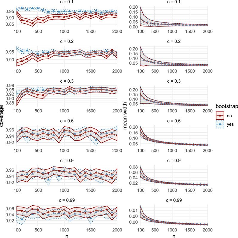
FIGURE 1. Comparisons of coverage (left column) and mean width (right column), between the bootstrap CIs (dashed lines with triangular markers) and the asymptotic CIs (solid lines with circular markers) in MC Study A. Rows represent correlations c, increasing from 0.1 on the top row to 0.99 on the bottom row. The horizontal axes display the sample sizes $n=\mathrm{100,200},\dots ,2000$.

4.2. MC Study B

Here, we choose $\mathcal{D}=t_{\nu }\left(0,\mathbf{\Sigma }\right)$ where $t_{\nu }\left(\mathit{\mu },\mathbf{\Sigma }\right)$ is the multivariate Student t distribution with $\nu \in \left(0,\infty \right)$ degrees of freedom, mean vector $\mathit{\mu }$ and scale matrix $\mathbf{\Sigma }.$ Specifically, the ith sample ${\mathcal{Ƶ}}_n^{\left(i\right)}$, for $i\in \left[N\right]$, we set $\nu =100$ degrees of freedom, and set $\mathbf{\Sigma }$ as the $\left(d+1\right)\times \left(d+1\right)$ covariance matrix in Eq. 13.

For all sample sizes n and correlations c, coverage and width performances are similar to MC Study A (see Supplementary Figures S13 and S14). Of particular interest, in both MC Studies A and B (but not in MC Study C), we observe that for $c=0$, the estimated coverage probability of the asymptotic CI is almost equal to 1, for all sample sizes greater than 10, while the corresponding bootstrap CIs have estimated coverage equal to 0 (Figure 2 left). Despite this, the average CI widths, though large under small samples, are somewhat smaller than those for bootstrap (Figure 2 right).

FIGURE 2

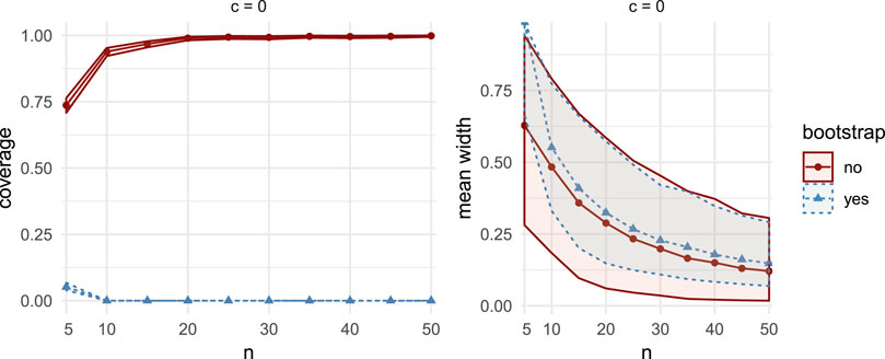
FIGURE 2. Comparisons of coverage (left column) and mean width (right column) between bootstrap CIs (dashed lines with triangular markers) and the asymptotic CIs (solid lines with circular markers) in MC Study B, for correlation $c=0$. The horizontal axes display the sample sizes $n=\mathrm{5,10},\dots ,50$.

4.3. MC Study C

Here, we set ${\mathcal{D}}_i=N_{d+1}\left(0,{\mathbf{\Sigma }}_i\right)$, so that the sample ${\mathcal{Ƶ}}_n^{\left(i\right)}$, for $i\in N$, is drawn from a multivariate normal distribution, with covariance matrix ${\mathbf{\Sigma }}_i$ realized from a Wishart distribution $W_{d+1}\left(\mathbf{\Sigma },\nu \right)$ with scale matrix $\mathbf{\Sigma }$ and ν degrees of freedom. This set up is different from Studies A and B in that the distributions ${\mathcal{D}}_i$, and therefore the population Shapley values $v_1^{\left(i\right)}$, are allowed to differ between samples.

The distribution $W_{d+1}\left(\mathbf{\Sigma },\nu \right)$ can be understood as the distribution of the sample covariance matrix of a sample of size $\nu +1$ from the distribution $N_{d+1}\left(0,\mathbf{\Sigma }\right)$ (cf. Ref. 28). This implies that each covariance matrix ${\mathbf{\Sigma }}_i$ can have non-uniform and negative off-diagonal elements, with variability between the off-diagonal elements increasing as ν decreases. For this study, we set $\nu =100$.

Aside for the case $c=0$, coverage and width statistics are again similar to MC Studies A and B, for all n and c (see Supplementary Material). Interestingly, in all three Studies, for small sample sizes ($n\le 50$), coverage is often higher than for the bootstrap CI, with slightly smaller average widths, as seen in Figure 3 (and in Supplementary Figures S12, S13). For the $c=0$ case, the observed behavior differs from MC Studies A and B, with bootstrap performing comparatively well for large sample sizes (Figures 4, 5).

FIGURE 3

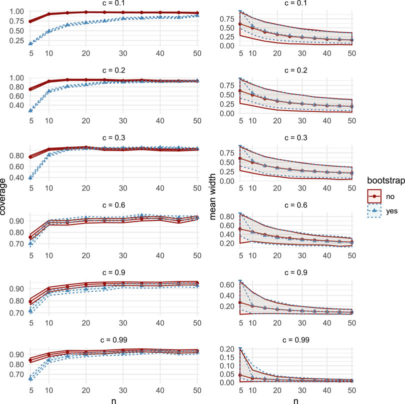
FIGURE 3. Comparisons of coverage (left column) and mean width (right column), between the bootstrap CIs (dashed lines with triangular markers) and the asymptotic CIs (solid lines with circular markers) in MC Study C. Rows represent correlations c, increasing from 0.1 on the top row to 0.99 on the bottom row. The horizontal axes display the sample sizes $n=\mathrm{5,10},\dots ,50$.

FIGURE 4

FIGURE 4. Comparisons of coverage (left column) and mean width (right column) between bootstrap CIs (dashed lines with triangular markers) and the asymptotic CIs (solid lines with circular markers) in MC Study C, for correlation $c=0$. The horizontal axes display the sample sizes $n=\mathrm{5,10},\dots ,50$.

FIGURE 5

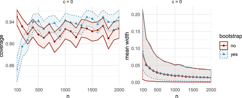
FIGURE 5. Comparisons of coverage (left column) and mean width (right column) between bootstrap CIs (dashed lines with triangular markers) and the asymptotic CIs (solid lines with circular markers) in MC Study C, for correlation $c=0$. The horizontal axes display the sample sizes $n=\mathrm{100,200},\dots ,2000$.

4.4. Computational Benchmarks

From Figure 6, we see that the memory usage (left) and mean execution time (right) for the bootstrap CIs are both higher than that for the asymptotic CIs, and that the ratio increases with sample size given the benchmarking parameters in Table 1. As n increases, asymptotic CIs become increasingly efficient, compared to the bootstrap CIs. On the other hand, as d increases, with n fixed, we expect an increase in the relative efficiency of the bootstrap, since the complexity of calculating $\text{acov}\left({\xi }_j,{\xi }_k\right)$ in Eq. 1 grows faster in d than the complexity of the bootstrap procedure.

FIGURE 6

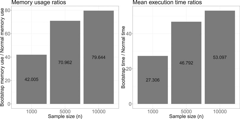
FIGURE 6. Computational benchmark metric ratios of confidence interval estimation using the naïve bootstrap over the asymptotic normality approach.

TABLE 1

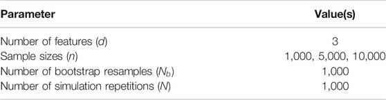
TABLE 1. Parameters for computational benchmarking.

FIGURE 12

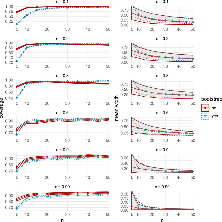
FIGURE 12. Comparisons of coverage (left column) and mean width (right column), between the bootstrap CIs (dashed lines with triangular markers) and the asymptotic CIs (solid lines with circular markers) in MC Study A. Rows represent correlations c, increasing from 0:1 on the top row to 0:99 on the bottom row. The horizontal axes display the sample sizes n = 5;10;50.

FIGURE 13

FIGURE 13. Comparisons of coverage (left column) and mean width (right column), between the bootstrap CIs (dashed lines with triangular markers) and the asymptotic CIs (solid lines with circular markers) in MC Study B. Rows represent correlations c, increasing from 0:1 on the top row to 0:99 on the bottom row. The horizontal axes display the sample sizes n = 5; 10;50.

FIGURE 14

FIGURE 14. Comparisons of coverage (left column) and mean width (right column), between the bootstrap CIs (dashed lines with triangular markers) and the asymptotic CIs (solid lines with circular markers) in MC Study B. Rows represent correlations c, increasing from 0:1 on the top row to 0:99 on the bottom row. The horizontal axes display the sample sizes n = 100; 200;2000.41

FIGURE 15

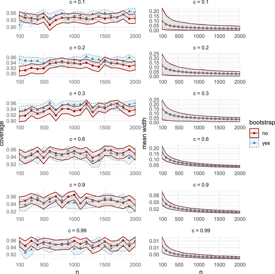
FIGURE 15. Comparisons of coverage (left column) and mean width (right column), between the bootstrap CIs (dashed lines with triangular markers) and the asymptotic CIs (solid lines with circular markers) in MC Study C. Rows represent correlations c, increasing from 0:1 on the top row to 0:99 on the bottom row. The horizontal axes display the sample sizes n = 100; 200; 2000.

4.5. Summary of Results and Recommendations for Use

The most relevant observation is that the widths all appear to shrink at a rate that is comparable to the expected $\sqrt{n}$ convergence dictated by asymptotic normality. The remaining observations below are focused on computational time, sample size, and correlation, in comparison with bootstrap intervals. Below follows a summary of the general tendencies and observations from our results, and recommendations regarding when to use the asymptotic CIs.

• For all correlations c in all three Studies, the estimated coverage probability of asymptotic intervals is above 0.85 for all sample sizes $n\ge 10$.

• For smaller correlations and sample sizes, in particular $c\ge 0.2$ and $n>15$, the lower bound of the confidence interval for coverage never drops below 0.85.

• For all correlations $c\ge 0.3$ and sample sizes $n>100$, the lower bound of the confidence interval for coverage never drops below 0.9.

• For small correlations, in particular $c\le 0.1$ and sample sizes $10\le n\le 100$, the lower bound of the confidence interval for the coverage of the asymptotic CIs never drops below 0.91.

• For $c=0$ and $n\ge 15$, the lower bound of the asymptotic CI for coverage never drops below 0.95 in Studies A and B, while in Study C the lower bound is at least 0.88.

• For sample sizes $15\le n\le 50$, the coverage of the asymptotic CI tends to be higher when c is closer to the boundaries of $\left[\mathrm{0,1}\right]$, as shown in Figure 7.

• The average asymptotic CI width is lower when c is nearer to the boundaries of $\left[\mathrm{0,1}\right]$, see Figure 8.

FIGURE 7

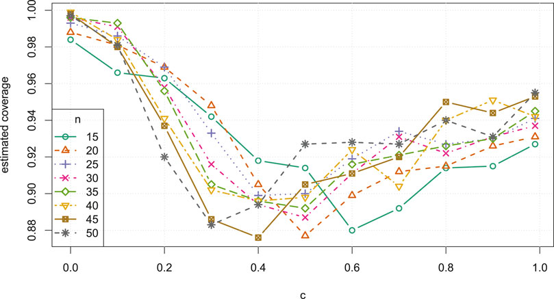
FIGURE 7. Estimated coverage probability versus correlation c, for small samples sizes $n=\mathrm{15,20},\dots ,50$, in MC Study A. The same patterns can be observed for Studies B and C.

FIGURE 8

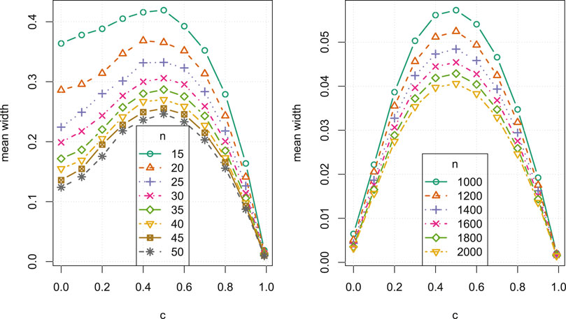
FIGURE 8. Average confidence interval width versus correlation c, for small sample sizes $n=\mathrm{15,20},\dots ,50$ (left) and large sample sizes $n=\mathrm{1000,1200},\dots ,2000$ (right), in MC Study A. The same patterns are present in MC Study B and C.

We now make some general observations which apply to all three Studies. As sample size increases, the estimated coverage initially increases rapidly, as can be seen, for example, in the left column of Figure 3. For small sample sizes between $n=5$ and $n=50$, the asymptotic CIs typically outperform bootstrap CIs, especially when c lies farther from 0.5; there is a clear drop in coverage as c approaches 0.5, for small samples, as can be seen in Figure 7. In many cases, the estimated coverage is above 0.9 for $n\ge 10$. However, empirical coverage does not appear to be an increasing function of sample size in general. On the top row in the left column of Figure 1, we observe one example of a clear and extended dip in coverage for n in $\left[\mathrm{100,1000}\right]$. This gives rise to the general observation that the asymptotic intervals have preferable coverage statistics over bootstrap for small samples, but not for a certain range of large samples, depending on c.

We further observe that, for all n, there is a general increase in the average CI width as c approaches 0.5 from either direction, as in Figure 8. In all Studies, over all sample sizes and correlations, the bootstrap CI average widths were smaller than the asymptotic CI widths by at most 0.0289, and vice versa by at most 0.0667. In general, the asymptotic intervals display favourable widths, though less so near $c=0.5$.

4.6. Recommendations for Use

Based on these observations, we recommend using asymptotic CIs over bootstrap CIs under the following conditions:

(i) Computational time is relevant (e.g., estimating a large number of Shapley values).

(ii) The sample size is small (e.g., $n\le 50$).

(iii) The correlation between explanatory variables and the response variable is expected to be beyond $\pm 0.2$ from 0.5, or when this is where the highest precision is desired.

We note that our observations are made from an incomplete albeit comprehensive set of simulation scenarios. There are of course an infinite number of combinations of simulation cases and thus we cannot guarantee that our observation applies to all possible DGPs.

5. Application: Real Estate and COVID-19

For an interesting application of our methods, in this section we identify significant changes in the behavior of the local real estate market in Melbourne, Australia, between the period 1 February 2019 to 1 April 2019 and the period 1 February 2020 to 1 April 2020. In 2020, this corresponds to an early period of growing public concern regarding the novel coronavirus COVID-19. We obtain the Shapley decomposition of the coefficient of multiple correlation $R^2$ between observed house prices and a number of property features. We also find significant differences in behavior between real estate near and far from the Central Business District (CBD), where near is defined to be within $25\text{km}$ of Melbourne CBD, and far is defined as non-near (see Figure 9). Note that the nature of this investigation is exploratory and expository; our conclusions are not intended to be taken as evidence for the purposes of policy or decision making.

FIGURE 9

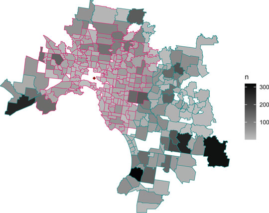
FIGURE 9. Map of Melbourne suburbs included in this study, with greyscale shading to represent sample sizes. Pink dashed polygon borders contain suburbs classified as near to the Central Business District (i.e., $\le 25\text{km}$), and blue solid polygon borders represent those classified as far ($>25\text{km}$). The solid red diamond represents the location of the CBD.

On 1 February the Australian government announced a temporary ban on foreign arrivals from mainland China, and by 1 April a number of social distancing measures were in place. We scraped real estate data from the AUHousePrices website (https://www.auhouseprices.com/), to obtain a data set of $\mathrm{13,291}$ (clean) house sales between 1 January and 18 July in each of 2019 and 2020. We then reduced this date range to capture only the spike in sales observed between 1 February and 1 April (see Figure 10), giving a remaining sample size of 5,110, which was partitioned into the four subgroups in Table 2. By capturing this spike in sales, we hope to detect a significant change in the Shapley values between the same period in 2019 and 2020. Within each of the four subgroups we perform a Yeo-Johnson transformation [29] to reduce any violation of the assumption of joint pseudo-ellipticity.

FIGURE 10

FIGURE 10. Bar plot of sales per day between 1 January and 18 July in 2019 and 2020. Vertical dashed red lines indicate 1 February and 1 April, between which a spike in sales is observed.

TABLE 2

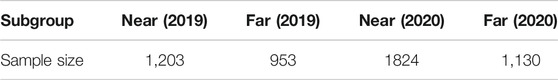
TABLE 2. The four subgroups and their sample sizes after partitioning by distance (where near$:=$ within $25\text{km}$ of CBD), and year of sale in the period 1 February to 1 April 2019 and 2020.

We decompose $R^2$ among the covariates: distance to CBD (CBD); images used in advertisement (images); property land size (land); distance to nearest school (school); distance to nearest station (station); and number of bedrooms $+$ bathrooms $+$ car ports (room); along with the response variable, house sale price (price). We expect the room covariate to act as a proxy for house size. Thus we decompose $R^2$ for the linear model,

$\left(\text{price}\right)={\beta }_0+\mathit{\beta }{\left(\text{CBD},\text{images},\text{land},\text{school},\text{station},\text{room}\right)}^T,{\beta }_0\in \mathrm{ℝ},\mathit{\beta }\in {\mathrm{ℝ}}^{\text{6}}.(14)$

Fitted to each of the four subgroups, we obtain $R^2=0.37$ for model Eq. 14, for each subgroup except for the near (2020) subgroup, for which $R^2=0.39$. The resulting Shapley values and 95% confidence intervals are listed in Table 3, and shown graphically in Figure 11. Also in Figure 11, the corresponding bootstrap CIs are given for completeness, and are almost identical to the asymptotic CIs. From these results we make the following observations regarding attributions of the total variability in house prices explained by model Eq. 14:

(i) In both 2019 and 2020, the attribution for distance to CBD was significantly higher for house sales near to the CBD, compared to house sales farther from the CBD. Correspondingly, the attribution for roominess was significantly lower for house sales near to the CBD.

(ii) Among sales that were near to the CBD, distances to the CBD received significantly greater attribution than both land size and roominess in 2019. Unlike the case for sales that were far from the CBD, these differences remained significant in 2020.

(iii) Distances to stations and schools, as well as images used in advertising, have apparently had little overall impact. In all four subgroups, the attribution for distance to the nearest school is not significantly different from 0. However, distance to a station does receive significantly more attribution among houses that are near to the CBD, compared to those farther away.

(iv) Interestingly, while not a significant result, the number of images used in advertising did appear to receive greater attribution among house sales that were far from the CBD, compared to those near to it.

(v) Among sales that were far from the CBD, land size and roominess both received significantly more attribution than distance to the CBD, in 2019. However, this difference vanished in 2020, with distances to the CBD apparently gaining more attribution, while roominess and land size apparently lost some attribution, in a relative leveling out of these three covariates.

TABLE 3

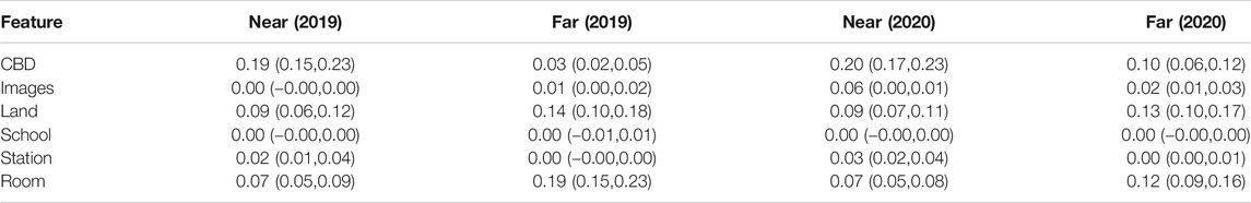
TABLE 3. Shapley values and asymptotic CIs for the covariates of the real estate data.

FIGURE 11

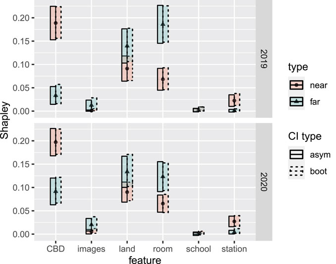
FIGURE 11. Shapley values and associated asymptotic 95% confidence intervals (labelled as CI type “asym”) for each of the six covariates, within the four real estate data subgroups (near/far and 2019/2020). Blue bands and triangle markers represent the near subgroup (i.e., $\le 25\text{km}$ from Central Business District) and red bands with circular markers represent the far subgroup $\left(>25\text{km}\right)$. Beside the asymptotic CIs, the corresponding bootstrap CIs are shown with dashed lines (labeled as CI type “boot”).

Item (i) is perhaps unsurprizing: distances were less relevant far from the city, where price variability was influenced more by roominess and land size. Indeed, we can assume we are less likely to find small and expensive houses far from the CBD. However, the authors find Item (v) interesting: near the city, the behavior did not change significantly during the 2020 period. However, far from the city, the behavior did change significantly, moving toward the near-city behavior. Distance to the city became more important for explaining variability in price, while land size and roominess both became less important, compared with their 2019 estimates. Our initial guess at an explanation was that near-city buyers, with near-city preferences, were temporarily motivated by urgency to buy farther out. However, according to Table 2, the observed ratio of near-city buyers to non-near buyers actually increased in this period, from 1.26 in 2019 to 1.61 in 2020. We will not take this expository analysis further here, but we hope that the interested reader is motivated to take it further, and to this end we have made the data, as well as R and Julia scripts, available at https://github.com/ex2o/shapley_confidence.

6. Discussion

In this work, we focus on regression Shapley values as a means for attributing goodness of fit. There has also been much recent interest in the machine learning literature in using Shapley values to attribute predictions. These approaches, such as SHAP [30], TreeExplainer [31], and Quantitative Input Influence [32] are focused on providing local explanations that depend on the behavior of a fitted model. For more on the differences between prediction, estimation and attribution, see the recent exposition of Ref. 33.

Research into the attribution of goodness of fit using the Shapley value, predates research into attributing predictions. As described in Section 2, regression Shapley values were first introduced in Ref. 10. Then, Ref. 1 advocated for decompositions among exogenously grouped sets of explanatory variables using the both the Shapley and Owen values, where the Owen values are a generalization that permits group attributions.

Our work is the first to determine the asymptotic distribution of the regression Shapley values. In Section 3, we show that under an elliptical (or pseudo-elliptical) joint distribution assumption, the Shapley value decomposition of $R^2\left({\mathcal{Ƶ}}_n\right)$ is asymptotically normal. This involved correcting a number of errors that appeared in the expositions of Lemmas 2 and 3 in prior sources, and stating those results in a notation conforming to the language of cooperative games and set-valued functions. Our result regarding the asymptotic distribution leads immediately to Shapley value confidence intervals and hypothesis tests.

In Section 4, we use Monte Carlo simulations to examine the coverage and width statistics of these asymptotic CIs. We compare the coverage and width statistics for different data generating processes, correlations and sample sizes. In Section 4.5 we provide recommendations for when asymptotic CIs should be used rather than bootstrap CIs. We find that the asymptotic CIs have estimated coverage probabilities of at least 0.85 across all studies, are preferable over the bootstrap CIs for small sample sizes ($n\le 50$), and are often (although not always) favourable for large sample sizes. We discuss the generality of our findings that asymptotic CIs are computationally much more efficient than bootstrap CIs.

In Section 5, we derive asymptotic CIs to Melbourne house prices during a period of altered consumer behavior in the initial stages of the arrival of COVID-19 in Australia. Using the CIs, we identify significant changes in model behavior between 2019 and 2020, and attribute these changes among features, highlighting an interesting direction of future research into the period. Implementations of our methods as well as data sets are openly available for use at https://github.com/ex2o/shapley_confidence.

We aim to use our developments to derive the asymptotic distributions of variance inflation factors and their generalizations [34], as well as the closely related Owen values decomposition of the coefficient of determination for exogenously grouped sets of features [1]. We will also investigate calculating Shapley values capable of uncovering non-linear dependencies and their confidence intervals in future work.

Author’s Note

This manuscript has been released as a pre-print on arXiv [35].

Data Availability Statement

The raw data supporting the conclusions of this article will be made available by the authors, without undue reservation.

Author Contributions

DF Provided Monte Carlo simulations, theoretical contributions, real estate data scraping and analysis, figures, computational benchmarks and general writing. IS Provided real estate data analysis, theoretical contributions, general writing and proofreading. HN Provided theoretical proofs, theoretical contributions, general writing and proofreading.

Conflict of Interest

The authors declare that the research was conducted in the absence of any commercial or financial relationships that could be construed as a potential conflict of interest.

Supplementary Material

The Supplementary Material for this article can be found online at: https://www.frontiersin.org/articles/10.3389/fams.2020.587199/full#supplementary-material

References

1. Huettner, F, and Sunder, M. Decomposing axiomatic arguments for decomposing goodness of fit according to Shapley and Owen values. Electron J Statist. (2012). 6:1239–50. doi:10.1214/12-ejs710

CrossRef Full Text | Google Scholar

2. Efron, B. Computer-intensive methods in statistical regression. SIAM Rev. (1988). 30:421–49. doi:10.1137/1030093

PubMed Abstract | CrossRef Full Text | Google Scholar

3. Baglivo, JA. Mathematica laboratories for mathematical statistics: emphasizing simulation and computer intensive methods. Philadelphia, PA: SIAM (2005).

Google Scholar

4. Steiger, JH, and Browne, MW. The comparison of interdependent correlations between optimal linear composites. Psychometrika (1984). 49:11–24. doi:10.1007/bf02294202

CrossRef Full Text | Google Scholar

5. Hedges, LV, and Olkin, I. Joint distributions of some indices based on correlation coefficients. In: S, Karlin, T, Amemiya, and LA, Goodman, editors Studies in econometrics, time series, and multivariate analysis. Cambridge, UK: Academic Press (1983).

PubMed Abstract | Google Scholar

6. Olkin, I, and Finn, JD. Correlations redux. Psychol Bull (1995). 118:155–64. doi:10.1037/0033-2909.118.1.155

PubMed Abstract | CrossRef Full Text | Google Scholar

7. Seber, GAF, and Lee, AJ. Linear regression analysis. Hoboken, NJ: Wiley (2003).

PubMed Abstract | Google Scholar

8. Greene, WH. Econometric analysis. Upper Saddle River, NJ: Prentice-Hall. (2007).

PubMed Abstract | Google Scholar

9. Cowden, DJ. The multiple-partial correlation coefficient. J Am Stat Assoc. (1952). 47:442–56. doi:10.1080/01621459.1952.10501183

PubMed Abstract | CrossRef Full Text | Google Scholar

10. Lipovetsky, S, and Conklin, M. Analysis of regression in game theory approach. IED Stoch Models Bus Ind Appl. 17, 319–30. doi:10.1002/asmb.446

CrossRef Full Text | Google Scholar

11. Israeli, O (2007). A Shapley-based decomposition of the R-square of a linear regression. J Econ Inequal. 5, 199–212.

Google Scholar

12. Shapley, LS. A value for n-person games. In: HW, Kuhn, and AW, Tucker, editors Contributions to the theory of games. Princeton, NJ: Princeton University Press (1953).

PubMed Abstract | Google Scholar

13. Gromping, U. Relative importance for linear regression R: the package relaimpo. J Stat Softw. (2006). 17, 1–27.

PubMed Abstract | Google Scholar

14. Grömping, U. Estimators of relative importance in linear regression based on variance decomposition. Am Stat. (2007). 61, 139–47. doi:10.1198/000313007x188252

CrossRef Full Text | Google Scholar

15. Young, HP. Monotonic solutions of cooperative games. Int J Game Theory (1985). 14:65–72. doi:10.1007/bf01769885

CrossRef Full Text | Google Scholar

16. Feltkamp, V. Alternative axiomatic characterizations of the shapley and banzhaf values. Int J Game Theory (1995). 24(2):179–86. doi:10.1007/bf01240041

CrossRef Full Text | Google Scholar

17. Kruskal, W. Relative importance by averaging over orderings. Am Am Stat. (1987). 41, 6–10. doi:10.2307/2684310

PubMed Abstract | CrossRef Full Text | Google Scholar

18. Genizi, A. Decomposition of R² in multiple regression with correlated regressors. Stat Sin. (1993). 13:407–20.

PubMed Abstract | Google Scholar

19. Mardia, KV (1970). Measures of multivariate skewness and kurtosis with applications. Biometrika 57:519–30. doi:10.1093/biomet/57.3.519

PubMed Abstract | CrossRef Full Text | Google Scholar

20. Fang, KT, Kotz, S, and Ng, KW. Symmetric multivariate and related distributions. London, UK: Chapman & Hall (1990).

PubMed Abstract | Google Scholar

21. Yuan, K-H, and Bentler, PM. On normal theory and associated test statistics in covariance structure analysis under two classes of nonnormal distributions. Stat Sin. (1999). 9:831–53.

Google Scholar

22. Yuan, K-H, and Bentler, PM. Inferences on correlation coefficients in some classes of nonnormal distributions. J Multivar Anal. (2000). 72:230–48. doi:10.1006/jmva.1999.1858

CrossRef Full Text | Google Scholar

23. Hedges, LV, and Olkin, I. Joint distribution of some indices based on correlation coefficients (1983). Technical Report MCS 81-04262, Stanford University.

PubMed Abstract | Google Scholar

24. van der Vaart, A. Asymptotic statistics. Cambridge, UK: Cambridge University Press (1998).

PubMed Abstract | Google Scholar

25. Seber, GAF. A matrix Handbook for statisticians. New York, NY: Wiley (2008).

Google Scholar

26. Hart, S, and Mas-Colell, A. The potential of the shapley value. Shapley Value (1988). 14:127–37.

PubMed Abstract | Google Scholar

27. Clopper, CJ, and Pearson, ES. The use of confidence or fiducial limits illustrated in the case of the binomial. Biometrika (1934). 26(4):404–13. doi:10.1093/biomet/26.4.404

PubMed Abstract | CrossRef Full Text | Google Scholar

28. Fujikoshi, Y, Ulyanov, VV, and Shimizu, R. Multivariate statistics: high-dimensional and large-sample approximations. Vol. 760. Hoboken, NJ: John Wiley & Sons (2011).

Google Scholar

29. Yeo, I-K, and Johnson, RA. A new family of power transformations to improve normality or symmetry. Biometrika (2000). 87(4), 954–59. doi:10.1093/biomet/87.4.954

PubMed Abstract | CrossRef Full Text | Google Scholar

30. Lundberg, SM, and Lee, S-I. A unified approach to interpreting model predictions. In: I, Guyon, UV, Luxburg, S, Bengio, H, Wallach, R, Fergus, and S, Vishwanathan, editors Advances in neural information processing systems. Vol. 30, London, UK: Curran Associates, Inc (2017). p. 4765–74.

PubMed Abstract | Google Scholar

31. Lundberg, SM, Erion, G, Chen, H, DeGrave, A, Prutkin, JM, Nair, B, et al. From local explanations to global understanding with explainable ai for trees. Nat Mach Intell. (2020). 2(1):56–67. doi:10.1038/s42256-019-0138-9

PubMed Abstract | CrossRef Full Text | Google Scholar

32. Datta, A, Sen, S, and Zick, Y. Algorithmic transparency via quantitative input influence: theory and experiments with learning systems. In: 2016 IEEE symposium on security and privacy (SP); 22–26 May 2016; San Jose, CA. IEEE. (2016). p. 598–617.

Google Scholar

33. Efron, B. Prediction, estimation, and attribution. J Am Stat Assoc. (2020). 115(530):636–55. doi:10.1080/01621459.2020.1762613

PubMed Abstract | CrossRef Full Text | Google Scholar

34. Fox, J, and Monette, G. Generalized collinearity diagnostics. J Am Stat Assoc. (1992). 87(417):178–83. doi:10.1080/01621459.1992.10475190

PubMed Abstract | CrossRef Full Text | Google Scholar

35. Fryer, D, Strumke, I, and Nguyen, H. Shapley value confidence intervals for variable selection in regression models. arXiv preprint arXiv:2001.09593 (2020).

Google Scholar