 Maxime Conjard*†
 Henning Omre†
- Department of Mathematical Sciences, Norwegian University of Science and Technology, Trondheim, Norway
Data assimilation in models representing spatio-temporal phenomena poses a challenge, particularly if the spatial histogram of the variable appears with multiple modes. The traditional Kalman model is based on a Gaussian initial distribution and Gauss-linear forward and observation models. This model is contained in the class of Gaussian distribution and is therefore analytically tractable. It is however unsuitable for representing multimodality. We define the selection Kalman model that is based on a selection-Gaussian initial distribution and Gauss-linear forward and observation models. The selection-Gaussian distribution can be seen as a generalization of the Gaussian distribution and may represent multimodality, skewness and peakedness. This selection Kalman model is contained in the class of selection-Gaussian distributions and therefore it is analytically tractable. An efficient recursive algorithm for assessing the selection Kalman model is specified. The synthetic case study of spatio-temporal inversion of an initial state, inspired by pollution monitoring, suggests that the use of the selection Kalman model offers significant improvements compared to the traditional Kalman model when reconstructing discontinuous initial states.
1 Introduction
Data assimilation in models representing spatio-temporal phenomena is challenging. Most statistical spatio-temporal models are based on assumptions of temporal stationarity, possibly with a parametric, seasonal trend model [1]. We consider spatio-temporal phenomena where the dynamic spatial variables evolve according to a set of differential equations. Such phenomena will, in statistics, normally be modeled as hidden Markov models [2]. The celebrated Kalman model [3] is one of the most frequently used hidden Markov models.
In studies of hidden Markov models, it is natural to distinguish between filtering and smoothing [2]. Filtering entails predicting the spatial variable at a given time with observations up to that point in time. Smoothing entails predicting the spatial variable given observations both at previous and later times. Filtering is naturally based on recursive temporal updating while smoothing appears as more complicated since updating must also be made backwards in time. We focus on a particular smoothing challenge, namely to assess the initial state given observations at later times and we denote the task spatio-temporal inversion.
Spatio-temporal inversion is of interest in many applications. In petroleum engineering, initial water saturation is often unknown. Ensemble smoothing techniques [4–6] are commonly used to evaluate this parameter and improve fluid flow prediction. In air pollution monitoring [7], inverse trajectory methods are used to identify potential source contribution. Source mapping of wildfire origin from airborne smoke observations is a spectacular example [8]. Evaluation of groundwater pollution mostly focuses on the future pollution of the pollutant, but as emphasized in [9], the identification of the heterogeneous source may be complicated.
We study a continuous spatial variable, a random field (RF), with temporal behavior governed by a set of differential equations. The spatio-temporal variable is discretized in space and time, and the hidden Markov model is cast in a Bayesian framework. The prior model consists of an initial spatial model and a forward spatio-temporal model, representing the evolution of the spatio-temporal phenomenon. The likelihood model represents the observation acquisition procedure. The corresponding posterior model, fully defined by the prior and likelihood models, represents the spatio-temporal phenomenon given the available observations. The traditional Kalman model constitutes a very particular hidden Markov model [3] with a Gaussian initial model and a linear forward function with Gaussian error term (Gauss-linear) forward model, and a Gauss-linear likelihood model. Since the class of Gaussian models is closed under linear operations, the posterior distribution is also Gaussian in the Kalman model, and the posterior model parameters are analytically tractable. Based on this posterior Gaussian model, both filtering and smoothing can easily be performed. In particular, the spatio-temporal inversion can be obtained by integrating out the spatial variables at all time points except the initial one, which is a simple task in Gaussian models. Most spatio-temporal models used in statistical studies are defined in the traditional Kalman model framework [10, 11]. Moreover, most of these models are based on spatial stationarity and consider filtering. Their focus is primarily on computational efficiency, not on model flexibility.
The fundamental Gauss-linear assumptions of the traditional Kalman model are often not suitable in real studies. The initial spatial variable may appear as non-Gaussian and/or the forward and/or the likelihood functions are non-linear. In the control theory community, linearizations such as the extended Kalman filter [12] or quantile-based representation such as the unscented Kalman filter [13] are recommended in these cases. These approaches are suitable for models with mild deviations from Gauss-linearity. Statisticians will more naturally use various Monte-Carlo based approaches such as the particle filter [2] or the ensemble Kalman Filter (EnKF) [14]. The particle filter is a sequential Monte Carlo algorithm with data assimilation made by reweighting the particles. To avoid singular solutions, resampling is usually required during the assimilation. The need for resampling makes the definition of an efficient corresponding particle smoother difficult. The EnKF is also a sequential Monte Carlo algorithm with data assimilation based on linear updates of each ensemble member. The sequential linear updates cause the ensemble distribution to drift toward Gaussianity. A corresponding ensemble smoother [15] is available but the ensemble drift toward Gaussianity makes it difficult to preserve non-Gaussianity in the posterior distribution. The discrete representation of the spatial variable makes the spatio-temporal model high-dimensional, and according to [16, 17], the EnKF is preferable to the particle filter in high dimensional models. Lastly, brute force Markov chain Monte Carlo (McMC) [18] algorithms may be used for spatio-temporal inversion, but the increasing coupling of the temporal observations makes these algorithms inefficient. Focus in our study is on the spatial initial state of the spatio-temporal phenomenon, and we aim at reproducing clearly non-Gaussian marginal features, such as multi-modality, skewness and peakedness. Several models with such features are presented in the literature.
In [19], a hidden Markov model with a skew-Gaussian initial model is defined, and for Gauss-linear forward and likelihood models, it is demonstrated that the filtering is analytically tractable. The skew-Gaussian model is based on a selection concept, and the current spatio-temporal model will later be defined along these lines.
In [16, 20–24], the initial model in the hidden Markov model is defined to be a Gaussian mixture model representing multimodality. These studies all consider filtering problems and the filter algorithms are based on a combination of clustering/particle filter and Kalman filter/EnKF. The Gaussian mixture model contains a latent categorical mode indicator, which in a spatial setting must have spatial coupling, for example in the form of a Markov RF [25]. Data assimilation in such categorical Markov RFs, either by particle filter or EnKF, appears as very complicated [23, 24], particularly in a smoothing setting.
The spatio-temporal case we consider in the current study has a non-Gaussian spatial initial model, while both the forward and likelihood models are Gauss-linear. We study this special case since it has a particularly elegant analytical solution. Further, we study spatio-temporal inversion, which entails smoothing to assess the initial spatial variable given observations up to current time, as it constitutes a particularly challenging problem. To our knowledge, no reliable methodology exists for solving such a spatio-temporal inverse problem.
In the hidden Markov model considered in this study, the initial spatial model is assigned a selection-Gaussian RF [26], which may capture multi-modality, skewness and/or peakedness in the spatial histogram of the initial spatial variable. Recall that the forward and likelihood models are assumed to be Gauss-linear. Since the class of selection-Gaussian models is closed under linear operations [26] the posterior model will also be selection-Gaussian. The posterior model parameters are then analytically tractable. A general algorithm for assessing this posterior selection-Gaussian model is defined. Based on this posterior model, both smoothing and filtering can be performed. We denote this special hidden Markov model the selection Kalman model. The class of Gaussian models is a central member in the class of selection-Gaussian models [26], hence one may consider the selection Kalman model to be a generalization of the Kalman model. We develop the results presented above and demonstrate the use of the selection Kalman model on a synthetic case study of spatio-temporal inversion. This entails assessing the initial spatial variable in a dynamic model based on a limited set of observations.
The characteristics of the class of selection-Gaussian models are central in the development of the selection Kalman model properties. These characteristics are thoroughly discussed in [26], which is inspired by the results presented in [27, 28]. In these papers, the general concept of the selection-Gaussian pdf is defined in a probabilistic setting. In [19], the one-sided selection concept is used to define a skew Kalman filter in a non-spatial setting.
In this paper
In Section 2, the problem is set. In Section 3, the traditional Kalman model is cast in a Bayesian hidden Markov model framework. The generalization to the selection Kalman model is then defined, and the analytical tractability is investigated. Further a general recursive algorithm for assessing the posterior distribution is specified. In Section 3, a synthetic case study of the advection-diffusion equation is discussed to showcase the ability of the selection Kalman model to solve the spatio-temporal inversion problem. The goal is to reconstruct the initial state. Results from the selection Kalman model and the traditional Kalman model are compared. In section 4, conclusions are presented.
2 Problem Setting
The case is defined in a spatio-temporal setting. Consider the variable
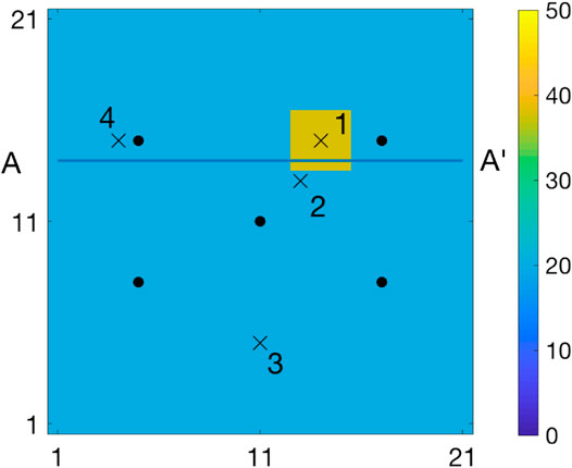
FIGURE 1. Initial state with observation locations
The spatio-temporal variable evolves in time,
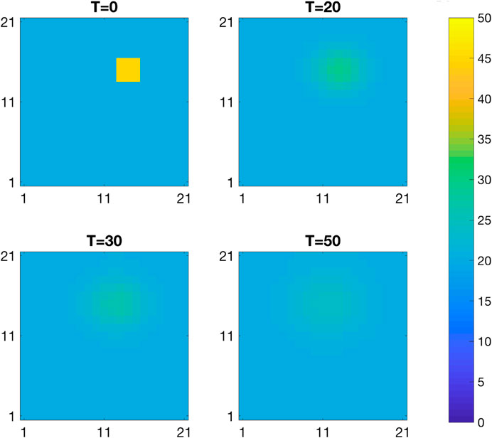
FIGURE 2. Spatio-temporal diffusion.

FIGURE 3. Observations at the observation locations and true curve.
3 Model Definition
Consider the unknown temporal n-vector
3.1 Bayesian Inversion
The Kalman type model, phrased as Bayesian inversion, requires the specification of a prior model for
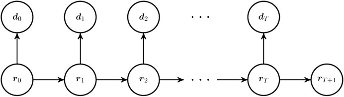
FIGURE 4. Graph of the hidden Markov model.
3.1.1 Prior Model
The prior model on
Initial Distribution
The prior distribution for the initial state
Forward Model
The forward model given the initial state
with,
where
3.1.2 Likelihood Model
The likelihood model on
with,
where
3.1.3 Posterior Model
Bayesian inversion endeavors to assess the posterior distribution of
which is a non-stationary Markov chain for the hidden Markov model with a likelihood model in factored form as defined above [29]. Assessing such a posterior distribution is usually difficult as both the normalizing constant and the conditional transition matrices are challenging to calculate.
3.2 Kalman Type Models
The current study is limited to Kalman type models. They comprise an initial and a process part.
Initial Distribution
The initial distribution is identical to the initial distribution of the prior model
Process Model
The process model includes the forward model and likelihood models defined in Section 3.1. It thus characterizes the process dynamics and the observation acquisition procedure. The forward model is defined by,
with forward
with the observation
3.3 Traditional Kalman Model
The traditional Kalman model is defined by letting the initial distribution be in the class of Gaussian pdfs,
with initial expectation n-vector
This traditional Kalman model is analytically tractable. The posterior distribution
• The initial model
• The conditional model
By recursion, we obtain that
From the joint Gaussian pdf
3.4 Selection Kalman Model
The selection Kalman model is defined by letting the initial distribution be in the class of selection-Gaussian pdfs [27, 28]. This class is defined by considering an auxilary n-vector
with expectation n-vector
with the expectation q-vector
with
with the covariance
This class of pdfs is parametrized by
Four one-dimensional selection-Gaussian pdfs are displayed in Figure 5 in order to demonstrate the influence of the selection set
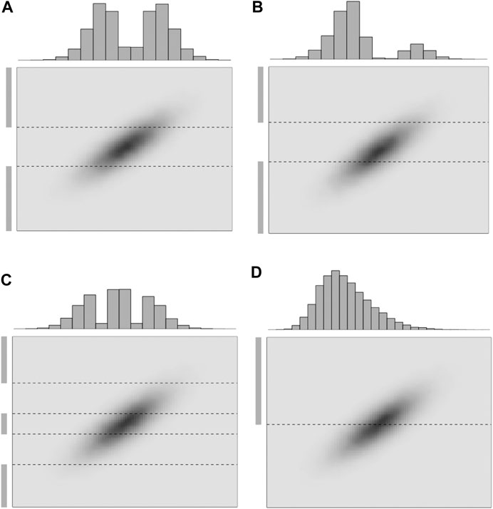
FIGURE 5. Realizations of 1D selection-Gaussian pdfs (histogram) with varying selection sets
Note that assigning a null-matrix to
• The initial model
• The conditional model
By recursion, we obtain that
Consider the augmented
Algorithm 1 provides the Gaussian pdf of the
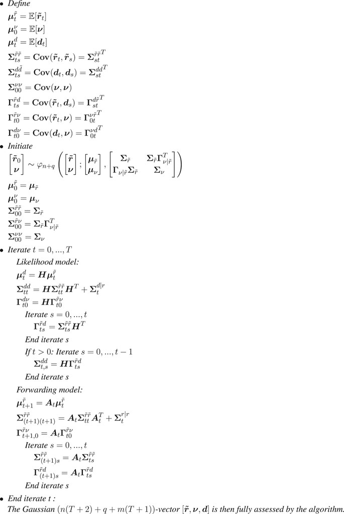
Algorithm 1. Joint Selection Kalman Model
4 Synthetic Study
The synthetic study is introduced in Section 2, and we discuss it in larger detail in this section.
4.1 Model
Consider a discretized spatio-temporal continuous RF representing the evolution of a temperature field
The initial temperature field
with
where the
The observations are acquired at
where the observation
The forward and likelihood models are Gauss-linear. In order to fully defined the selection Kalman model and traditional Kalman model, we must specify the prior distribution for the initial temperature field for both approaches.
We assume we know the initial temperature field has large areas with low temperatures in the range
The prior distribution is set to be selection-Gaussian for the selection Kalman model. Such a prior model can represent multimodality. The model is constructed according to [26] and is defined considering an auxiliary discretized stationary Gaussian RF,
with expectation and variance levels,
with coupling parameter
Define a separable selection set
Note that after selection on the auxiliary variable
The parameters values are listed in Table 1 and they are chosen to reflect what is assumed about the initial temperature field. The prior marginal distribution is bimodal, the dominant mode is centered about
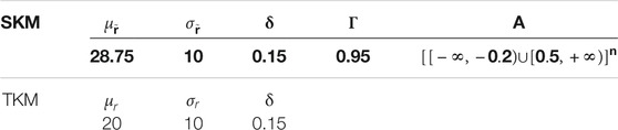
TABLE 1. Parameter values for the selection Gaussian initial model (SKM) and the Gaussian initial model (TKM).

FIGURE 6. Prior marginal distribution of the initial temperature field for the selection Kalman model.
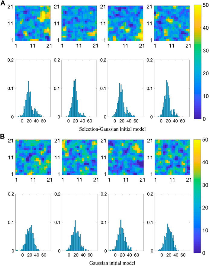
FIGURE 7. Realizations from the prior distribution of the initial state; maps (upper), spatial histograms (lower).
The prior distribution for the traditional Kalman model is Gaussian and is defined as,
with expectation and variance levels,
Figure 7B displays four realizations with associated spatial histograms from the prior distribution for the traditional Kalman model. The mean and variance levels are chosen so that the prior covers the assumed range for the high and low temperature areas as can be seen in the spatial histograms.
Figure 7B can be compared to Figure 7A, and one observes that only the selection-Gaussian distribution can capture bi-modality in the spatial histograms. In studies with real data, the prior model specification must of course be based on experience with the phenomenon under study.
In the next section, we demonstrate the effect of specifying different initial models in the spatio-temporal inversion model.
4.2 Results
The challenge is to restore
1. Marginal pdfs at four monitoring locations represented by crosses and numbered
and similarly for
2. Spatial prediction based on a marginal maximum a posteriori (MMAP) criterion,
and similarly for
3. The MMAP prediction and the associated 0.80 prediction interval along a horizontal profile A-A’, see Figure 1. The prediction interval is computed as the highest density interval (HDI) [31], which entails that the prediction intervals may consist of several intervals for multimodal posterior pdfs.
4. Realizations From the Posterior Pdfs
Figure 8 displays the marginal posterior pdfs based on the selection Kalman model at the four monitoring locations, vertically, for increasing current time T, horizontally. At current time
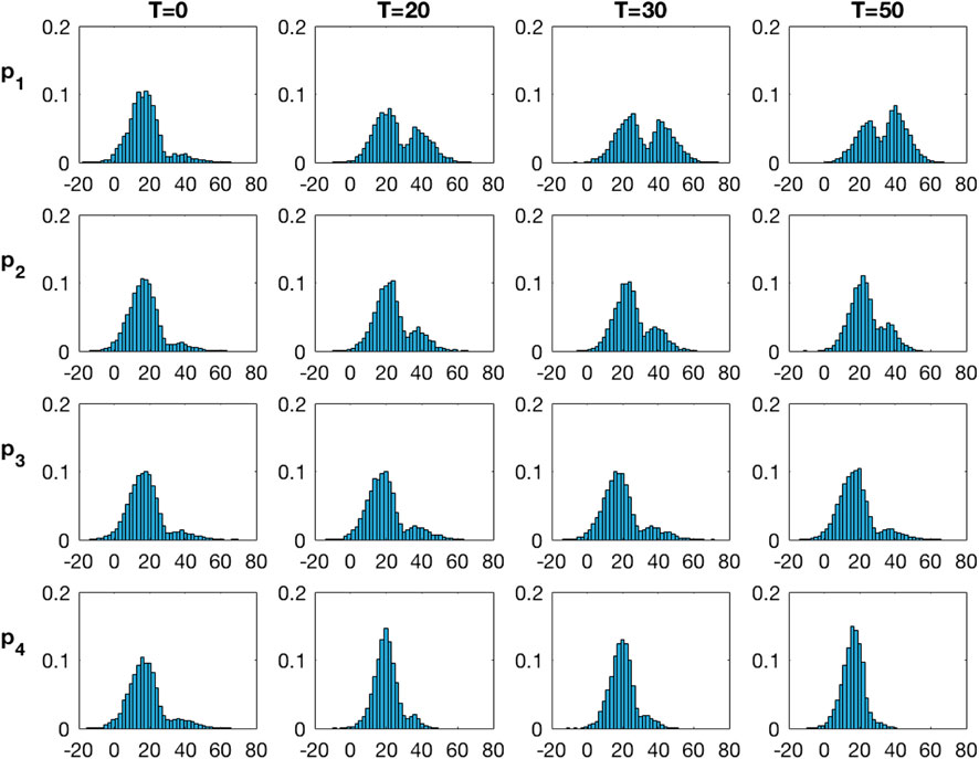
FIGURE 8. Marginal pdfs at monitoring locations for increasing current time T from the inversion with the selection Kalman model.
Figure 9 displays the marginal pdfs from the traditional Kalman model. These marginal posterior pdfs are also virtually identical at current time
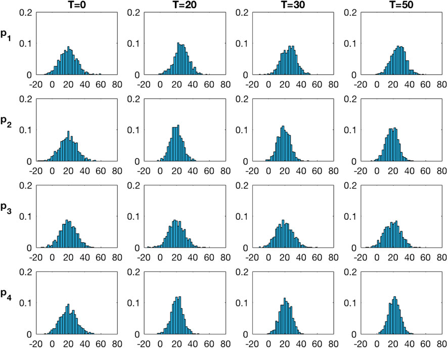
FIGURE 9. Marginal pdfs at monitoring locations for increasing current time T from the inversion with the traditional Kalman model.
The upper panels of Figure 10 display the MMAP spatial prediction based on the selection Kalman model for increasing current time T. At current time
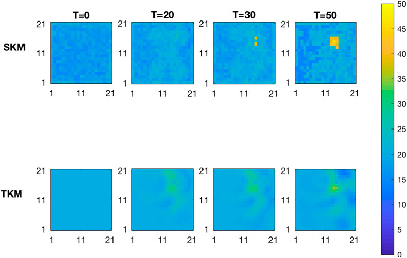
FIGURE 10. MMAP predictions of the initial state for increasing current time T from the inversion with the selection Kalman model (SKM-upper) and with the traditional Kalman model (TKM-lower).
We evaluate the root mean square error (RMSE) values of the two models at time
Figure 11 displays the MMAP predictions with associated 0.80 prediction intervals along the horizontal profile A-A’. The prediction from the selection Kalman model captures the yellow area while the prediction from the traditional Kalman model barely indicates the yellow area. The prediction intervals follow the same pattern. Note, however, that the prediction intervals of the selection Kalman model may appear as two intervals close to the yellow area since the marginal posterior models are bimodal. By using the selection Kalman model, the location, spatial extent and value of the yellow area is very precisely predicted at current time
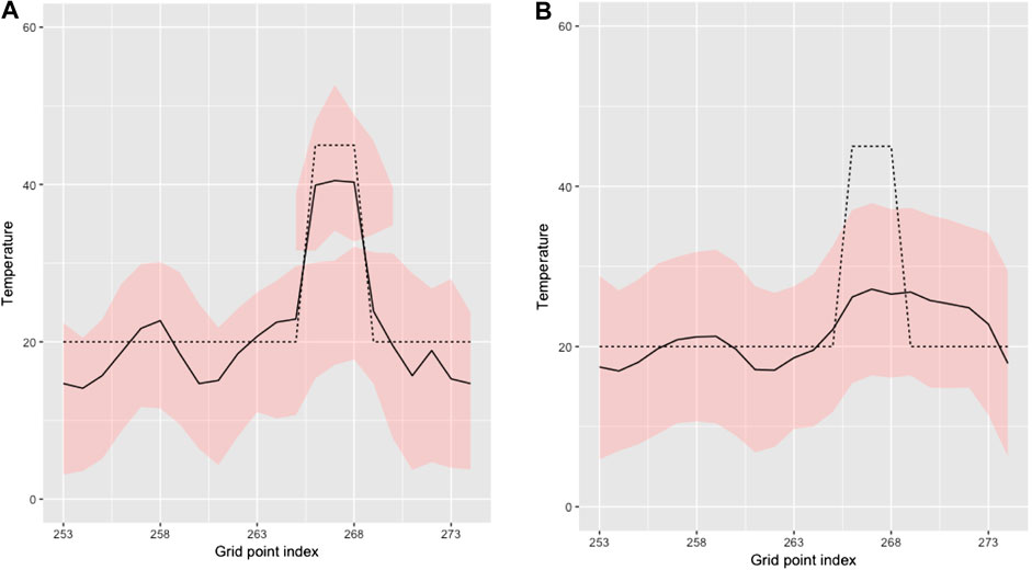
FIGURE 11. MMAP predictions (solid black line) with HDI 0.8 (red) intervals in cross section A-A′ of initial state at current time
Figure 12 displays realizations from the posterior pdfs at
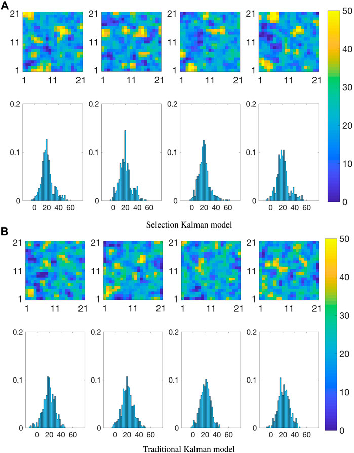
FIGURE 12. Realizations from the posterior distribution of the initial state at current time
Conditioning on the observed data takes the same time for both methods but the selection Kalman model requires sampling from a high dimensional truncated Gaussian pdf in order to evaluate the posterior distribution which means that the computational demand for the selection Kalman model is higher than that of the traditional Kalman model. For
To demonstrate the generality of the selection Kalman model, we define an alternative true initial state with two yellow areas, see Figure 13A. We used the same model parameters as in the primary case. The prior distribution for both the selection Kalman model and the traditional Kalman model are identical to the first case. Note in particular that the number of yellow areas is not specified. The observed time series will of course be different, see Figure 13B. These time series have many similarities with the ones from the primary case. We inspect the marginal pdfs at two monitoring locations, one inside each yellow area, as they evolve with current time T, see Figure 14A. Both marginal pdfs are identical at current time T = 0, and as current time T increases the height of the high-value mode increases, indicating that both monitoring locations are within the yellow areas. In Figure 14B the corresponding MMAP predictions are displayed for increasing current time T. We observe that location, areal extent and value of both yellow areas are well reproduced, but not as well as for the first case since identifying two sources is more complicated. The identification challenge is of course increasing with an increasing number of yellow areas. Figure 14B also displays the MMAP prediction for the traditional Kalman model for the two-yellow-area case, where location, areal extent and value are hard to evaluate, similarly to the first test case.
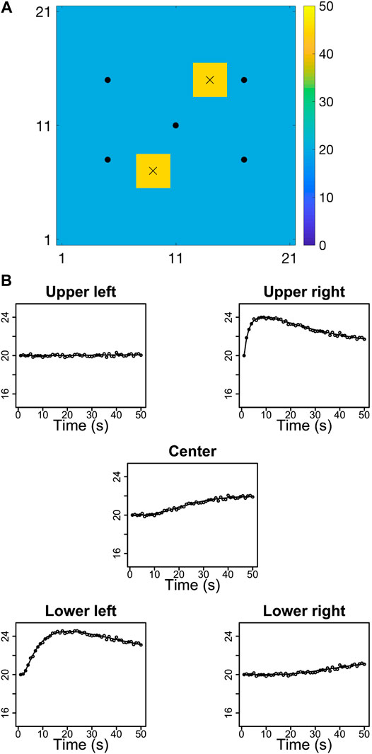
FIGURE 13. Set up from the two yellow area test case.
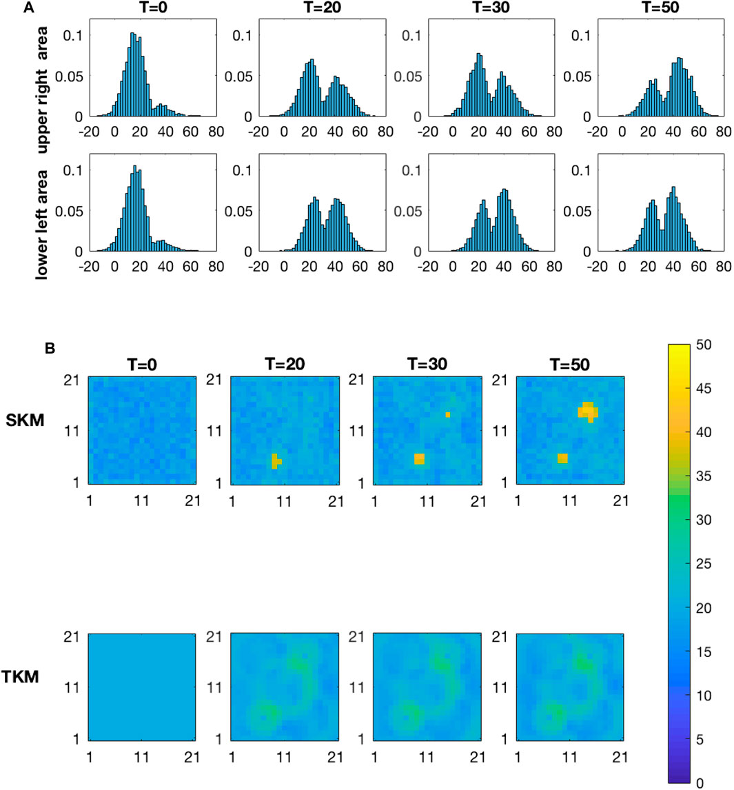
FIGURE 14. Results from the two-yellow-area test case.
5 Conclusion
We define a selection Kalman model based on a selection-Gaussian initial distribution and Gauss-linear dynamic and observation models. This model may represent spatial phenomena with initial states with spatial histograms that are multimodal, skewed and/or peaked. The selection Kalman model is demonstrated to be contained in the class of selection-Gaussian distributions and hence analytically tractable. The analytical tractability makes the assessment of the selection-Gaussian posterior model fast and reliable. Moreover, an efficient recursive algorithm for assessing the selection Kalman model is specified. Note that the traditional Kalman model is a special case of the selection Kalman model, hence the latter can be seen as a generalization of the former.
A synthetic spatio-temporal inversion case study with Gauss-linear forward and observation models is used to demonstrate the characteristics of the methodology. We specify both a selection Kalman model and a traditional Kalman model and evaluate their ability to restore the initial state based on the observed time series. The time series are noisy observations of the variable of interest collected at a set of sites. The selection Kalman model outperforms the traditional Kalman model. The former model identifies location, areal extent and value of the yellow area very reliably. The traditional Kalman model only provides blurry indications with severe under-prediction of the yellow area. We conclude that for spatio-temporal inversion where the initial spatial state has bimodal or multimodal spatial histograms, the selection Kalman model is far more suitable than the traditional Kalman model.
The selection Kalman model has potential applications far beyond the simple case evaluated in this case study. For all spatio-temporal problems where multimodal spatial histograms appear, the selection Kalman model should be considered. The model can easily be extended to a selection extended Kalman model, along the lines of the extended Kalman model. A more challenging and interesting extension is the definition of a selection ensemble Kalman model including non-linear dynamic and observation models. Research along these lines is currently taking place.
Data Availability Statement
The original contributions presented in the study are included in the article/Supplementary Material, further inquiries can be directed to the corresponding author.
Author Contributions
MC and HO contributed equally to this manuscript in every matter except implementation for which was carried out exclusively by MC.
Funding
The research is a part of the Uncertainty in Reservoir Evaluation (URE) activity at the Norwegian University of Science and Technology (NTNU).
Conflict of Interest
The authors declare that the research was conducted in the absence of any commercial or financial relationships that could be construed as a potential conflict of interest.
Acknowledgments
This manuscript is a rewrite of a preprint which can be found at https://arxiv.org/abs/2006.14343.
Supplementary Material
The Supplementary Material for this article can be found online at: https://www.frontiersin.org/articles/10.3389/fams.2021.636524/full#supplementary-material.
References
1. Handcock, MS, and Wallis, JR. An approach to statistical spatial-temporal modeling of meteorological fields. J Am Stat Assoc (1994). 89:368–78. doi:10.1080/01621459.1994.10476754
2. Cappé, O, Moulines, E, and Ryden, T. Inference in hidden Markov models (Springer series in statistics). Berlin, Heidelberg: Springer-Verlag (2005).
3. Kalman, RE. A new approach to linear filtering and prediction problems. J Basic Eng (1960). 82:35–45. doi:10.1115/1.3662552
4. Emerick, AA, and Reynolds, AC. Ensemble smoother with multiple data assimilation. Comput Geosci (2013). 55:3–15. doi:10.1016/j.cageo.2012.03.011
5. Evensen, G, Raanes, PN, Stordal, AS, and Hove, J. Efficient implementation of an iterative ensemble smoother for data assimilation and reservoir history matching. Front Appl Math Stat (2019). 5:47. doi:10.3389/fams.2019.00047
6. Liu, M, and Grana, D. Time-lapse seismic history matching with iterative ensemble smoother and deep convolutional autoencoder. Geophysics (2019). 85:1–63. doi:10.1190/geo2019-0019.1
7. Hopke, PK. Review of receptor modeling methods for source apportionment. J Air Waste Manag Assoc (2016). 66:237–59. doi:10.1080/10962247.2016.1140693
8. Cheng, MD, and Lin, CJ. Receptor modeling for smoke of 1998 biomass burning in Central America. J Geophys Res Atmos (2001). 106:22871–86. doi:10.1029/2001JD900024
9. Kjeldsen, P, Bjerg, PL, Rügge, K, Christensen, TH, and Pedersen, JK. Characterization of an old municipal landfill (Grindsted, Denmark) as a groundwater pollution source: landfill hydrology and leachate migration. Waste Manage Res (1998). 16:14–22. doi:10.1177/0734242X9801600103
10. Wikle, CK, and Cressie, N. A dimension-reduced approach to space-time Kalman filtering. Biometrika (1999). 86:815–29. doi:10.1093/biomet/86.4.815
11. Todescato, M, Carron, A, Carli, R, Pillonetto, G, and Schenato, L. Efficient spatio-temporal Gaussian regression via Kalman filtering. Automatica (2020). 118:109032. doi:10.1016/j.automatica.2020.109032
13. Julier, SJ, and Uhlmann, JK. New extension of the Kalman filter to nonlinear systems. In: I Kadar, editor. Signal processing, sensor fusion, and target recognition VI (SPIE), 3068 (1997). p. 182–93. doi:10.1117/12.280797
14. Evensen, G. Sequential data assimilation with a nonlinear quasi-geostrophic model using Monte Carlo methods to forecast error statistics. J Geophys Res (1994). 99:101–43. doi:10.1029/94JC00572
15. Evensen, G, and van Leeuwen, PJ. An ensemble Kalman smoother for nonlinear dynamics. Monthly Weather Rev (2000). 128:1852–67. doi:10.1175/1520-0493(2000)128<1852:AEKSFN>2.0.CO;2
16. Li, R, Prasad, V, and Huang, B. Gaussian mixture model-based ensemble Kalman filtering for state and parameter estimation for a PMMA process. Processes (2016). 4:9. doi:10.3390/pr4020009
17. Katzfuss, M, Stroud, JR, and Wikle, CK. Ensemble Kalman methods for high-dimensional hierarchical dynamic space-time models. J Am Stat Assoc (2020). 115:866–85. doi:10.1080/01621459.2019.1592753
18. Robert, C, and Casella, G. Monte Carlo statistical methods. Springer Texts in Statistics. New York, NY: Springer (2005).
19. Naveau, P, Genton, MG, and Shen, X. A skewed Kalman filter. J Multivariate Anal (2005). 94:382–400. doi:10.1016/j.jmva.2004.06.002
20. Ackerson, G, and Fu, K. On state estimation in switching environments. IEEE Trans Automatic Control (1970). 15:10–7. doi:10.1109/TAC.1970.1099359
21. Chen, R, and Liu, JS. Mixture Kalman filters. J R Stat Soc Ser B (Statistical Methodology) (2000). 62:493–508. doi:10.1111/1467-9868.00246
22. Smith, KW. Cluster ensemble kalman filter. Tellus A (2007). 59:749–57. doi:10.1111/j.1600-0870.2007.00246.x
23. Dovera, L, and Della Rossa, E. Multimodal ensemble Kalman filtering using Gaussian mixture models. Comput Geosciences (2011). 15:307–23. doi:10.1007/s10596-010-9205-3
24. Bengtsson, T, Snyder, C, and Nychka, D. Toward a nonlinear ensemble filter for high-dimensional systems. J Geophys Res Atmos (2003). 108. doi:10.1029/2002JD002900
25. Ulvmoen, M, and Omre, H. Improved resolution in Bayesian lithology/fluid inversion from prestack seismic data and well observations: Part 1—methodology. Geophysics (2010). 75(2):R21–R35. doi:10.1190/1.3294570
26. Omre, H, and Rimstad, K. Bayesian spatial inversion and conjugate selection Gaussian prior models. Methodology. Preprint: arXiv:1812.01882 (2018).
27. Arellano-Valle, RB, Branco, MD, and Genton, MG. A unified view on skewed distributions arising from selections. Can J Stat (2006). 34:581–601. doi:10.1002/cjs.5550340403
28. Arellano-Valle, R, and del Pino, G. From symmetric to asymmetric distributions: a unified approach. In: M Genton, editor. Skew-elliptical distributions and their applications: a journey beyond normality. New York, NY: Chapman and Hall/CRC) (2004). p. 113–33.
29. Moja, S, Asfaw, Z, and Omre, H. Bayesian inversion in hidden Markov models with varying marginal proportions. Math Geosci (2018). 51:463–84. doi:10.1007/s11004-018-9752-z
30. Robert, CP. Simulation of truncated normal variables. Stat Comput (1995). 121–5. doi:10.1007/BF00143942
Keywords: inverse problem, spatio-temporal variables, Kalman model, multimodality, data assimilation
Citation: Conjard M and Omre H (2021) Spatio-Temporal Inversion Using the Selection Kalman Model. Front. Appl. Math. Stat. 7:636524. doi: 10.3389/fams.2021.636524
Received: 01 December 2020; Accepted: 11 January 2021;
Published: 27 April 2021.
Edited by:
Xiaodong Luo, Norwegian Research Institute, NorwayReviewed by:
Neil Chada, King Abdullah University of Science and Technology, Saudi ArabiaZheqi Shen, Hohai University, China
Copyright © 2021 Conjard and Omre. This is an open-access article distributed under the terms of the Creative Commons Attribution License (CC BY). The use, distribution or reproduction in other forums is permitted, provided the original author(s) and the copyright owner(s) are credited and that the original publication in this journal is cited, in accordance with accepted academic practice. No use, distribution or reproduction is permitted which does not comply with these terms.
*Correspondence: Maxime Conjard, bWF4aW1lLmNvbmphcmRAbnRudS5ubw==
†These authors have contributed equally to this work