 Gayan Dharmarathne
 Anca Hanea
 Andrew P. Robinson
- 1Department of Statistics, University of Colombo, Colombo, Sri Lanka
- 2Centre of Excellence for Biosecurity Risk Analysis, University of Melbourne, Parkville, Vic, Australia
Structured expert judgement (SEJ) is a suite of techniques used to elicit expert predictions, e.g. probability predictions of the occurrence of events, for situations in which data are too expensive or impossible to obtain. The quality of expert predictions can be assessed using Brier scores and calibration questions. In practice, these scores are computed from data that may have a correlation structure due to sharing the effects of the same levels of grouping factors of the experimental design. For example, asking common questions from experts may result in correlated probability predictions due to sharing common question effects. Furthermore, experts commonly fail to answer all the needed questions. Here, we focus on (i) improving the computation of standard error estimates of expert Brier scores by using mixed-effects models that support design-based correlation structures of observations, and (ii) imputation of missing probability predictions in computing expert Brier scores to enhance the comparability of the prediction accuracy of experts. We show that the accuracy of estimating standard errors of expert Brier scores can be improved by incorporating the within-question correlations due to asking common questions. We recommend the use of multiple imputation to correct for missing data in expert elicitation exercises. We also discuss the implications of adopting a formal experimental design approach for SEJ exercises.
1 Introduction
Expert elicitation refers to employing formal procedures for obtaining and combining expert judgments when data are missing, sparse, or of very poor quality, and decisions are imminent. Experts can be asked to predict the outcome and/or likelihood of future events, or to estimate unknown quantities which may be related to the consequences of such events. In both cases experts are often required to express their uncertainty numerically, either through probabilities of event occurrence, or through estimates on a continuous scale that can characterise potential ranges of unknown variables.
Even though expert judgements can be very useful when data are absent, they can be prone to contextual biases that can lead to poor judgements and consequently poor decisions. Structured protocols aim to mitigate these biases and to treat expert data collection as much as possible as any experimental data collection process, that is rigorous, transparent and following scientific principles. By doing so, they aim to increase the accuracy of the resulting judgements when compared to unstructured, informal expert elicitations.
One of the many important steps in a structure expert judgement (SEJ) elicitation protocol is the formulation of questions for experts. Several formats proved to be intuitive and are thought to mitigate biases. In this research we are interested in the elicitation of probabilities of future events (using a SEJ protocol), and their evaluation.
Obtaining the best possible predictions for future events is a relevant topic in any application area, but the latest developments arise from extensive research in the intelligence analysis field. Several massive projects were undertaken recently, for example the Good Judgment project and the Cosmic Bazaar described in the [1].
In order to evaluate/validate elicited probabilities, a validation dataset is necessary. This validation dataset consists of calibration questions, which are questions for which the answers are known, or will become known soon after the elicitation. Using such questions will allow the analysts to check the quality of the expert predictions against the truth. Several measures of quality can be used (e.g., calibration, informativeness, accuracy), but in this research and in the context of eliciting the probability of events occurrences, we focus on the accuracy measure. We define the accuracy of an expert prediction in terms of the Brier score.
1.1 Brier Scores
The Brier score was always one of the most popular measures of performance used to evaluate experts’ probabilistic predictions. It is extensively used in the most recent research on the topic as well, see e.g., [2–4]. In the above mentioned piece from the Economist, someone who trains British intelligence analysts mentions that experts become “obsessed with their Brier scores.” A reason for this obsession may be that constant feedback may improve long term performance, and in turn, this improvement is visible on the Brier scores.
We now detail the mathematical formulation of the score. Assume several experts predict N events. For each expert we can calculate their accuracy per question, or their long term accuracy calculated based on all their N predictions. This long term accuracy can be calculated using the average Brier score. Average Brier scores are typically computed by obtaining average squared deviations between the predicted probabilities of the event occurrence and their outcomes. Eq. 1 provides the originally defined Brier score as an average measure of prediction accuracy over a set of N events, each with n possible outcomes [5].
where
An alternative definition for binary events is given in Eq. 2 [6].
Here,
Even though Brier scores are calculated as single/point values, it is important to acknowledge their variability when calculated from different sets of calibration questions. The scores depend on the number of questions answered, and also on question difficulty, question base rate, and any other source of inherent uncertainty.
To robustly compare expert performance (here, prediction quality), ideally, the same set of questions should be answered by all experts in the comparison. In reality, very often experts only answer a subset of questions that they feel comfortable answering. Moreover, in certain settings, experts are only presented with subsets from a larger set of questions, to distribute the work and decrease the elicitation burden. This practice however renders the comparison of their accuracy scores less reliable. To mitigate this lack of reliability, Brier scores are often presented together with standard errors or confidence intervals [7,8], both calculated based on the (faulty) assumption that the observations are independent.
1.2 Independence of Observations
Experts’ predicted probabilities are not independent, because they answer overlapping sets of questions. This induces a potential dependence/correlation structure between answers which should be taken into account in ongoing analysis. Ignoring this potential dependence is not atypical in the analysis of elicited data; we label this the stand-alone approach.
Even more dependence between answers is introduced in cases when the questions are perceived as easy or hard to more than one expert. In this situation their errors might be correlated to one another. Furthermore, cognitive frailties that are known to introduce bias, such as the halo effect1will likely introduce bias to more than one expert, which increases dependence. The consequence of these correlation structures is that the estimates of the standard errors do not have the intended statistical properties.
To fix ideas, suppose standard errors of expert Brier scores are estimated in an experiment by asking 20 calibration questions to each of 10 experts. The stand-alone approach pretends that there are 200 questions, that is, 20 for each expert, and ignores the potential correlation structure that is induced in the probability predictions by asking all experts the same questions. The assumption of independent errors will be violated if we apply standard statistical methods ignoring potential correlations between observations. It will result in obtaining inaccurate experiment-level standard error estimates of model parameters [9].
Therefore, in this analysis we focus on improving the accuracy of the estimated standard errors of expert Brier scores by incorporating the correlations between probability predictions that are due to the effects of common questions. The above discussed issue of the impact of correlated observations on the accuracy of the standard error estimates has been discussed under the “design effect” of cluster sampling in [10]. According to that the design effect can be large if the units belong to a same group are highly similar as implied by obtaining a higher intra-class correlation coefficient. Furthermore, standard error estimates can be substantially distorted even for a relatively small intra-class correlation.
As a candidate correction to assess the likely magnitude, note that the structure of the experiment as described is analogous to a cluster sample, where the calibration questions are the clusters. [11] discussed a correction procedure for the standard error estimates through the computation of effective sample sizes in two-stage cluster sampling as
where
1.3 Experimental Design
The original definition in Eq. 1 implies that the Brier scores can be computed for events with multiple outcomes if the probabilities of the occurrence of each outcome are predicted. In this study we restrict our attention to binary events (that either occur or not).
Hence, we derive Brier scores similar using Eq. 2. We employ a statistical model based approach to compute expert Brier scores in which the observations of the model are defined by considering both the experts and the questions. Thus,
where
The above model can generally be fitted in situations where the observations of a certain response variable of interest are obtained under different conditions in different treatment groups. The population means of responses are to be estimated in each treatment group and they are estimated by the corresponding sample means within groups. It is not necessary to have an equal number of responses in each treatment group. The treatment groups in our context are the experts and the squared deviations between the predicted probabilities and the outcomes of events are the responses of interest. Obtaining the sample means of responses is equivalent to computing experts’ Brier scores using the Eq. 2. Hence, the above linear model gives mean estimates that are identical to the typical experts’ Brier scores irrespective of whether the experts have predicted all the events or not.
As mentioned above, the typical computation of expert Brier scores fails to capture the potential correlation structure that is induced in the probability predictions by asking common questions. The independence assumption of
1.4 Missing Data
Human judges (even experts) may prefer to assess only the subsets of events of which they feel comfortable to offer coherent predictions in practice [13]. If expert Brier scores are computed using the probability predictions of different subsets of events, then the comparison of the prediction accuracy of experts using Brier scores can be challenging and perhaps may be less meaningful [14,15]. Hence, in order to enhance the comparability of experts’ Brier scores, it is important to compute Brier scores by adjusting for the missing probability predictions of events by experts. From a statistical point of view, ignoring missing values causes to obtain biased estimates of parameters and increase their standard error estimates in general. In addition to that, the statistical power of tests can be decreased and the generalizability of results can be weakened [16].
Missing data are traditionally treated by listwise deletion, a method that simply ignores cases with missing values for any of the variables and analyses the remaining data. This approach is also known as the complete case (or available case) analysis [17]. It is applied in the typical computation of experts Brier scores by ignoring missing predictions. [14,15] have discussed the drawbacks of comparing experts’ Brier scores computed from different sets of questions and suggested that missing data should not be discarded lightly in computing these scores. Adopting a modeling framework, such as mixed-effects model, provides a basis for imputation, which is a statistical correction for missing values. Hence, in this paper, we focus on assessing the effectiveness of employing mixed-effect models to impute missing probability predictions in computing experts’ Brier scores. The description of the selected imputation methods can be found in Section 2.4.
2 Methods
2.1 Motivating Example: The Intelligence Game Data
The Intelligence Advanced Research Projects Activity (IARPA) is an organization within the Office of the Director of National Intelligence in United States of America (United States). IARPA is responsible for leading research to overcome difficult challenges relevant to the United States Intelligence Community. In 2010, IARPA announced a program called the Aggregative Contingent Estimation (ACE) which aimed to “dramatically enhance the accuracy, precision and timelines of forecasts for a broad range of events types, through the development of advanced techniques that elicit, weight and combine the judgements of many intelligence analysts” [7]. The program was designed as a four year forecasting tournament to predict the probabilities of the occurrence of global events on geopolitical, economic, and military sectors. Five collaborative research teams were involved in a competition. This forecasting tournament was called the “Intelligence Game.”
The Australian Centre of Excellence for Risk Analysis (ACERA) at the University of Melbourne has contributed to one of the teams led by the members at the George Mason University in United States. Members of the two institutes formed a joint team called the Decomposition-Based Elicitation and Aggregation (DAGGRE). ACERA’s role was to elicit predictions from groups of participants in United States and Australia using a SEJ protocol.
The following details about the intelligence game and the ACERA’s elicitation protocol are due to [7]. Each month IARPA released a list of questions asking to predict the probabilities of the occurrence of global events relevant to the time period concerned. Participants of the teams submitted their probability predictions using the 3-step question format. That is to say that for each probability (expressed as a percentage scale) three numbers were elicited as follows:
1) The highest plausible probability of event occurrence: (please answer with a percentage 0–100).
2) The lowest plausible probability of event occurrence: (please answer with a percentage 0–100).
3) The best guess probability of event occurrence: (please answer with a percentage 0–100) [7].
This format is meant as a debiasing technique, by encouraging counter-factual thinking. More research is needed, but the conjecture is that asking experts to think about an upper and lower bound first, improves the accuracy of the best estimate.
Each expert made these initial estimates individually and without seeing any other estimates from their peers. After a fixed time period, feedback on other participants’ estimates was provided, and a discussion was facilitated. After discussion participants could chose to change their initial estimates in an anonymous and individual second round. The outcome of each event was classified as “occurred” or “not occurred” and the Brier score was used to measure the prediction accuracy of the participants.
The data collected by ACERA in the first and the third years of the tournament are used for the analyses of this paper.
We analysed only the first-round best guess probabilities of event occurrence data of the above tournament. The second-round probability predictions were made by the participants after feedback and discussion within groups. Therefore, the probability predictions may be correlated due to the common group effects as well. Our goal was to assess the impact of incorporating the potential correlations between probability predictions due to the effects of common questions on the estimated standard errors of experts’ Brier scores in this analysis. Therefore, we considered the first round predictions to avoid the potential correlations due to the effects of groups from the analysis.
We intend to show that incorporating the correlation structure induced by common questions can improve the standard error estimates of expert Brier scores. Therefore, a complete subset of probability predictions made by the participants was selected for the analysis to have consistent Brier score estimates between models in order to focus on comparing the standard error estimates of Brier scores between models. Therefore, the classical SEJ experiment as laid out here can be thought of as a randomized block design as each participant has answered all the intended questions in the analysis. Thus, participants can be considered as blocks and questions can be considered as the treatments within blocks.
The selected data include probability predictions on 12 questions by all the selected 16 participants. There are four variables in the data as given below:
QuestionId–identification number of a question,
ParticipantId–identification number of a participant,
Bestguess–first round best guess probability of an event occurrence, and
Outcome–outcome of the event/question.
We note that Brier scores and their standard error estimates would be more robust if we were to select more questions for the analysis. However, we could not readily identify a complete subset of predictions of which a selected set of participants answered a larger number of questions. A data filtering approach was used to select a complete subset of predictions (where all participants answered all questions) for this analysis. The original data set that was used to obtain a sample of complete set of predictions is available on request, due to the ethics restrictions of the project. An excerpt of the complete data set is tabulated in Table 1.
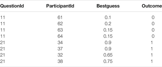
TABLE 1. Excerpt of the complete data set.
2.2 Embed Brier Scores into Mixed-Effects Models
Multilevel models are also known as hierarchical models and they are fitted to multilevel or hierarchical data structures [18]. Multilevel or hierarchical data structures consist of multiple units of analysis that are ordered hierarchically, and they exist in general when some units of analysis can be considered as subsets of others in a hierarchy [19]. The observations between levels in a hierarchical structure are considered independent, but dependent within levels as they belong to the same subpopulation [20]. If we consider the above discussed experiment where several experts are predicting probabilities of multiple events, the expert data represents a hierarchical data structure with two levels for the experts and questions. Therefore, the probability predictions can be correlated due to the common grouping effects of experts and questions.
Mixed-effects models can represent potential covariance or correlation structures induced due to the groupings of data by associating common random effects to observations that share the same levels of grouping factors { [21], chap. 1}. Random effects impose observations that share the same levels of grouping to have the same intercept and/or slope [22]. Therefore, we intend to compute expert Brier scores using a mixed-effects model that includes question effects as random effects. Hence, the estimated standard errors of expert Brier scores from the fitted mixed-effects models can be expected to be more accurate than the typically computed standard error estimates ignoring potential correlated probability predictions due to the effects of common questions.
It is important to note that linear mixed-effects models generalize best when they include the maximal random effects structure justified by the design [23]. Here, we only applies random intercepts to incorporate questions’ effects assuming that effects of questions’ difficulty on predictions is same for all the participants in the analysis. If the differential impact of questions’ difficulty on the predictions of different participants can be assessed, then the random slopes for questions’ effects together with random intercepts can also be introduced into the model to enhance the accuracy of standard error estimates in future analyses.
The correlations between probability predictions due to the question effects can be included into the above model either as fixed effects or as random effects. If we include them as fixed effects, the model needs to estimate the effects of each and every level of the questions as separate parameters in the model. These parameters will behave as nuisance parameters and avoid estimating
where
2.3 The Analysis of Standard Errors
It follows from the discussion in Section 1.3 that the typical and linear fixed-effects model (Eq. 3) based Brier scores will be identical for the participants (we verified this claim for our data, not shown here). If we consider the estimation of standard errors of Brier scores, then potential correlations between probability predictions due to the effects of common questions have not been considered in both methods. Therefore, the independence assumption of random errors
Pinheiro and Bates [21] discussed fitting linear fixed-effects models with both constant and non-constant within-group errors using the generalized least squares estimation method. Therefore, we considered fitting the above discussed linear fixed-effects model together with the following extended linear fixed-effects model with non-constant variances of within-participant errors.
where the difference from the model in Eq. 3 is to assume that
We used the “gls (generalized least squares)” function of the “nlme (Linear and Nonlinear Mixed Effects Models)” package [24] of the R software package to fit the above two linear models. We observed that the standard error estimates of Brier scores from the Linear_nc model are identical to the corresponding typically computed estimates. Furthermore, the constant variance assumption of errors in Linear_c model resulted in equal standard error estimates of Brier scores due to the pooled variance estimation discussed above. Therefore, we consider the practical importance of identifying a model that produces Brier scores and their standard error estimates that are similar to the corresponding estimates from the typical computation of Brier scores and focus on possible improvements afterward. Linear_nc model produces similar estimates of Brier scores and their standard errors to the typically computed values.
The reason for choosing the generalized least squares (GLS) estimation method in the model in Eq. 5 over the ordinary least squares (OLS) estimation method in the model in Eq. 3 was discussed above. It is a well-known fact that the maximum likelihood and ANOVA based OLS estimates are equivalent under the assumptions of the linear regression models. Even though, we are moving from the OLS estimation to the GLS estimation under the non-constant error variances within participants, the diagonal covariance structure assumption still remains. According to [25], altering the covariance structure of a parametric model alters the estimated standard errors of the model’s estimated parameters. Therefore, the maximum likelihood estimates of the standard errors of individual participants’ Brier scores obtained from the typical computation based on the deviations of observations
2.4 Imputation
We now briefly describe candidate imputation methods. The mean imputation method is one of the default methods used in major statistical packages together with the case deletion method [26]. The mean imputation method imputes missing values by substituting the missing values of a given variable by the mean value of the observed values of that variable [17]. According to [27], the mean imputation method needs to satisfy the MCAR (Missing Completely at Random) assumption to obtain unbiased results. We consider the mean imputation as one of the imputation methods in this analysis.
Next, we consider regression imputation [26]. This method fits a regression equation considering the observed values of a given variable with missing values as the response variable and all the other relevant variables in the data set as predictor variables. Then, the predicted values from the fitted regression equation are used to impute missing values [27]. According to [28], this method provides a sound basis for many of the modern missing value estimating methods. The results are unbiased if the MCAR or MAR (Missing at Random) conditions hold [27]. As mentioned in Section 1.4, we intend to make statistical corrections for missing values using mixed-effects models. Mixed-effects models will be useful to better reflect the data by incorporating potential correlations between probability predictions. Hence, the resulting imputed values for the missing probability predictions can be more accurate. Thus, we will use an appropriate mixed-effects models as the imputation model in regression imputation.
The above discussed imputation methods only perform single imputations of missing values [29] discussed the importance of considering the uncertainty of an imputation process by repeating the process multiple times. Therefore, it is also of interest to apply suitable advanced missing-value estimation methods that employ iterative procedures to take into account the underlying uncertainty of the imputation process. [16,28] noted that multiple imputation, full information maximum likelihood, and EM (Expectation-Maximization) algorithm are commonly used advanced missing-value estimation methods.
Furthermore, the Markov-chain imputation method is also used in practice [27]. However, the Markov-chain imputation method is usually applied to longitudinal (or repeated measures) data [27] which does not fit our context of computing experts’ Brier scores. The full information maximum likelihood is a model-based missing data estimation method commonly applied in structural equation modeling [16]. It is a general and convenient framework to conduct statistical analyses in several multivariate procedures including factor analysis, multivariate regression analysis, discriminant analysis, canonical analysis, and so on [30]. Therefore, this method is also not applicable in our context.
Even though the EM algorithm can be applied in this context, we found no applications of the EM in the context of estimating parameters of fixed effects of linear mixed-effects models with missing values.
Hence, in this study, we restricted our attention to a hand-full of methods to impute missing probability predictions in computing experts’ Brier scores: the mean imputation, the regression imputation, and the multiple imputation with mixed-effects models.
The same intelligence game data set was used (as in the previous section of the analysis) and a complete subset of predictions without missing values was selected from the third year data of the forecasting tournament (Section 2.1). A simulation study was performed by randomly introducing some selected percentages of missing values into the “Bestguess” variable of probability predictions. Once the missing values are estimated using the selected imputation methods, Brier scores were recomputed with the imputed missing values. The analysis was repeated 1,000 times at each percentage of missing values and the mean error of computing Brier scores over 1,000 repeats;
The exact missing data mechanism of that contributes to missing predictions is unknown in the context of computing expert Brier scores. Therefore, we assumed two scenarios, i) missing data occur completely at random and ii) missing data occurring with probability conditional on the levels of difficulty of questions. We also considered two different ways of introducing the selected percentages of missing values into the probability predictions made by participants in the analysis. In the first case, we introduced the selected percentages of missing values directly into the overall set of predictions made by participants to represent a context in which different participants may have different numbers of missing predictions (unbalanced missingness). Secondly, we introduced the selected percentages of missing values equally into the predictions made by each participant individually (balanced missingness). The results of the analysis are summarized in Section 3.2 below.
The original data set of the third year second round best guess probability predictions that was used to obtain a sample of complete set of predictions follows the same structure as shown in the above analysis of computing standard errors of Brier scores in Table 2. The selected subset includes data from six participants answering 31 questions each. Therefore, the data contain a total of 186 probability predictions. Considering the total number of 186 predictions for introducing random missing values directly into the overall set of predictions made by participants and 31 predictions for introducing random missing values for each individual participant, we considered 10% as a reasonably small percentage of missing values and 25% as a reasonably large percentage of missing values. Therefore, we reduced the scope of the analysis to introduce 10 and 25% missing values.
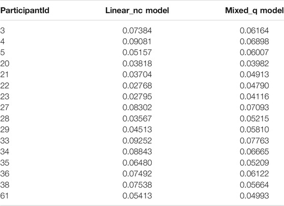
TABLE 2. Standard error estimates of participants’ Brier scores.
The purpose of using the third year second round data of the intelligence game was to consider the possibility of incorporating potential correlations between probability predictions due to the effects of not only the common questions but also the common groupings of participants into the analysis. It was observed that the standard error estimates of participants’ Brier scores of the selected complete set of predictions were not varied considerably between participants as in the analysis of the previous section. Therefore, we relaxed the need of using non-constant within group variances of predictions for participants and looked into fitting a mixed-effects model with non-nested random effects for both questions and groups in the analysis.
However, fitted mixed-effects models with random effects for groups and questions produced singular fits. There is no theoretical reason to always obtain singular fits for this model with an additional random effects for groups. It should have observed due to specific characteristics of this particular data set used in the analysis. Insufficient number of groups and inadequate number of participants within groups of the selected data can be suggested as potential reasons for this observation. In response to this issue, regression imputation and multiple imputation were carried out using the following imputation model with questions as the only random effect.
Here,
3 Results
3.1 Modeling Framework and Standard Errors
Figure 1 plots the Brier scores and standard errors using the standard and linear-model approach, and confirms that for these data, the estimates are indistinguishable, as suggested by the development of the model.
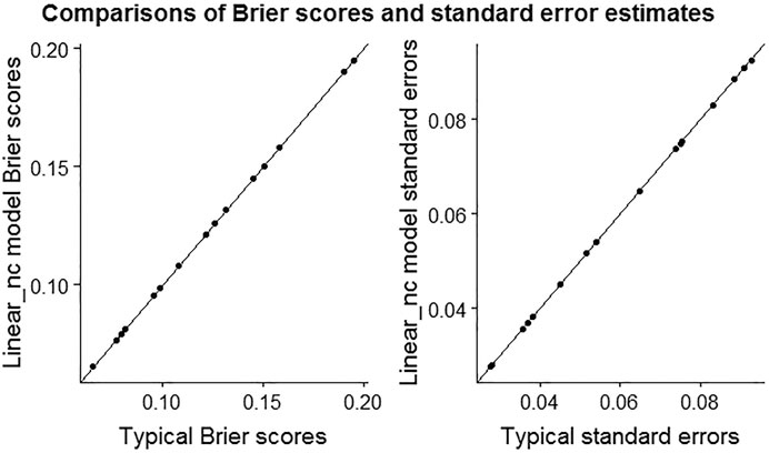
FIGURE 1. The scatter plots of Brier scores and standard error estimates from typical and Linear_nc model based computations.
It is important to note that potential correlations between probability predictions due to the effects of common questions has not been incorporated to the analysis yet in the model discussed above. Therefore, we next consider fitting the linear mixed-effects model in Eq. 4 with question effects as random effects. The random effects for questions will accommodate potential correlations between probability predictions due to the common questions in the model. It follows from above that we assume non-constant variances for random errors within participants. [21] also discussed the possibility of extending linear mixed-effects models to allow heteroscedastic or non-constant variances for within-group errors of a given stratification variable. Furthermore, there is no restriction on the grouping factor to be a fixed-effect or a random-effect in the model. Therefore, we considered participants as the stratification variable of the model. It leads to fit the following adjusted linear mixed-effects model with non-constant variances of errors within participants.
where the difference from the model four is to assume that
We expected that participant Brier scores similar to the typical computation will also be obtained from Mixed_q model for this complete set of predictions. However, we expect to improve the accuracy of the estimated standard errors of participant Brier scores from Mixed_q model. The effective sample size (
The likelihood ratio test with a very small p-value and the lower AIC and BIC values of the Mixed_q model suggest that Mixed_q model better reflects the data than the Linear_nc model as indicates in Table 3. Therefore, we conclude that the accuracy of the estimated standard errors of participants’ Brier scores are improved from the Mixed_q model compared to the typical computation of Brier scores. Figure 2 indicates that participant Brier scores are similar but the standard error estimates are different between the typical and mixed-effects model based computations, as expected. The enclosed R codes (as a Supplementary Material) show the computation procedure and the computed values of the Brier scores and their standard errors in the analysis.

TABLE 3. Comparison of the adequacy of linear and mixed-effects models.
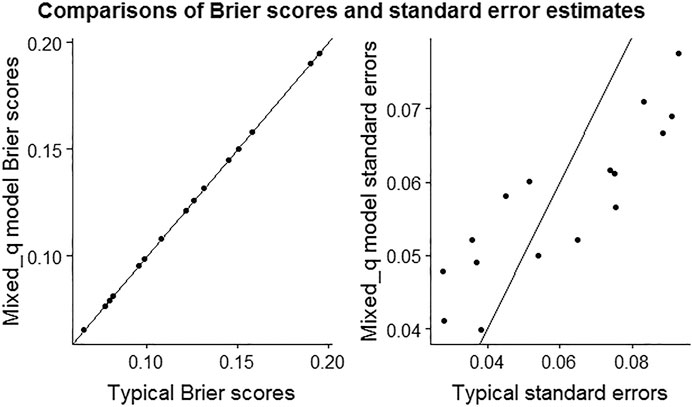
FIGURE 2. The scatter plots of Brier scores and standard error estimates from typical and Mixed_q model based computations.
3.2 The Analysis of Missing-Value Imputation
We now present the results of the imputation simulation exercise.
Figure 3 shows the estimated mean errors of computing Brier scores with 95% confidence intervals (assuming estimated errors of computing Brier scores follow normal distributions with unknown means and variances) for the mean imputed, the regression imputed, the multiple imputed and the typically computed Brier scores (ignoring missing values) under 10% overall missing values of predictions introduced completely at random. According to Figure 3, the mean error of computing Brier scores with multiple imputed missing values is the lowest and statistically different to mean error of computing Brier scores using the other imputation methods. It can also be seen that confidence intervals of other three methods overlap, implying that mean errors of computing Brier scores are not statistically different under 0.05 level of significance.

FIGURE 3. Estimated mean errors with 95% confidence intervals for computing Brier scores with 10% overall missing values introduced completely at random.
The regression imputation method with a single imputation seems to have slightly higher sample mean error, when compared to the typically computed Brier scores (ignoring missing values). We note that there is an underlying uncertainty of generating random values for imputing missing values using the suggested mixed-effects model in the regression imputation method. We take this uncertainty into account by using multiple generated values. Also note that the mean imputation method of using participants’ effect to estimate missing values can reduce the sample mean error (to some extent) when compared to that of the typically computed Brier scores. However, it failed to achieve a significant difference. Figure 4 has almost similar interpretation of results for the case of 10% individual missing values of predictions introduced completely at random.
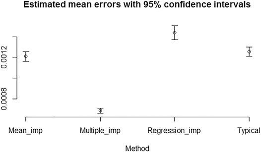
FIGURE 4. Estimated mean errors with 95% confidence intervals for computing Brier scores with 10% individual missing values introduced completely at random.
We do not focus much on the individual differences between mean errors of the mean imputation, the regression imputation, the multiple imputation, and the typical computation of missing values in this analysis. We just emphasize the fact that the mean error of multiple imputed missing values is lowest and statistically different from the mean errors calculated using the other methods. The same property holds in the case of 25% overall and individual missing values introduced completely at random.
Next, we consider introducing missing predictions not at random but conditional on the levels of difficulty of questions. Therefore, we introduced missing values with probabilities proportional to the questions’ Brier scores, representing the scenario that more difficult questions could be more likely to be skipped by participants, generating missing values. Therefore, the missing data mechanism would satisfy the not missing at random (NMAR) condition that is generally based on a non-testable assumption [29]. The use of mixed-effects models in both the regression and the multiple imputation methods with random effects for questions will incorporate the potential correlations between probability predictions caused by underlying differences between the levels of difficulty of questions into the imputation of missing values. Therefore, it may reduce (but not completely eliminate) the impact of ignoring the potential NMAR condition on the results of mean imputation method in the analysis.
Similar analysis as in the previous section has been carried out. Here, we report the result of the analysis for introducing 25% overall and individual missing predictions. Figures 5, 6 show that the mean errors of multiple imputed missing values are the lowest and statistically different from the mean errors produced by the other methods for computing Brier scores with 25% overall and individual missing values. We observed the same overall pattern of result when introducing 10% overall and individual missing predictions.
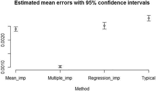
FIGURE 5. Estimated mean errors with 95% confidence intervals for computing Brier scores with 25% overall missing values introduced not at random.
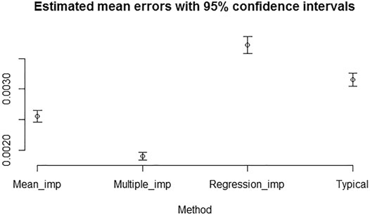
FIGURE 6. Estimated mean errors with 95% confidence intervals for computing Brier scores with 25% individual missing values introduced not at random.
4 Discussion and Conclusion
We have shown that adoption of an analysis approach that reflects the experimental design has material impacts on the outcomes of the analysis. Mixed-effects models allow the analyst to match hierarchical structures in the data-generating process, which results in a more accurate analysis.
Standard errors are key to understanding the amount of uncertainty inherent in interpreting random variables. Traditionally, standard errors have been computed for Brier scores in what amounts to a completely randomised design framework, that is, as though each expert is presented their own unique set of calibration questions. We do not know of any SEJ setup in which this assumption would be true. The implication is that the expert data reflect a hierarchical structure that is ignored in the analysis, which means that estimates may be biased and inefficient, especially if the data are unbalanced. The remedy is simple: either apply post-hoc corrections, or as we have here, adopt a model paradigm that matches the experimental design. This also allows for the possibility of estimating the magnitude of the correlation structure, via estimates of the random effects, and even (should it be of interest) formally testing the fidelity of the data to the simpler design, as we have in Table 3.
The challenge of missing data is very common in SEJ. The most popular solution seems to be case-wise deletion, which creates statistical inefficiencies and possibly biases depending on the missingness mechanism, in other words the systemic aspects of the experimental setup that lead to data missingness. Here we have demonstrated the use of several different imputation approaches to try to obtain full value from the data. There are many other possible approaches involving a range of modeling infrastructure, for example random forests, and it is easy to become bewildered. We firmly believe that doing something is better than doing nothing.
Imputation is particularly useful when expert opinions are inserted into a higher-level simulation model, pairwise or in higher dimension. As a trivial example, imagine an SEJ exercise to elicit from six experts proficient in statistics, the slope
Now, imagine that expert six provides only the intercept, so that
The deployment of imputation should be handled with considerable care and with careful scrutiny, because startling results may ensue and indeed degrade the quality of the experiment. So although we recommend the unflinching deployment of mixed-effects models methods for the analysis of SEJ experiments, our support of imputation is more nuanced.
We note that this study was performed based on a specific data set. Therefore, there is a possibility that some specific characteristics of the data set may have caused mixed-effects models or multiple imputation to work well. We did not focus on performing a simulation study to theoretically prove the ability of multiple imputation with a given mixed-effects model to perform better than the other considered methods in some specific conditions. Such an exercise would just repeat existing simulation exercises that demonstrate the importance of imputation [31–33] in general conditions.
The final consideration that arises from applying an experimental-design lens to SEJ is that of the potential efficiencies that can arise from deploying carefully designed experiments. Treating an SEJ exercise as though it had been a designed experiment yields some efficiencies, as explored in this paper, but not to the extent that would accrue from designing the SEJ experiment from the start. Experimental design as a discipline has paid considerable attention to the problem of how to most efficiently establish information within setups that reflect frail experimental units. For example, balanced incomplete block designs could present a specially selected subset of questions to a group of experts that would result in reduced effort but at a marginal cost, and indeed if expert fatigue comes into consideration it is not hard to imagine scenarios in which asking a smaller number of questions is downright advantageous.
To sum up, adoption of appropriate experimental design protocols does three things for SEJ, namely.
1) Provides better estimates of quantities of interest.
2) Provides a framework for imputation, leading to better analysis outcomes; and
3) Provides a framework for considering more efficient design of experiments, obtaining the same quality of information with less effort.
Data Availability Statement
The raw data supporting the conclusions of this article will be made available by the authors, without undue reservation.
Author Contributions
All three authors conceptualized the research question. GD developed the models, carried out the analyses and took the lead in writing the manuscript. AH and AR co-authored, reviewed and edited the manuscript.
Funding
AH and AR were supported by CEBRA at the University of Melbourne.
Conflict of Interest
The authors declare that the research was conducted in the absence of any commercial or financial relationships that could be construed as a potential conflict of interest.
Supplementary Material
The Supplementary Material for this article can be found online at: https://www.frontiersin.org/articles/10.3389/fams.2021.669546/full#supplementary-material
The R codes used to the compute Brier scores and their standard errors are enclosed herewith as a supplementary document.
Footnotes
1According to [34], the halo effect can be generally defined as a psychological phenomenon that leads to extrapolate from a general impression to unknown attributes.
References
1. Anon, . Predicting an Uncertain World. How Spooks Are Turning to Superforecasting in the Cosmic Bazaar. Economist (2021).
2. Hora, SC, Fransen, BR, Hawkins, N, and Susel, I. Median Aggregation of Distribution Functions. Decis Anal (2013) 10:279–91. doi:10.1287/deca.2013.0282
3. Baron, J, Mellers, B, Tetlock, P, Stone, E, and Ungar, L. Two Reasons to Make Aggregated Probability Forecasts More Extreme. Decis Anal (2014) 11:451–68. doi:10.1287/deca.2014.0293
4. Satopää, VA, Salikhov, M, Tetlock, PE, and Mellers, B. Bias, Information, Noise: The Bin Model of Forecasting. Management Sci (2021) doi:10.1287/mnsc.2020.3882
5. Brier, GW. Verification of Forecasts Expressed in Terms of Probability. Mon Wea Rev (1950) 78:1–3. doi:10.1175/1520-0493(1950)078<0001:vofeit>2.0.co;2
6. Candille, G, and Talagrand, O. Evaluation of Probabilistic Prediction Systems for a Scalar Variable. Q J R Meteorol Soc (2005) 131:2131–50. doi:10.1256/qj.04.71
7. Wintle, B, Mascaro, S, Fidler, F, McBride, M, Burgman, M, Flander, L, et al. The Intelligence Game: Assessing delphi Groups and Structured Question Formats. In: 2012 SECAU Security and Intelligence Congress. Perth, Western Australia: SRI Security Research Institute, Edith Cowan University (2012) p. 1–26.
8. Hanea, AM, McBride, MF, Burgman, MA, Wintle, BC, Fidler, F, Flander, L, et al. Investigate discuss estimate aggregate for structured expert judgement. Int J Forecast (2017) 33:267–79. doi:10.1016/j.ijforecast.2016.02.008
9. Finch, WH, Bolin, JE, and Kelley, K. Multilevel Modeling Using R. Boca Raton, FL: CRC Press (2016).
10. Van den Noortgate, W, Opdenakker, M-C, and Onghena, P. The Effects of Ignoring a Level in Multilevel Analysis. Sch Effectiveness Sch Improvement (2005) 16:281–303. doi:10.1080/09243450500114850
11. Hox, JJ. Multilevel Analysis: Techniques and Applications. Mahwah, N.J.: Lawrence Erlbaum Associates, 2002 (2002).
12. Blattenberger, G, and Lad, F. Separating the Brier Score into Calibration and Refinement Components: A Graphical Exposition. The Am Statistician (1985) 39:26–32. doi:10.1080/00031305.1985.10479382
13. Predd, JB, Osherson, DN, Kulkarni, SR, and Poor, HV. Aggregating Probabilistic Forecasts from Incoherent and Abstaining Experts. Decis Anal (2008) 5:177–89. doi:10.1287/deca.1080.0119
14. Merkle, EC, Steyvers, M, Mellers, B, and Tetlock, PE. Item Response Models of Probability Judgments: Application to a Geopolitical Forecasting Tournament. Decision (2016) 3:1–19. doi:10.1037/dec0000032
15. Hanea, AM, McBride, MF, Burgman, MA, and Wintle, BC. Classical Meets Modern in the Idea Protocol for Structured Expert Judgement. J Risk Res (2018) 21:417–33. doi:10.1080/13669877.2016.1215346
16. Dong, Y, and Peng, C-YJ. Principled Missing Data Methods for Researchers. SpringerPlus (2013) 2:222. doi:10.1186/2193-1801-2-222
17. Kang, H. The Prevention and Handling of the Missing Data. Korean J Anesthesiol (2013) 64:402–6. doi:10.4097/kjae.2013.64.5.402
18. Gelman, A, and Hill, J. Data Analysis Using Regression and Multilevel/hierarchical Models. New York, NY: Cambridge University Press (2006).
19. Steenbergen, MR, and Jones, BS. Modeling Multilevel Data Structures. Am J Polit Sci (2002) 46:218–37. doi:10.2307/3088424
20. Demidenko, E. Mixed Models: Theory and Applications with R. Hoboken, NJ: John Wiley & Sons (2013.).
21. Pinheiro, JC, and Bates, DM. Mixed Effects Models in S and S-PLUS. New York: Springer (2000) p. c2000.
22. Harrison, XA, Donaldson, L, Correa-Cano, ME, Evans, J, Fisher, DN, Goodwin, CED, et al. A Brief Introduction to Mixed Effects Modelling and Multi-Model Inference in Ecology. PeerJ (2018) 6:e4794. doi:10.7717/peerj.4794
23. Barr, DJ, Levy, R, Scheepers, C, and Tily, HJ. Random Effects Structure for Confirmatory Hypothesis Testing: Keep it Maximal. J Mem Lang (2013) 68:255–78. doi:10.1016/j.jml.2012.11.001
24. Pinheiro, J, Bates, D, DebRoy, S, and Sarkar, D. R Core Team (2017) Nlme: Linear and Nonlinear Mixed Effects Models. R Package Version 3.1-131 (2017) Computer software] Retrieved from https://CRAN.R-project.org/package=nlme.
25. Lange, N, and Laird, NM. The Effect of Covariance Structure on Variance Estimation in Balanced Growth-Curve Models with Random Parameters. J Am Stat Assoc (1989) 84:241–7. doi:10.1080/01621459.1989.10478761
26. Scheffer, J. Dealing with Missing Data. In: Research Letters in the Information and Mathematical Sciences, 3. Citeseer (2002) p. 153–60. https://mro.massey.ac.nz/handle/10179/4355?show=full.
27. Bennett, DA. How Can I deal with Missing Data in My Study? Aust New Zealand J Public Health (2001) 25:464–9. doi:10.1111/j.1467-842x.2001.tb00294.x
28. Graham, JW. Missing Data Analysis: Making it Work in the Real World. Annu Rev Psychol (2009) 60:549–76. doi:10.1146/annurev.psych.58.110405.085530
29. Harel, O, and Zhou, X-H. Multiple Imputation: Review of Theory, Implementation and Software. Statist Med (2007) 26:3057–77. doi:10.1002/sim.2787
30. Hox, JJ, and Bechger, TM. An Introduction to Structural Equation Modeling. Fam Sci Rev (1998) 11:354–73.
31. Janssen, KJM, Donders, ART, Harrell, FE, Vergouwe, Y, Chen, Q, Grobbee, DE, et al. Missing Covariate Data in Medical Research: to Impute Is Better Than to Ignore. J Clin Epidemiol (2010) 63:721–7. doi:10.1016/j.jclinepi.2009.12.008
32. Ambler, G, Omar, RZ, and Royston, P. A Comparison of Imputation Techniques for Handling Missing Predictor Values in a Risk Model with a Binary Outcome. Stat Methods Med Res (2007) 16:277–98. doi:10.1177/0962280206074466
33. Demirtas, H. Simulation Driven Inferences for Multiply Imputed Longitudinal Datasets. Stat Neerland (2004) 58:466–82. doi:10.1111/j.1467-9574.2004.00271.x
Keywords: hierarchical data, mixed-effects models, random effects, within-question correlations, imputation, experimental design, structured expert judgement
Citation: Dharmarathne G, Hanea A and Robinson AP (2021) Improving the Computation of Brier Scores for Evaluating Expert-Elicited Judgements. Front. Appl. Math. Stat. 7:669546. doi: 10.3389/fams.2021.669546
Received: 19 February 2021; Accepted: 26 May 2021;
Published: 10 June 2021.
Edited by:
Don Hong, Middle Tennessee State University, United StatesReviewed by:
Michael Chen, York University, CanadaVajira Manathunga, Middle Tennessee State University, United States
Copyright © 2021 Dharmarathne, Hanea and Robinson. This is an open-access article distributed under the terms of the Creative Commons Attribution License (CC BY). The use, distribution or reproduction in other forums is permitted, provided the original author(s) and the copyright owner(s) are credited and that the original publication in this journal is cited, in accordance with accepted academic practice. No use, distribution or reproduction is permitted which does not comply with these terms.
*Correspondence: Gayan Dharmarathne, c2FtZWVyYUBzdGF0LmNtYi5hYy5saw==