Multilevel Assimilation of Inverted Seismic Data With Correction for Multilevel Modeling Error

1 Introduction

Sound decision-making in petroleum reservoir management depends on provision of reliable production forecasts from petroleum reservoir models, including provision of the uncertainty in the forecasts. The reliability is increased by utilization of available data for calibration of the models. Ensemble-based data assimilation (DA) methods, using statistically correct formulations, have accordingly become popular for automated reservoir history matching [1–4].

Monte Carlo approximations play crucial roles in ensemble-based DA. Due to computational cost limitations, the ensemble size is limited to roughly one hundred. Using straightforward ensemble-based DA, the degrees of freedom of the problem would equal the ensemble size, and such an approach would result in significant Monte Carlo errors. The negative effects of Monte Carlo errors are enlarged in the presence of large amounts of data to be assimilated simultaneously, for example, inverted seismic data, resulting in underestimation of variance of the unknown parameters and, in more severe cases, even in ensemble collapse.

The most widely used treatment for Monte Carlo errors is distance-based localization. The basic assumption underlying this method is that true correlations between a parameter and a datum decrease when the distance between their respective locations increases, and disappear if the distance exceeds a critical distance. This assumption may not always hold for subsurface problems. Different correlation functions and their utilization in DA can be found in References [5–7]. A proper choice of correlation function, as well as the critical distance in particular, depends on parameter and data types as well as on other problem settings. This reduces the robustness of distance-based localization, also for problems where its basic assumption does hold.

Simply increasing the ensemble size will, of course, reduce Monte Carlo errors, but it will also increase computational cost. Utilization of a lower cost and lower fidelity model renders the possibility of increasing the ensemble size without increasing the total computational cost. The use of a lower fidelity reservoir model will however introduce modeling errors in addition to those already present in conventional fidelity simulation results. The underlying assumption when applying lower fidelity models in DA is therefore that the gain in reducing Monte Carlo errors is larger than the loss in numerical simulation accuracy. If the abovementioned additional modeling errors could be approximately accounted for, utilization of lower fidelity models would be even more attractive. DA using various types of lower fidelity models has been applied to several inverse problems, for example, within petroleum reservoir modeling [8–10] and atmospheric science [11]. Note that since lower fidelity simulations are applied to the forecast step and localization is applied to the analysis step, the two techniques can be combined, if desired.

Multilevel simulations utilize a selection of models for the same entity that constitute hierarchies in both fidelities and computational costs (multilevel models). The idea is to decrease Monte Carlo errors without increasing numerical errors too much. There are a number of ways to realize multilevel models. We choose to construct them by spatial coarsening of the conventional simulation grid to several levels of coarseness and correspondingly upscale the associated grid-based parameter functions. Multilevel data assimilation (MLDA) [12–16] utilizes multilevel simulations in the forecast step. Since inverted seismic data are given on the conventional grid (denoted as the fine grid from now on), MLDA with such data must be able to handle differences in grid levels between data and model forecasts.

Modeling errors are ubiquitous in all numerical simulations in the geosciences. In the context of a coarse-grid numerical model, three types of modeling errors can be envisioned: Type 1: the discrepancy between the physical reality and the solution obtained with a mathematical model attempting to model the physical reality; Type 2: the discrepancy between the solution obtained with that mathematical model and the model forecast from a numerical model resulting from discretization of the mathematical model; and Type 3: the discrepancy between the model forecast from that numerical model and the model forecast from a numerical model with a coarser simulation grid.

Assuming a normal distribution for the errors, a Bayesian framework for jointly accounting for Type 1 and Type 2 modeling errors in DA was presented in Reference [17]. The effect of Type 2 modeling errors on the solution to linear Gaussian inverse problems was analyzed in Reference [18]. (Neither Ref. [17] nor Ref. [18] were concerned with Type 3 modeling errors.) In this study, we quantify and approximately account for Type 3 modeling errors for each level in multilevel assimilation of spatially distributed data, such as inverted seismic data. (We will use the term multilevel modeling error (MLME) to denote this error from now on.) To this end, three computationally inexpensive approximate MLME correction schemes are developed, and their abilities to correct multilevel model forecasts for reservoir models with different types of MLME are assessed and compared to a previously proposed (also computationally inexpensive) MLME correction scheme. Additionally, we assess the performances of the different MLME-corrected model forecasts in assimilation of bulk impedance data. The posterior parameter estimates from MLDA with and without MLME correction are compared to results obtained from conventional single-level DA with localization.

The rest of this article is framed as follows. Section 2 is devoted to explaining MLDA and introducing a recently devised algorithm for it. Section 3 introduces MLME and the four proposed schemes for addressing it. Section 4 explains the reservoir models used for assessment of the performance of MLME correction schemes in MLDA. In Section 5, we describe the numerical investigations, which are followed by their results in Section 6. Finally, in Section 7, we summarize and conclude the study.

2 Multilevel Data Assimilation

The forecast step in ensemble-based DA takes the initial states and parameters as input and generates the model forecasts. In this work, the forecast step of MLDA is performed using a hierarchy of nested forward models, ${\left\{{\mathrm{ℳ}}_l\right\}}_{l=0}^L$. After sampling from the prior distribution, the ensemble of prior state vectors is divided into L sub-ensembles. Hence, each of the sub-ensembles are modeled using corresponding forward models, as seen in Figure 1, where Z is the random vector of parameters and subscripts denote the sub-ensemble number.

FIGURE 1

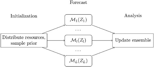
FIGURE 1. Representation of MLDA algorithms.

In order to give a description for a full cycle of MLDA of spatially distributed data, multilevel models should be discussed. Additionally, since the MLDA uses the ensemble approximations of the mean and covariance of the model forecasts, which are in different resolutions for different levels, a robust transformation scheme should be devised for converting the model forecasts from one resolution to another. These two topics will be discussed in Sections 2.1 and 2.2, respectively. They will be followed by sections on upscaling of the observation data (Section 2.3) and formulation of multilevel statistics for mean and covariance of the model forecasts (Section 2.4). Afterward, a description of a recently devised method for MLDA of spatially distributed data, which will be used in our numerical experiments, is given in Section 2.5.

2.1 Multilevel Models

Let ${\left\{{\mathrm{ℳ}}_l\right\}}_{l=0}^L$ be a set of deterministic models, where the accuracy and computational cost increase with an increase in l. Accordingly, they will form hierarchies of both accuracy and cost. One can think of several schemes to devise the hierarchy including but not limited to coarsening the spatial grid of the forward model together with upscaling the associated parameters, coarsening the temporal grid of the forward model, and relaxing the convergence criteria in the iterative linear solvers. All of these methods reduce the computational cost of the models and increase their numerical error. Coarsening the spatial grid and upscaling the associated parameters are chosen for the current work. The techniques presented in this work are however robust enough so that with minor manipulations, they can be used for other lower fidelity models.

As for coarsening the grid of the forward models, the authors of Reference [15] proposed a robust technique, which was also used in Reference [16]. This technique occurs in a sequence of steps. In each step, neighboring cells of the grid at the previous step are merged into a coarser cell, unless they are to be kept fine deliberately. A representation of the grid coarsening process for an $8\times 8$ sample grid can be found in Figure 2. As it can be seen in the figure, coarsening has occurred in a uniform manner across both directions, except for the vicinity of two opposite corners, where the grid cells are kept in fine scale to boost the local numerical accuracy around the two wells, producer (P) and injector (I).

FIGURE 2

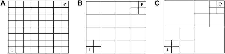
FIGURE 2. Grid coarsening proposed by [15] performed on an 8 × 8 grid (A) finest level and (B, C) coarser levels.

The parameters associated with the grid are upscaled in such a way that the physics of the problem do not change drastically. Upscaling of the parameters will be further discussed in Section 4.

2.2 Transformation of Model Forecasts

The discrepancy in coarseness of the multilevel grids results in the spatially distributed model forecasts to be in different resolutions for different levels. Therefore, in order to be able to compute the multilevel sample statistics of the model forecast, a robust transformation scheme should be devised for converting a model forecast from the resolution at one level to another.

In the problem at hand, transformation of the model forecast requires either upscaling or downscaling. To this end, a standard volume-weighted arithmetic averaging technique is used. Accordingly, we define a set of linear transformations, $\left\{U_p^q:{ℝ}^{S_p}\mapsto {ℝ}^{S_q}|1\le p,q\le L\right\}$, where $S_p$ and $S_q$ denote the dimension of the model forecast vector at arbitrary levels p and q, respectively, and $U_p^q$ transforms the model forecast vector from level p to be compatible with level q.

Figure 3 gives two examples of transformation of a spatially distributed model forecast, one from a coarser grid to a finer grid and one vice versa. Each model forecast component is represented in its corresponding spatial grid cell.

FIGURE 3

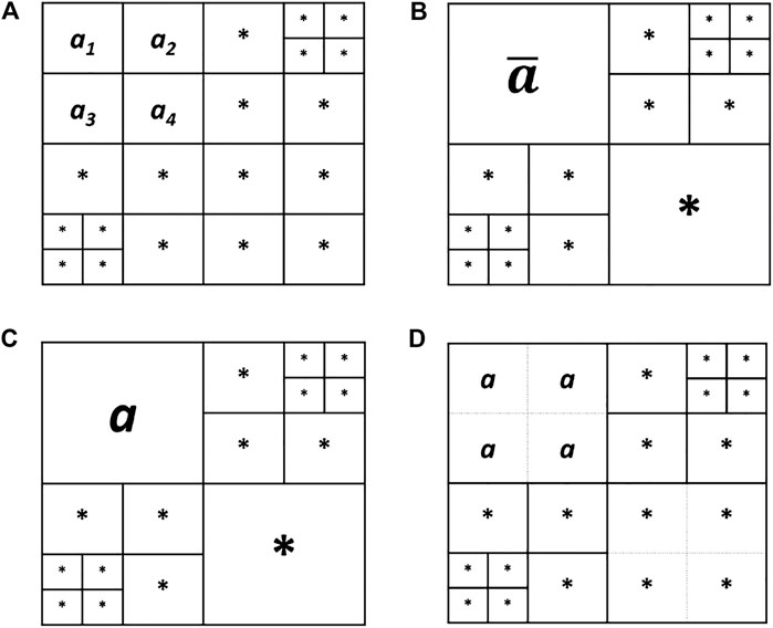
FIGURE 3. Transformation of model forecast between two levels p (finer) and q (coarser) (A) model forecast in resolution of level p, (B) transformation of model forecast from resolution of level p to the resolution of level q, (C) model forecast in resolution of level q, and (D) transformation of model forecast from resolution of level q to the resolution of level p.

As can be seen in Figure 3, in the upscaling procedure, the arbitrarily named model forecast components ${\left\{a_i\right\}}_{i=1}^4$ in the northwest zone from the finer grid (p) are averaged to form their corresponding model forecast component, $\overline{a}$, in the coarsened grid. Similar procedure has been performed for the rest of model forecast components, shown by *. In the downscaling procedure, on the other hand, the model forecast components in the coarse grid are simply copied to their corresponding components of the finer grid.

2.3 Upscaling of Observation Data

As part of the DA process, the mismatch between the model forecasts and observation data is to be calculated. Here, it is assumed that inverted seismic data are given in the resolution of the finest simulation grid. Accordingly, for each of the levels, either the observation data should be upscaled to the resolution of model forecast or the model forecast should be downscaled to the resolution of the observation data. In this study, we take the former approach. Since the observation data are in the resolution of the finest model, using the same transformation functions as those designed for model forecasts on the fine observation data will result in upscaling of observation data into the preferred resolution.

2.4 Multilevel Statistics

Assuming we have approximations of the model forecasts, Y, being a function of the unknown parameter vector Z in several levels, a statistically correct scheme for approximation of multilevel statistics for Y is required. As for MLDA, the first two central moments of the model forecast are of foremost interest. Accordingly, formulations for these multilevel statistics are proposed.

Assuming the model with the highest fidelity, ${\mathrm{ℳ}}_L$, to be exact, the authors of Reference [13] proposed an unbiased formulation for approximation of multilevel statistics for DA under certain conditions. Under these sets of conditions, the proposed method outperformed its alternatives [12]. For reservoir problems, however these conditions typically do not hold, and another formulation based on Bayesian model averaging (BMA) was proposed [12]. In this formulation, the statistics are computed based on reliability weights $w_l$ for each of the levels l. This formulation is, by definition, a biased scheme for computation of multilevel moments; however, it will be a useful technique for problems in which variance error dominates bias, which is often the case for petroleum reservoir problems [12]. Using this formulation and transformations of the forecast, the authors of Reference [16] proposed a formulation of multilevel statistics for spatially distributed model forecasts, which is used in the current work. According to this scheme, the multilevel mean of the model forecast at level l is given as follows:

$E_{ML}\left(Y_l\right)={\displaystyle \sum }_{k=1}^L{w}_k{U}_k^{l}E\left(Y_k\right),(1)$

where $E\left(Y_k\right)$ denotes the sample mean of the model forecast at level k. Using the law of total variance, the multilevel approximation of covariance of the model forecast at level l is formulated as follows:

$C_{\text{ML}}\left(Y_l\right)={\displaystyle \sum }_{k=1}^L{w}_k\left\{C\left(U_k^l{Y}_k\right)+\left(E\left(U_k^l{Y}_k\right)-E_{ML}\left(Y_l\right)\right){\left(E\left(U_k^l{Y}_k\right)-E_{ML}\left(Y_l\right)\right)}^T\right\}.(2)$

In addition, the parameter forecast cross-covariance can be written as follows:

${\text{C}}_{\text{ML}}\left(Z,Y_l\right)={\displaystyle \sum }_{k=1}^L{w}_k\text{C}\left(Z_k,U_k^l{Y}_k\right).(3)$

Using these ML moments enables us to utilize the classic DA formulations for updating the ensemble as will be presented in Section 2.5.

2.5 Multilevel Hybrid Ensemble Smoother

Utilizing statistics given by Eqs. 1–3, the authors of Reference [16] formulated an MLDA algorithm that rendered the possibility of assimilation of spatially distributed data, for example, inverted seismic data, in a multilevel manner. This DA algorithm was called multilevel hybrid ensemble smoother (MLHES). In this work, we briefly explain MLHES and utilize it in our numerical experiments. An iterative version of MLHES has also been developed¹.

Initially, a total of $N_t$ realizations from the prior random parameter vector $Z^{pr}$ are generated and divided into L sub-ensembles, that is, $Z_l^{pr}$, $1\le l\le L$. Note that, regardless of l, all $Z_l^{pr}$ are on the fine scale and the subscript denotes the model where they are used. Accordingly, prior realization j in sub-ensemble l, where $1\le j\le N_l$ and $1\le l\le L$, is called $z_{l,j}^{pr}$. Hence, there are $N_l$ ensemble members in sub-ensemble l. Likewise, the model forecast pertaining to simulation of $z_{l,j}^{pr}$ by the forward model ${\mathrm{ℳ}}_l$ is named ${\widehat{y}}_{l,j}$ and is given by

${\widehat{y}}_{l,j}={\mathrm{ℳ}}_l\left(z_{l,j}^{pr}\right).(4)$

The correction for MLME then would be performed as

$y_{l,j}={\widehat{y}}_{l,j}+{\epsilon }_{l,\times }\left(z_{l,j}^{pr}\right),(5)$

where $y_{l,j}$ is the model forecast ${\widehat{y}}_{l,j}$ corrected for its MLME and ${\epsilon }_{l,\times }$ is the generic term for correction of MLME. In Reference [16], the authors utilized the mean bias correction for addressing the MLME. This correction scheme is one of the MLME correction schemes investigated in this work and will be explained and discussed in more detail in Section 3.

After MLME correction, there will be a separate analysis step for each of the levels. The updated parameter vector of an arbitrary ensemble member is given by

$z_{l,j}^a=z_{l,j}^{pr}+K_l\left(d_{l,j}-y_{l,j}\right),(6)$

where the observation data realization, $d_{l,j}$, is a random pick from $\mathbb{N}\left(U_L^l{\mu }_D,U_L^l{\mathrm{ℂ}}_D{U}_L^{lT}\right)$, and ${\mu }_D$ and ${\mathrm{ℂ}}_D$ are the original observation data mean and observation data error covariance in the finest level, respectively. The level-specific Kalman gain, $K_l$, is then given as

$K_l=C_{\text{ML}}\left(Z,Y_l\right){\left(C_{\text{ML}}\left(Y_l\right)+U_L^l{ℂ}_D{\left(U_L^l\right)}^T\right)}^{-1},(7)$

where the multilevel statistics $C_{\text{ML}}\left(Y_l\right)$ and $C_{\text{ML}}\left(Z,Y_l\right)$ are given by Eqs. 2 and 3, respectively.

After the analysis step, the estimates of mean and covariance of the posterior parameter field are computed based on a pool composed of all realizations $z_{l,j}^a$ at all the levels as follows:

$E\left(Z^a\right)=\frac{1}{N_t}{\displaystyle \sum }_{l=1}^L{\displaystyle \sum }_{j=1}^{N_l}{z}_{l,j}^a(8)$

$C\left(Z^a\right)=\frac{1}{N_t-1}{\displaystyle \sum }_{l=1}^L{\displaystyle \sum }_{j=1}^{N_l}\left(z_{l,j}^a-E\left(Z^a\right)\right){\left(z_{l,j}^a-E\left(Z^a\right)\right)}^T(9)$

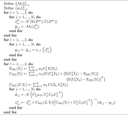
A pseudo-code of MLHES is presented in Appendix 1.

3 Multilevel Modeling Error

Let R denote some spatially varying physical property, and let W denote the forecast of a mathematical model attempting to model R. Furthermore, let $W_l$ denote the forecast of that mathematical model discretized at an arbitrarily selected level, l, and let $x_{l,n}$ denote the location of an arbitrarily selected point in the simulation grid at that level. The total modeling error in $W_l\left(x_{l,n}\right)$ when attempting to model $R\left(x_{l,n}\right)$ is then

${\varphi }_l\left(x_{l,n}\right)=R\left(x_{l,n}\right)-W_l\left(x_{l,n}\right),(10)$

which can be rewritten as

${\varphi }_l\left(x_{l,n}\right)=\left(R\left(x_{l,n}\right)-W\left(x_{l,n}\right)\right)+\left(W\left(x_{l,n}\right)-W_L\left(x_{l,n}\right)\right)+\left(W_L\left(x_{l,n}\right)-W_l\left(x_{l,n}\right)\right).(11)$

The first term on the right-hand side of Eq. 11 represents the error in the mathematical model’s forecast of physical reality, and the second term represents the discretization error when simulating with a numerical model on the fine grid. We will consider the last term, which represents the error due to numerical simulation on the level-l grid, instead of on the fine grid.

The expression $W_L\left(x_{l,n}\right)$ is precise only if $x_{l,n}$ coincides with a point in the simulation grid at level L, which will not be the case for the grid-coarsening procedure applied in the current work. To make this expression precise, we utilize the linear transformations defined in Section 2.2, and let $W_L\left(x_{l,n}\right)\stackrel{\text{def}}{=}{\left(U_L^l{W}_L\left(x_L\right)\right)}_n$. We then define component n of the multilevel modeling error (MLME) as

${\zeta }_{l,n}={\left(U_L^l{W}_L\left(x_L\right)\right)}_n-W_l\left(x_{l,n}\right),(12)$

and develop techniques for estimating ${\zeta }_l={\left({\zeta }_{l,1}\dots {\zeta }_{l,G_l}\right)}^T$ in model forecasts and approximately correcting for the MLME before assimilating data.

3.1 Multilevel Modeling Error Correction

Assuming fine model forecasts to be sufficiently accurate, ideally, the model forecasts at each level should be upscaled fine model forecasts to the resolution of that level, that is, the correction in Eq. 5 should be ${\epsilon }_{l,\times }={\zeta }_l$, but due to computational limits, this is not a possibility. Accordingly, we try to approximate ${\zeta }_l$ using the discrepancies between the model forecasts at level l and the finest level, L. This will be done using the ensemble itself without any additional simulations.

The techniques developed here are therefore computationally cheap adjunctions which can be added to many MLDA algorithms with minor modifications. The four schemes formulated and investigated in this work are named as mean bias correction (MB), stochastic correction (ST), deterministic correction (DE), and telescopic correction (TE).

Figure 4A depicts general formation of the sub-ensembles from the prior ensemble for Z. The realizations in each sub-ensemble are put in the same line as the forward model that is used for their simulation; consider each of the unit cells in the rows as a realization of the prior and each row as a sub-ensemble. Figures 4B–D describe the requirements on prior realizations for different MLME correction schemes; if parts of two sub-ensembles are of the same color, those realizations are shared between those sub-ensembles and are to be simulated using both corresponding forward models.

FIGURE 4

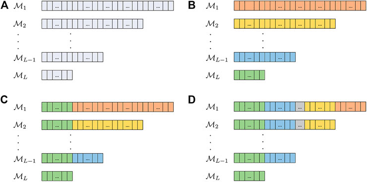
FIGURE 4. (A) Division of the prior ensemble for Z into L sub-ensembles, (B) mean bias Correction prior setting, (C) stochastic and deterministic corrections prior settings, and (D) telescopic correction prior setting.

3.1.1 Mean Bias Correction

This technique was used in Reference [12] for correction of the production data for their mean bias. There, the correction was formulated as

${\epsilon }_{l,MB,P}=E\left(Y_L\right)-E\left(Y_l\right),(13)$

where ${\epsilon }_{l,MB,P}$ is the mean bias correction term for production data. Here, we generalize this correction to be used also for spatially distributed data. Accordingly, ${\epsilon }_{l,MB}$ is defined as

${\epsilon }_{l,MB}=U_L^{l}E\left(Y_L\right)-E\left(Y_l\right),(14)$

where E(Y_L) and E(Y_l) are sample means of the model forecasts at levels L and l, respectively. Using this correction, the mean of the corrected forecast at every level would be equal to the upscaled mean of the forecast given by the most accurate (finest) model.

As can be seen in Figure 4B, in mean bias correction, as opposed to the rest of MLME correction schemes, the prior realizations are run on each of the forward models without any requirement to be run by other forward models.

3.1.2 Stochastic Correction

Simulating the sub-ensemble ${\left\{z_{l,j}^{pr}\right\}}_{j=1}^{N_L}$ using all the forward models, we can calculate ${\zeta }_l$ for those realizations as follows:

${\zeta }_l\left(z_{l,j}^{pr}\right)=U_L^l{\mathrm{ℳ}}_L\left(z_{l,j}^{pr}\right)-{\mathrm{ℳ}}_l\left(z_{l,j}^{pr}\right).(15)$

In the stochastic formulation, assuming a normal distribution for ${\zeta }_l$, the realization of correction term is formulated as

${\epsilon }_{l,ST}\sim \mathcal{N}\left(E\left({\zeta }_l\right),C\left({\zeta }_l\right)\right),(16)$

where $E\left({\zeta }_l\right)$ and $C\left({\zeta }_l\right)$ are the sample mean and covariance of realizations of ${\zeta }_l$, respectively. As the ensemble size is often relatively small in comparison to the parameter vector size, the distribution defined in Eq. 16 would not cover the full span of the probability space for ${\zeta }_l$. The realizations of ${\epsilon }_{l,ST}$, accordingly, would be in the sub-space spanned by the ensemble ${\left\{{\zeta }_l\left(z_{l,j}^{pr}\right)\right\}}_{j=1}^{N_L}$

As seen in Figure 4C and Eq. 15, this correction scheme requires the realizations at sub-ensemble L to be simulated using all the forward models.

3.1.3 Deterministic Correction

Assume that ${\zeta }_l$ is a continuous function of Z. Furthermore, we assume local linearity for ${\zeta }_l$ and write the first two terms of its Taylor expansion around the population expectation of the parameter vector, $\mathbb{E}\left(Z\right)$ as

${\zeta }_l\left(Z\right)\approx {\zeta }_l\left(\mathbb{E}\left(Z\right)\right)+\frac{\partial {\zeta }_l}{\partial Z}{|}_{\mathbb{E}\left(Z\right)}\left(Z-\mathbb{E}\left(Z\right)\right).(17)$

Under linearity assumption, we would have

${\zeta }_l\left(\mathbb{E}\left(Z\right)\right)\approx \mathbb{E}\left({\zeta }_l\left(Z\right)\right).(18)$

To calculate the Jacobian of ${\zeta }_l$, we use another approximation. Writing Stein’s lemma gives,

$\mathrm{ℂ}\left({\zeta }_l,Z\right)=\mathbb{E}\left(\frac{\partial {\zeta }_l}{\partial Z}\right)\mathrm{ℂ}\left(Z\right),(19)$

where $\mathrm{ℂ}\left(Z\right)$ and $\mathrm{ℂ}\left({\zeta }_l,Z\right)$ are covariance of Z and cross-covariance between ${\zeta }_l$ and Z, respectively. Rearranging gives

$\mathbb{E}\left(\frac{\partial {\zeta }_l}{\partial Z}\right)=\mathrm{ℂ}\left({\zeta }_l,Z\right)\mathrm{ℂ}{\left(Z\right)}^{-1},(20)$

and the local linearity assumption gives the approximation

$\frac{\partial {\zeta }_l}{\partial Z}{|}_{\mathbb{E}\left(Z\right)}\approx \mathbb{E}\left(\frac{\partial {\zeta }_l}{\partial Z}\right).(21)$

We would then use the ensemble for approximation of both mean and Jacobian of ${\zeta }_l$ and use them for formulating the deterministic correction as follows:

${\epsilon }_{l,DE}\left(E\left(Z\right)\right)\approx E\left({\zeta }_l\right),(22)$

$\frac{\partial {\epsilon }_{l,DE}}{\partial Z}{|}_{E\left(Z\right)}\approx C({\zeta }_l,Z)C{\left(Z\right)}^{+},(23)$

${\epsilon }_{l,DE}\left(Z\right)={\epsilon }_{l,DE}\left(E\left(Z\right)\right)+\frac{\partial {\epsilon }_{l,DE}}{\partial Z}{|}_{E\left(Z\right)}\left(Z-E\left(Z\right)\right),(24)$

where the superscript $+$ in Eq. 23 denotes the Moore–Penrose pseudo-inverse. As shown in Figure 4C, in deterministic correction, as in stochastic correction, the realizations in the sub-ensemble L are to be simulated using all the forward models.

3.1.4 Telescopic Correction

This scheme utilizes the idea in deterministic correction in a telescopic manner so that it can benefit from the multilevel structure of the problem. The MLME can be written as

${\zeta }_l\left(Z\right)=U_L^l{\mathrm{ℳ}}_L\left(Z\right)-{\mathrm{ℳ}}_l\left(Z\right)={\displaystyle \sum }_{k=l}^{L-1}{U}_k^l\left(U_{k+1}^k{\mathrm{ℳ}}_{k+1}\left(Z\right)-{\mathrm{ℳ}}_k\left(Z\right)\right),(25)$

and Eq. 25 holds because all the transformations are linear and from a finer level to a coarser level. Accordingly, we can write

${\zeta }_l\left(Z\right)={\displaystyle \sum }_{k=l}^{L-1}{U}_k^l{e}_k,(26)$

where

$e_k\left(Z\right)=U_{k+1}^k{\mathrm{ℳ}}_{k+1}\left(Z\right)-{\mathrm{ℳ}}_k\left(Z\right).(27)$

This reformulation of the error term renders the possibility to approximate ${\zeta }_l$ via a summation of smaller error terms, which are approximated based on bigger ensembles. Hence, using the idea in deterministic correction for level-wise errors, $e_k$, one can write

$e_k\left(Z\right)\approx E\left(e_k\right)+C\left(e_k,Z_k\right)C{\left(Z_k\right)}^{+}\left(Z-E\left(Z_k\right)\right),(28)$

where $E\left(e_k\right)$ is the sample mean of the partial error, $C\left(e_k,Z_k\right)$ is the sample cross-covariance of ${\zeta }_l$ and Z, $C\left(Z_k\right)$ is the sample covariance of the parameter vector, and $E\left(Z_k\right)$ is the sample mean of the parameter vector, all based on the realizations in sub-ensemble k. The telescopic correction term then is

${\epsilon }_{l,TE}\left(Z\right)={\displaystyle \sum }_{k=l}^{L-1}{U}_k^l\left(E\left(e_k\right)+C\left(e_k,Z_k\right)C{\left(Z_k\right)}^{+}\left(Z-E\left(Z_k\right)\right)\right).(29)$

The idea here is that even though the errors in approximation aggregate in the summation in Eq. 26, the increase in the ensemble size would reduce Monte Carlo errors and the approximation of ${\zeta }_l$ would be more accurate, and overall, it would help to account better for the MLME.

In order to be able to perform this correction, a nested structure in the prior realizations is necessary. In other words, as seen in Figure 4D, all the realizations simulated by a forward model should also be computed using all the less accurate forward models than that model.

4 Test Models

We are interested in assessing the quality of MLME correction schemes in reservoir history matching of inverted seismic data using MLHES. In accordance with it, three different reservoir models are considered. These reservoir models have some shared properties. They are two-dimensional, with $64\times 64$ Cartesian grids, two wells in the opposite corners, an injector in the northeast corner, and a producer in the southwest corner. Compressible two-phase flow (oil and water), no-flow boundary conditions, and standard equations for capillary pressure and relative permeability are considered. A description of the other shared general properties of the reservoir models is given in Table 1. As the seismic vintages are different in each experiment, they are discussed separately in Sections 5.1–5.3.

TABLE 1

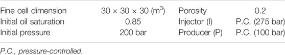
TABLE 1. Shared properties of the reservoir models.

In each of the reservoir models used in this work, the general structure is modified with the aim of increasing the MLME. These reservoir models are explained separately in Sections 4.1–4.3, and samples from the prior distribution of Z for each of the reservoir models can be found in Figure 5.

FIGURE 5

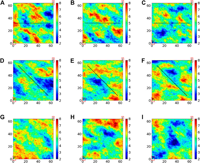
FIGURE 5. Samples from the prior distributions for log permeability for the three experiments, (A)–(C) Experiment I, (D)–(F) Experiment II, and (G)–(I) Experiment III.

The forward models used for forecast ${\left\{\mathrm{ℳ}\right\}}_{l=1}^L$ each consists of two segments. A reservoir flow model is used to predict the state variables in time, and a petro-elastic model is utilized for computing the elastic rock properties from parameters and predicted state variables.

The flow segment of the forward models is performed using Eclipse 100 [19]. Coarsening the grid is done by using the Eclipse keyword COARSEN, which merges groups of predefined neighboring cells to form a coarser grid. The upscaling of permeabilities is performed using pore-volume–weighted arithmetic averaging, and transmissibilities between two neighboring coarse cells in each direction are calculated based on harmonic averaging in that direction and summing it in other directions [19]. As for the petro-elastic segment of the forward model, an in-house model based on standard rock physics [20], [21, Report 1] was used.

4.1 Reservoir Model I

A nonpermeable fault has been added to the field with its normal vector pointing north, its eastern most point 4 grid cells away from the east side of the field, and its western most point 4 grid cells away from the west side of the field. From Figures 5A–C, it is clear that flow from the injector to the producer has to pass through one of the narrow openings at the ends of the fault. Hence, there will be strong variations in the solution variables in these regions. Grid coarsening is therefore expected to produce stronger MLME for this example than for a similar example, but where no fault was present.

4.2 Reservoir Model II

An oblique fault stretching from 8 grid cells away from the northwest corner to 8 grid cells away from the southeast corner is added to the general reservoir model structure. In addition to the complexities similar to those associated with Reservoir Model I, as can be seen in Figure 6, the coarsening scheme in the presence of such a fault, which will be discussed in Section 5.2, results in some permeability values that are located on one side of the fault in the fine grid to contribute to an upscaled permeability value located on the other side of the fault in the coarsened grid. This introduces another type of MLME to the model.

FIGURE 6

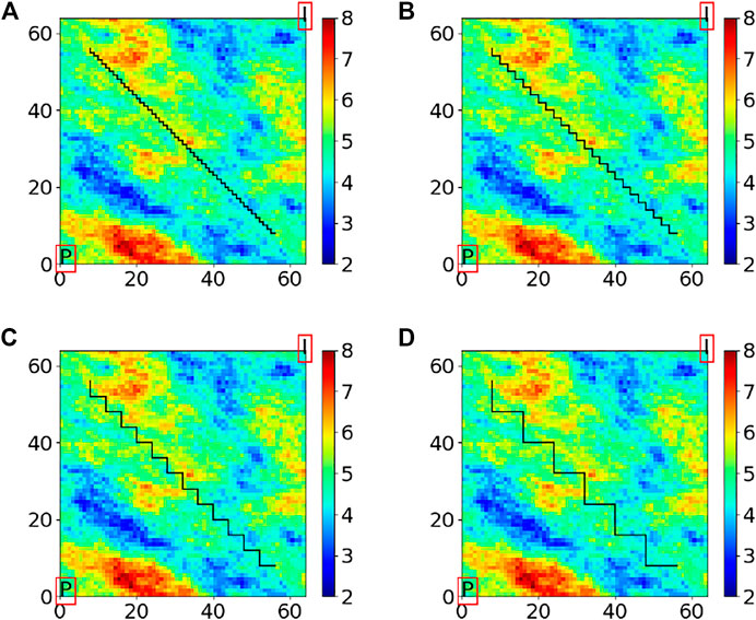
FIGURE 6. Approximation of the fault for simulations, (A) original fault and (B–D) approximations at coarser levels.

4.3 Reservoir Model III

This reservoir model uses the general structure of the models without addition of faults and is used for investigation of a different type of MLME, which is formed by simplifying the grid coarsening scheme.

5 Numerical Investigation

In order to assess the quality of the MLME correction schemes presented in this work, three experiments are conducted. The experiments are performed on the reservoir models discussed in Section 4.

The observation data are two sets of time-lapse bulk impedance data taken based on a baseline (day zero of production) and two vintages, which are different for each experiment and will be mentioned separately. These observation data are generated using the results of simulation from a random draw of the prior distribution. As the inverted seismic data are spatially correlated, we use a correlated covariance matrix for the data error. In doing so, a variogram with the specifications given in Table 2 is considered. The marginal standard deviation of each observation value is given as

$\sigma =r\text{max}\left\{\left|D\right|,T\right\},(30)$

where $r=0.1$, D is the value of observation data at a certain location, and T is a threshold put to avoid too much certainty in the observation data whose absolute value is very small. This threshold is defined as the 1st smallest percentile of the absolute value of the observation data.

TABLE 2

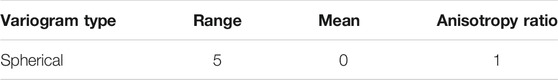
TABLE 2. Variogram used for observation data error; the unit for range is grid cells.

For each numerical experiment, we will compare plots of results (mean and variance fields) obtained with five versions of the MLHES to those obtained with ES with distance-based localization (ES-LOC). The five versions are MLHES with mean bias correction (MLHES-MB), MLHES with stochastic correction (MLHES-ST), MLHES with deterministic correction (MLHES-DE), MLHES with telescopic correction (MLHES-TE), and MLHES with no correction (MLHES-NO).

The gold standard (reference solution) for the comparison will be results obtained using ES with 10,000 ensemble members (ES-REF). By utilizing such an unrealistically large ensemble, we obtain results that are visually indistinguishable from the best results that can be achieved using ES.

Furthermore, we will show plots of results obtained with a scheme with exact correction for the MLME (MLHES-EX). These results are obtained by running fine-scale simulations with the same total ensemble size as for the multilevel simulations and thereafter upscaling model forecasts (with the appropriate sub-ensemble sizes) to the respective levels. Obviously, MLHES-EX is computationally much costlier than the rest of the MLHES variants, and it is included only to assess the effect of completely removing the MLME on posterior results. Finally, we will show plots of the log permeability realization used when generating the synthetic data (“truth”).

A fixed computational power is considered for all runs (except for ES-REF and MLHES-EX). As the dominant cost of the DA process is pertaining to simulations of forward models, where iterative linear solvers dominate the computational costs for large problems, the computational cost pertaining to each ensemble member to be simulated using the forward model ${\mathrm{ℳ}}_l$ is assumed to be proportional to $G_l^{\gamma }$, where $G_l$ is the number of the active grid cells in the forward model at level l and $\gamma \in [1.25,1.5]$ [22]. Here, we take $\gamma =1.35$. Additionally, as usual for large-scale cases, the ensemble size for standard single-level DA algorithms is set to be 100. Using this basis for calculations, the computational power allocated for all the runs would be equal if the following equation holds for all of them,

$100G_L^{1.35}={\displaystyle \sum }_{l=1}^L{N}_l{G}_l^{1.35}.(31)$

Considering this equation, we set $N_l$ for different levels of the MLHES. There exist $L-1$ degrees of freedom for specification of the ${\left\{N_l\right\}}_{l=1}^L$. No optimization was performed for this specification; the only aim pursued was to keep the size of sub-ensembles ascending with a decrease in model fidelity. Several other similar settings that were tried resulted in similar DA outcomes.

For ES with distance-based localization, the tapering function for localization is based on Reference [23]. As for the MLHES, regarding weights of the hybrid mean and covariance matrices, ${\left\{w_l\right\}}_{l=1}^L$ in Eqs. 1–3, there is a possibility to improve the results by tuning the weights for specific cases, but here, we use the simplest choice—weights being all equal.

The unknown parameter vector in all the experiments is the logarithmic permeability field. The prior fields are based on three spherical variograms, all having mean 5 and variance 1, and specific characterizations given in Table 3. Samples from the prior distributions are given in Figure 5.

TABLE 3

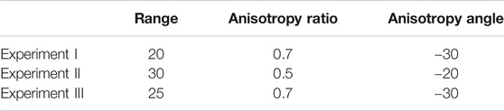
TABLE 3. Specific characterizations of variograms of the prior distribution, the unit for range is grid cells.

5.1 Experiment I

This experiment is conducted on Reservoir Model I with five levels corresponding to 82, 124, 310, 1,060, and 4,096 grid cells, respectively. A summary of the resource allocation for the different runs carried out in this experiment can be found in Table 4. The observation data for this experiment are generated based on seismic vintages at 4,000 and 8,000 days after production starts.

TABLE 4

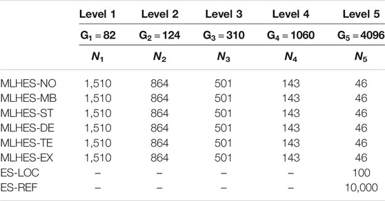
TABLE 4. Summary of resource allocation for the algorithms in Experiment I.

5.2 Experiment II

This experiment is conducted on Reservoir Model II. In this experiment, the presence of the oblique fault in the field interferes with coarsening the model. One way to handle this issue would be to avoid coarsening the grid around the fault area; however, this would reduce the computational advantage of the multilevel scheme. In order to keep the grid coarsening as it is, the fault is approximated with bigger “zigzags,” as depicted in Figure 6, for one realization of the logarithmic permeability field at different levels of coarseness. This makes the experiment to be more challenging than Experiment I, since in addition to coarsening the grid and upscaling the parameters, a structural characterization of the field (the fault) is also approximated.

MLHES is run with four levels corresponding to 124, 310, 1,060 and 4,096 grid cells, respectively. A summary of the resource allocation for the different algorithms carried out in this experiment can be found in Table 5. The observation data are generated based on seismic vintages at 5,000 and 10,000 days after beginning of production.

TABLE 5

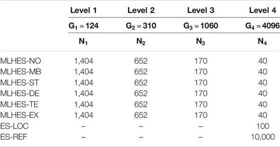
TABLE 5. Summary of resource allocation for the algorithms in Experiment II.

5.3 Experiment III

This experiment is conducted on Reservoir Model III. The coarsening of the grid is performed uniformly, so that also the regions near the wells are coarsened. Hence, a different type of MLME is generated. The number of grid cells is now complete powers of 2. Forming four levels of coarseness, the number of grid cells are 64, 256, 1,024, and 4,096. A summary of the resource allocation for the different algorithms carried out in this experiment can be found in Table 6. The observation data are generated based on seismic vintages at 4,000 and 8,000 days after production starts.

TABLE 6

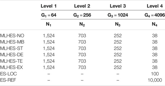
TABLE 6. Summary of resource allocation for the algorithms in Experiment III.

6 Numerical Results

The numerical results are assessed in two ways. First, we perform a quantitative analysis of the MLME-corrected model forecasts. Second, we perform a qualitative analysis of the results obtained when using the MLME-corrected forecasts in MLDA.

As for a quantitative analysis of success of MLME correction schemes, the normalized correction ratio for model forecasts at level l, $NC{R}_l$, defined as

$NC{R}_l\left(Z\right)=\left|\left(Y_l-U_L^l{Y}_L\right)\mathrm{\oslash }\left({\widehat{Y}}_l-U_L^l{Y}_L\right)\right|=\left|\left({\epsilon }_{l,\times }-{\zeta }_l\right)\mathrm{\oslash }{\zeta }_l\right|,(32)$

is considered. Here, $\mathrm{\oslash }$ is the Hadamard division and $\left|\text{*}\right|$ is the element-wise absolute value operator. If the correction scheme does not do any correction on a single element of NCR_l, it would result in that element to be equal to unity. Reduction in the error would result in the element moving toward zero, and an increase in the error would move that element toward infinity; hence, NCR_l is an indicator of the success of MLME correction schemes.

NCR_l is different for different realizations. In order to assess the success of each of the correction schemes jointly for all realizations, the sample median of each of the elements of NCR_l is computed. The median is chosen since the mean of NCR_l is not a good indicator of success (NCR_l has a lower bound at zero but has no upper bound, and outliers would affect it disproportionately). Then, the mean of the elements of the sample median of NCR_l are reported for different levels in all MLME correction schemes for the three experiments.

As for the qualitative assessment of the DA results, the mean and the variance of the posterior unknown parameters are compared between different algorithms. We have not considered any specific formulation for computation of the final multilevel statistics. Accordingly, the simplest formulation is chosen, that is, reuniting all the sub-ensembles and treating them as one ensemble for computation of a posteriori mean and variance fields. ES-LOC was tested with several ranges for localization (critical distances), and the best results are presented for each of the experiments.

6.1 Results of Experiment I

As can be seen in Table 7, $NC{R}_l$ is smaller in coarser models for all correction schemes. For a class of problems (including the problem considered here) where the model forecast can be seen as a spatially integrated response to a spatially varying parameter field, there exists a correlation between small-scale oscillations in the parameter domain and the nonlinearity strength of the mapping from parameter field to model forecast (see, e.g., [24, 25]). This correlation is such that coarsening the simulation grid and upscaling the associated parameters will generally result in weaker nonlinearity in the coarser forward models than the finer ones. The comparatively lower $NC{R}_l$ in coarser levels than finer ones can be due to this decrease in nonlinearity by a decrease in l and also due to omission of local fluctuations in coarser model forecasts. In the case of the telescopic scheme, this can also be attributed to an increase in the ensemble size, which reduces the Monte Carlo errors associated with estimation of the MLME errors. All the schemes, except for mean bias correction, are, on average, successful in reduction of MLME. Telescopic correction for level 4 (level $L-1$ in general) reduces to deterministic correction, but in coarser levels, it has performed better than deterministic correction, which, in turn, performs slightly better than stochastic correction.

TABLE 7

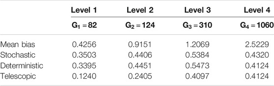
TABLE 7. Experiment I: Mean of the elements of the median vector of $NC{R}_l$ for different correction schemes.

Visual analysis of the mean permeability fields, given in Figure 7, shows that all MLHES variants are reasonably similar and more similar to ES-REF than ES-LOC is. This can be further confirmed by comparison of the variance fields given in Figure 8. The ES-LOC results presented here are based on the localization range of 40 grid cells. Additionally, no superiority of some MLME correction schemes over others is evident in visual assessment of the posterior mean and variance fields. The results from all MLHES variants are reasonably similar to the MLHES-EX results.

FIGURE 7

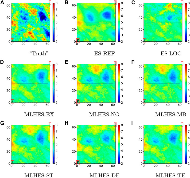
FIGURE 7. Experiment I: Mean of posterior logarithmic permeability field.

FIGURE 8

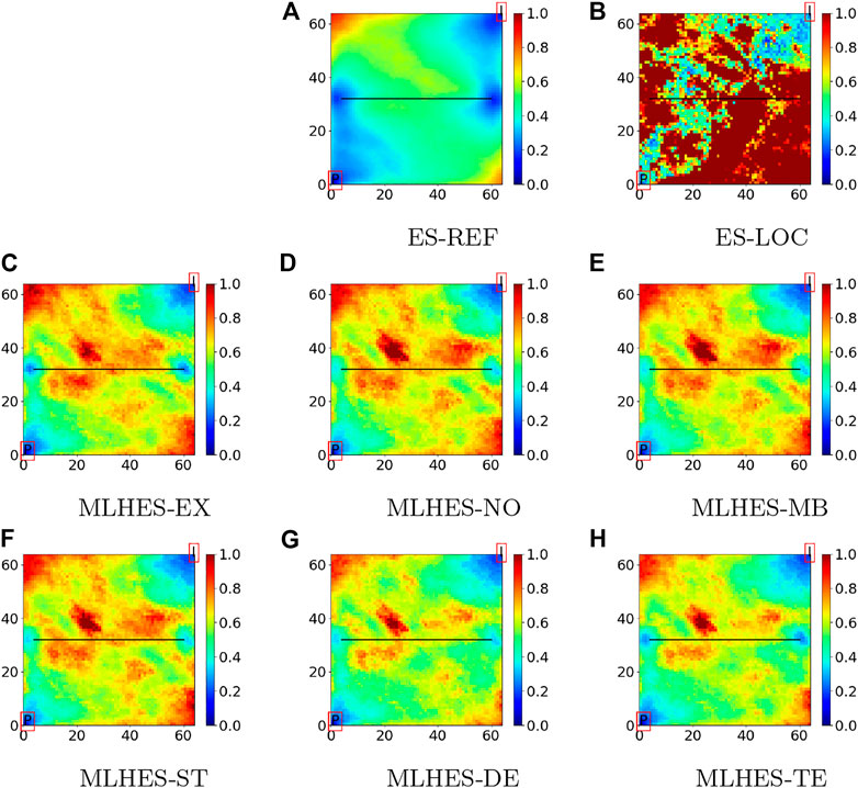
FIGURE 8. Experiment I: Variance of posterior logarithmic permeability field.

6.2 Results of Experiment II

Based on the trends in $NC{R}_l$, as can be seen in Table 8, the performance of the correction schemes has the same rank order as those of Experiment I, with telescopic correction showing the best performance, followed by deterministic, stochastic, and mean bias corrections. Visual analysis of the mean permeability fields, given in Figure 9, shows that all MLHES variants are reasonably similar and more similar to ES-REF than ES-LOC is. This can be further confirmed by comparison of the variance fields given in Figure 10. The ES-LOC results presented here are based on the localization range of 50 grid cells. Additionally, no superiority of some MLME correction schemes over others is evident in visual assessment of the posterior mean and variance fields. The results from all MLHES variants are reasonably similar to the MLHES-EX results.

TABLE 8

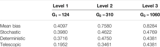
TABLE 8. Experiment II: Mean of the elements of the median vector of $NC{R}_l$ for different correction schemes.

FIGURE 9

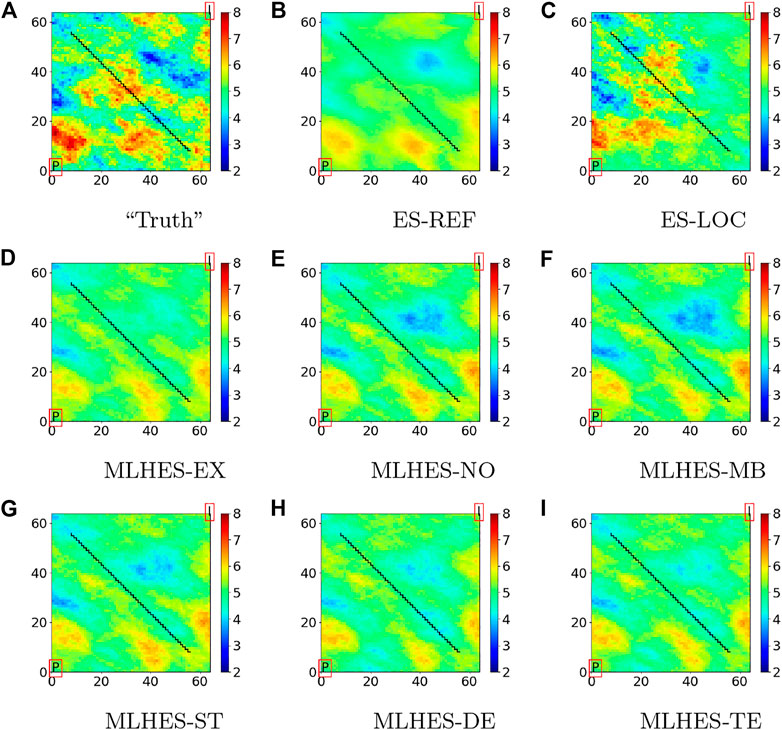
FIGURE 9. Experiment II: Mean of posterior logarithmic permeability field.

FIGURE 10

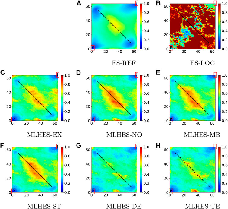
FIGURE 10. Experiment II: Variance of posterior logarithmic permeability field.

6.3 Results of Experiment III

From Table 9, it is seen that $NC{R}_l$ is comparatively higher in this experiment than the previous two experiments. The rank order of the performances stays the same, but the quality of correction has deteriorated for all the MLME correction schemes, except for the mean bias correction which has slightly improved.

TABLE 9

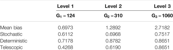
TABLE 9. Experiment III: Mean of the elements of the median vector of $NC{R}_l$ for different correction schemes.

Visual analysis of the mean permeability fields, given in Figure 11, shows that all MLHES variants are reasonably similar and more similar to ES-REF than ES-LOC. This can be further confirmed by comparison of the variance fields given in Figure 12. The ES-LOC results presented here are based on the localization range of 40 grid cells. Additionally, no superiority of some MLME correction schemes over others is evident in visual assessment of the posterior mean and variance fields. The results from all MLHES variants are reasonably similar to the MLHES-EX results.

FIGURE 11

FIGURE 11. Experiment III: Mean of posterior logarithmic permeability field.

FIGURE 12

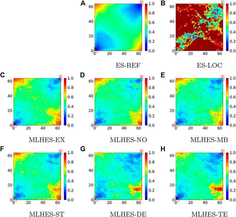
FIGURE 12. Experiment III: Variance of posterior logarithmic permeability field.

7 Summary and Conclusion

With large amounts of simultaneous data, like inverted seismic data in reservoir modeling, negative effects of Monte Carlo errors in straightforward ensemble-based data assimilation (DA) are enhanced, typically resulting in underestimation of parameter uncertainties. Multilevel simulations utilize a selection of models for the same entity that constitute hierarchies both in fidelities and computational costs. Multilevel data assimilation (MLDA) utilizes multilevel simulations in the forecast step. MLDA therefore renders the possibility of decreasing Monte Carlo errors without increasing the total computational cost, but MLDA will also introduce multilevel modeling errors (MLME) that are not present in conventional simulation results. The underlying assumption is therefore that the gain in reducing the Monte Carlo error is larger than the loss in introducing the MLME. If the MLME could be approximately accounted for, however MLDA performance could be further improved.

We have estimated and approximately accounted for the MLME. Four computationally inexpensive approximate MLME correction schemes have been considered. We have denoted these schemes mean bias correction, stochastic correction, deterministic correction, and telescopic correction. The three latter schemes have been developed in this work. The abilities of the four schemes to correct for the MLME have been assessed in two ways, utilizing numerical experiments with three selected reservoir models.

First, statistics for the normalized correction ratios for model forecasts at each level were compared. The results showed that the correction schemes were capable of reducing the MLME, but the amount of reduction depended on the case and on the level. In general, the MLME correction schemes were more successful in correcting the MLME in the coarser levels than the finer ones, with telescopic correction showing the best performance followed by deterministic correction, stochastic correction, and mean bias correction.

Second, we assessed the performances of the different MLME-corrected model forecasts in assimilation of inverted seismic data, using the multilevel hybrid ensemble smoother (MLHES). The resulting posterior mean and variance fields with and without MLME correction were visually compared to results obtained from conventional ensemble smoother (ES) with localization, utilizing results obtained with conventional ES with an unrealistically large ensemble size as the gold standard. It was found that MLHES with and without MLME correction outperformed conventional ES with localization.

The use of all four MLME correction schemes, and in fact also MLDA without MLME correction, mostly resulted in posterior parameter estimates with similar quality. For each example, we also ran a computationally much more costly MLDA variant where the MLME had been exactly accounted for in the model forecasts (termed MLHES-EX in Sections 5–6). No differences in quality between results obtained with MLHES-EX and results obtained with several of the computationally inexpensive MLDA variants were found in all three examples. We have run several examples in addition to those presented in the article. In none of these examples did the computationally inexpensive MLDA variants produce poor results, and straightforward MLHES (i.e., without any MLME correction) produced results of similar quality. Altogether, these results indicate that the MLHES is reasonably robust toward MLMEs.

Further investigation concerning the robustness of MLHES with and without MLME correction can be conducted for additional reservoir models with different types of MLMEs than those considered here. On the other hand, the MLME correction techniques can be further developed. Their current versions address the MLME of spatially distributed data on their associated grid cells independently, that is, spatial correlations of the MLME are not considered. It would be interesting to consider spatial correlation of the MLME in future work.

Data Availability Statement

The raw data supporting the conclusions of this article will be made available by the authors, without undue reservation.

Author Contributions

MN is a Ph.D. student, and TB, KF, and TM are supervising him in his research. Accordingly, MN did the details of the research and most of writing with the help of his supervisors.

Conflict of Interest

The authors declare that the research was conducted in the absence of any commercial or financial relationships that could be construed as a potential conflict of interest.

Acknowledgments

The authors acknowledge financial support from the NORCE research project “Assimilating 4D Seismic Data: Big Data Into Big Models” which is funded by industry partners, Aker BP ASA, Equinor Energy AS, Lundin Energy Norway AS, Repsol Norge AS, Shell Global Solutions International B.V., Total E&P Norge AS, and Wintershall Dea Norge AS, as well as the Research Council of Norway (PETROMAKS2). We also thank Schlumberger for providing academic software licenses to ECLIPSE.

Footnotes

¹Nezhadali, M., Bhakta, T., Fossum, K., and Mannseth, T. Iterative multilevel assimilation of inverted seismic data. Submitted

References

1. Chen, Y, and Oliver, DS. Ensemble Randomized Maximum Likelihood Method as an Iterative Ensemble Smoother. Math Geosci (2012). 44(1):1–26. doi:10.1007/s11004-011-9376-z

CrossRef Full Text | Google Scholar

2. Emerick, AA, and Reynolds, AC. Ensemble Smoother with Multiple Data Assimilation. Comput Geosci (2013). 55:3–15. doi:10.1016/j.cageo.2012.03.011

CrossRef Full Text | Google Scholar

3. Luo, X, Bhakta, T, and Nævdal, G. Correlation-based Adaptive Localization with Applications to Ensemble-Based 4d-Seismic History Matching. SPE J (2018). 23(02):396–427. doi:10.2118/185936-pa

CrossRef Full Text | Google Scholar

4. Lorentzen, RJ, Bhakta, T, Grana, D, Luo, X, Valestrand, R, and Nævdal, G. Simultaneous Assimilation of Production and Seismic Data: Application to the Norne Field. Comput Geosci (2019). 12:1–14. doi:10.1007/s10596-019-09900-0

CrossRef Full Text | Google Scholar

5. Gaspari, G, and Cohn, SE. Construction of Correlation Functions in Two and Three Dimensions. Q.J R Met. Soc. (1999). 125(554):723–57. doi:10.1002/qj.49712555417

CrossRef Full Text | Google Scholar

6. Chen, Y, and Oliver, DS. Cross-covariances and Localization for Enkf in Multiphase Flow Data Assimilation. Comput Geosci (2010). 14(4):579–601. doi:10.1007/s10596-009-9174-6

CrossRef Full Text | Google Scholar

7. Emerick, A, and Reynolds, A. Combining Sensitivities and Prior Information for Covariance Localization in the Ensemble Kalman Filter for Petroleum Reservoir Applications. Comput Geosci (2011). 15(2):251–69. doi:10.1007/s10596-010-9198-y

CrossRef Full Text | Google Scholar

8. He, J, Sarma, P, and Durlofsky, LJ. Reduced-order Flow Modeling and Geological Parameterization for Ensemble-Based Data Assimilation. Comput Geosciences (2013). 55:54–69. doi:10.1016/j.cageo.2012.03.027

CrossRef Full Text | Google Scholar

9. Tarrahi, M, Elahi, SH, and Jafarpour, B. Fast Linearized Forecasts for Subsurface Flow Data Assimilation with Ensemble Kalman Filter. Comput Geosci (2016). 20(5):929–52. doi:10.1007/s10596-016-9570-7

CrossRef Full Text | Google Scholar

10. Fossum, K, and Mannseth, T. Coarse-scale Data Assimilation as a Generic Alternative to Localization. Comput Geosci (2017). 21(1):167–86. doi:10.1007/s10596-016-9602-3

CrossRef Full Text | Google Scholar

11. Hatfield, S, Subramanian, A, Palmer, T, and Düben, P. Improving Weather Forecast Skill through Reduced-Precision Data Assimilation. Monthly Weather Rev (2018). 146(1):49–62. doi:10.1175/mwr-d-17-0132.1

CrossRef Full Text | Google Scholar

12. Fossum, K, Mannseth, T, and Stordal, AS. Assessment of Multilevel Ensemble-Based Data Assimilation for Reservoir History Matching. Comput Geosci (2020). 24(1):217–39. doi:10.1007/s10596-019-09911-x

CrossRef Full Text | Google Scholar

13. Hoel, H, Law, KJH, and Tempone, R. Multilevel Ensemble Kalman Filtering. SIAM J Numer Anal (2016). 54(3):1813–39. doi:10.1137/15m100955x

CrossRef Full Text | Google Scholar

14. de Moraes, RJ, Hajibeygi, H, and Jansen, JD. A Multiscale Method for Data Assimilation. Comput Geosciences (2019). 12:1–18. doi:10.5194/egusphere-egu21-3880

CrossRef Full Text | Google Scholar

15. Fossum, K, and Mannseth, T. “A Novel Multilevel Method for Assimilating Spatially Dense Data,” in ECMOR XVI-16th European Conference on the Mathematics of Oil Recovery, Vol. 2018. London: European Association of Geoscientists & Engineers (2018). 1–12.

Google Scholar

16. Nezhadali, M, Bhakta, T, Fossum, K, and Mannseth, T. “A Novel Approach to Multilevel Data Assimilation,” in ECMOR XVII, Vol. 2020. London: European Association of Geoscientists & Engineers (2020). 1–13.

Google Scholar

17. Evensen, G. Accounting for Model Errors in Iterative Ensemble Smoothers. Comput Geosci (2019). 23(4):761–75. doi:10.1007/s10596-019-9819-z

CrossRef Full Text | Google Scholar

18. Kaipio, J, and Somersalo, E. Statistical Inverse Problems: Discretization, Model Reduction and Inverse Crimes. J Comput Appl Math (2007). 198(2):493–504. doi:10.1016/j.cam.2005.09.027

CrossRef Full Text | Google Scholar

19. Schlumberger, L. Eclipse Reservoir Simulation Software V2016 (2016). Technical Description Manual.

20. Batzle, M, and Wang, Z. Seismic Properties of Pore Fluids. Geophys. (1992). 57(11):1396–408. doi:10.1190/1.1443207

CrossRef Full Text | Google Scholar

21. Fahimuddin, A. 4D Seismic History Matching Using the Ensemble Kalman Filter (EnKF): Possibilities and challenges. Ph.D. Thesis. The University of Bergen (2010). doi:10.2118/131453-ms

CrossRef Full Text

22. Axelsson, O. Iterative Solution Methods. Cambridge: Cambridge University Press (1996).

23. Furrer, R, and Bengtsson, T. Estimation of High-Dimensional Prior and Posterior Covariance Matrices in Kalman Filter Variants. J Multivar. Anal (2007). 98(2):227–55. doi:10.1016/j.jmva.2006.08.003

CrossRef Full Text | Google Scholar

24. Chavent, C, and Liu, J. Multiscale Parametrization for the Estimation of a Diffusion Coefficient in Elliptic and Parabolic Problems. IFAC Proc Vol. (1989). 22(4):193–202. doi:10.1016/s1474-6670(17)53542-9

CrossRef Full Text | Google Scholar

25. Grimstad, A-A, and Mannseth, T. Nonlinearity, Scale, and Sensitivity for Parameter Estimation Problems. SIAM J Sci Comput (2000). 21(6):2096–113. doi:10.1137/s1064827598339104

CrossRef Full Text | Google Scholar

Appendix A: MLHES pseudo-code

Algorithm 1: MLHES Algorithm