Coherence Resonance in Random Erdös-Rényi Neural Networks: Mean-Field Theory

1 Introduction

Synchronization is a well characterized phenomenon in natural systems [1]. A confluence of experimental studies indicate that synchronization may be a hallmark pattern of self-organization [2–4]. While various mechanisms are possible, synchronization may emerge notably through an enhancement of internal interactions or via changes in external stimuli statistics. A specific type of synchronization can occur due to random external perturbations, leading to a noise-induced coherent activity. Such a phenomenon is called coherence resonance (CR) and has been found experimentally in solid states [5], nanotubes [6] and in neural systems [7, 8]. Theoretical descriptions of CR have been developed for single excitable elements [9, 9, 10], for excitable populations [11] and for clustered networks [12].

In general, stimulus-induced synchronization is well-known in neural systems [2]. Synchronization has been observed intracranially in the presence of noise between single neurons in specific brain areas [13, 14] and between brain areas [15–17]. The source of these random perturbations is still under debate. In this context, it is interesting to mention that [18] have found that the ascending reticular arousal system (ARAS) affects synchronization in the visual cortex. The ARAS provides dynamic inputs to many brain areas [19–21]. It has thus been hypothesized that synchronization in the visual system represents a CR effect triggered by ARAS-mediated drive. This hypothesis has been supported recently by [22] showing in numerical simulations that an intermediate intensity of noise maximizes the interaction in a neural network of Hodgkin-Huxley neurons. Furthermore, recent theoretical work [21] has provided key insights on how human occipital electrocorticographic γ-activity (40–120 Hz) commonly observed with open eyes [21] is closely linked to CR. Coherence resonance has further been associated with states of elevated information processing and transfer [22], which are difficult to assess in the absence of mean-field descriptions. For illustration, Figure 1 (upper panel) shows average network activity for increasing noise intensities $D_1$ and one observes a jump from non-oscillatory to oscillatory activity. Moreover, the figure presents very low coherence in the network under study for weak and strong noise intensities $D_1$, whereas high coherence emerges for intermediate noise intensities (bottom panel). In the present work, we will explain this noise-induced coherence by a mean-field description.

FIGURE 1

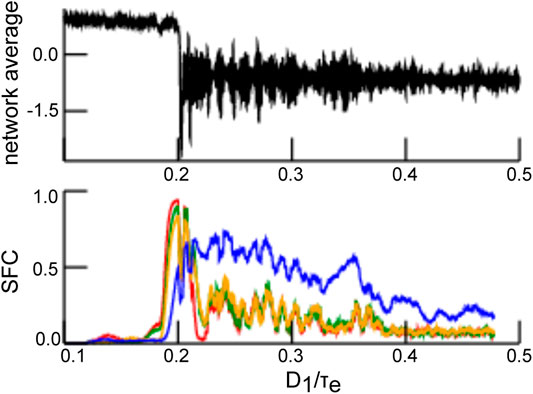
FIGURE 1. Synchronization dependent on noise intensity as a marker of coherence resonance. The top panel shows the network average of $\mathit{V}$ in Eq. 1 and the bottom panel provides the Spike Field Coherence (SFC) in the $\text{Θ}-$ (red), $\alpha -$ (green), $\beta -$ (orange) and $\gamma -$ (blue) frequency range. For low noise intensity $D_1/{\tau }_e$ there is no SFC, intermediate noise intensity yields strong SFC while large noise intensities diminish SFC again. To gain the SFC values, we have integrated in time the model system with ${10}^4$ time steps while increasing the noise variance according to (Eq. 7). For illustration reasons, the SFC-values have been averaged by a sliding window of length $\text{Δ}\left(D_1/{\tau }_e\right)=0.004$. Definitions are given in section 2 and parameters are the same as in Figure 4 with $q=1$.

To better understand the mechanisms underlying CR and its impact on information processing, we consider a simple two-population Erdös-Rényi network of interconnected McCullogh-Pitts neurons. Our goal is to use this model to provide some insight into the emergence of stimulus-induced synchronization in neural systems and its influence on the neural network’s information content. The neural network under study has random connections, a simplification inspired from the lack structure neural circuits possess at microscopic scales. Previous studies [23] have shown that such systems are capable of noise-induced CR. Building on these results, we here provide a rigorous derivation of a mean-field equation based on an appropriate eigenmode decomposition to highlight the role of the network’s connectivity–Erdös-Rényi more specifically eigenspectrum in supporting accurate mean-field representations. We extend previous results by further considering both global (all neurons are stimulated) and partial (some neurons are stimulated) stochastic stimulation and its impact on CR similar to some previous studies [24–26]. This partial stimulation is both more general and realistic than global stimulation as considered in most previous studies [11, 23, 27]. We apply our results to both zero-mean Gaussian and Poisson-like stochastic stimuli, and derive the resulting mean-field description. It is demonstrated rigorously that partial stochastic stimulation shifts the system’s dynamic topology and promotes CR, compared to global stimulation. We confirm and explore the presence of CR using various statistical measures.

2 Materials and Methods

We first introduce the network model under study, motivate the mean-field description, mentions the nonlinear analysis employed and provides details on the statistical evaluation.

2.1 The Network Model

Generically, biological neuronal networks are composed of randomly connected excitatory and inhibitory neurons, which interact through synapses with opposite influence on post-synaptic cells. We assume neural populations of excitatory $\mathrm{ℰ}$ and inhibitory $\mathrm{ℐ}$ neurons with N neurons in each population. Excitatory neurons in $\mathrm{ℰ}$ excite each other through the connectivity matrix $\mathit{F}$, and excite inhibitory neurons in $\mathrm{ℐ}$ through the connectivity matrix $\mathit{M}$. Similarly, neurons in $\mathrm{ℐ}$ inhibit each other by $\mathit{F}$ and inhibit excitatory neurons through the connectivity matrix $\mathit{M}$. Hence, $\mathit{F}$ and $\mathit{M}$ represent the intra-population and inter-population synaptic connections, respectively. Mathematically, such neural population interactions are described by a $2N$ dimensional non-linear dynamical system governing the evolution of the state variable vectors $\mathbf{V},\mathbf{W}\in {\mathrm{ℝ}}^N$,

$\begin{array}{cc}{\tau }_e\frac{d\mathbf{V}}{dt}& =-\mathbf{V}+\mathbf{F}{\mathbf{S}}_1\left[\mathbf{V}\right]-\mathbf{M}{\mathbf{S}}_2\left[\mathbf{W}\right]+\mathit{e}{I}^e+{\mathit{\xi }}^e\left(t\right)\\ {\tau }_i\frac{d\mathbf{W}}{dt}& =-\mathbf{W}+\mathbf{M}{\mathbf{S}}_1\left[\mathbf{V}\right]-\mathbf{F}{\mathbf{S}}_2\left[\mathbf{W}\right]+\mathit{e}{I}^i+{\mathit{\xi }}^i\left(t\right).\end{array}(1)$

This formulation is reminiscent of many rate-based models discussed previously [28], where it is assumed that neuronal activity is asynchronous and synaptic response functions are of first order. The state variables $\mathbf{V}$ and $\mathbf{W}$ represent excitatory and inhibitory dendritic currents, respectively. The terms ${\mathit{\xi }}^{e,i}$ represent respective stochastic inputs from various sources, such as ion channel fluctuations, stochastic input from other brain areas or external stimuli not directly accounted for in the model [29]. More specifically, we assume noise ${\mathit{\xi }}^{e,i}\in {\mathrm{ℝ}}^N$, constant input $I^{e,i}$ with $\mathit{e}={\left(1,\dots ,1\right)}^t$. The connectivity matrices are defined by $\mathbf{F},\mathbf{M}\in {\mathrm{ℝ}}^{N\times N}$ while the nonlinear transfer function is given by ${\mathbf{S}}_{\mathrm{1,2}}\left[\mathrm{u}\right]\in {\mathrm{ℝ}}^N$ with ${\left({\mathbf{S}}_1\left[\mathbf{u}\right]\right)}_n=H_{0}S\left(u_n\right)$, ${\left({\mathbf{S}}_2\left[\mathbf{u}\right]\right)}_n=S\left(u_n\right)$, $H_0>0$ and the scalar transfer function $S\left(u\right)>0\forall u\in \mathrm{ℝ}$. Specifically, we will consider the transfer function $S\left(u\right)=\text{Θ}\left(u\right)$ with the Heaviside function $\text{Θ}\left(u\right)=0\forall u<0,\text{Θ}\left(u\right)=1\forall u\ge 0$. In addition, the synaptic time scales are ${\tau }_{e,i}$.

The present work considers directed Erdös-Rényi networks (ERN) with connection probability density $c=0.95$, i.e. both neuron populations exhibit intra-population and inter-population non-sparse random connections. Let us assume $\mathbf{F}=\mathbf{A}{\mathit{F}}_0$, $\mathrm{M}=\mathbf{A}{M}_0$ and $\mathbf{A}$ is the non-symmetric adjacency matrix of the ERN for which ${\left(\mathit{A}\right)}_{nm}=0$ with probability $1-c$ and ${\left(\mathit{A}\right)}_{nm}=1/cN$ with probability c. At first, let $\mathit{A}=\mathit{S}+\mathit{U}$ with the symmetric matrix $\mathit{S}=\left(\mathit{A}+{\mathit{A}}^t\right)/2$, the antisymmetric matrix $\mathit{U}=\left(\mathit{A}-{\mathit{A}}^t\right)/2$ and the eigenvalues ${\lambda }_A$ and ${\lambda }_S$ of the matrix $\mathit{A}$ and $\mathit{S}$, respectively. Then $\mathrm{ℛ}e\left({\lambda }_A\right)={\lambda }_S$, i.e. the real part of the eigenvalue spectrum in the directed (i.e. non-symmetric) and non-directed (i.e. symmetric) random matrix $\mathit{A}$ and $\mathit{S}$ is identical. Moreover, for non-directed ERNs with symmetric adjacency matrix and $N\to \infty$ its edge spectrum contains the maximum eigenvalue ${\lambda }_1=1$ with eigenvector ${\mathit{v}}_1={\left(\mathrm{1,1},\dots ,1\right)}^t$ [30–33] and the bulk spectrum has the maximum eigenvalue

$\begin{array}{l}{\lambda }_2=\frac{2\sigma \sqrt{N}}{cN}\\ =\frac{2\sqrt{1-c}}{\sqrt{cN}},\end{array}(2)$

with the corresponding Bernoulli distribution variance ${\sigma }^2=c\left(1-c\right)$. It is obvious that ${\lambda }_2\ll {\lambda }_1$ and ${\lambda }_2\approx 0$ for large mean degree $cN$. Since $\mathrm{ℛ}e\left({\lambda }_A\right)={\lambda }_S$, the finite-size non-symmetric connectivity matrix $\mathit{F}$ ($\mathit{M}$) has a maximum eigenvalue ${\lambda }_1\approx F_0$ and ${\lambda }_{n>1}\approx 0$ (${\lambda }_1\approx {\mathit{M}}_0,$${\lambda }_{n>1}\approx 0$). If c decreases, then ${\lambda }_2$ increases, i.e. the spectral gap decreases, and this approximation does not hold anymore. The Supplementary Appendix illustrates the limits of this approximation in numerical simulations. Figure 2A shows the single maximum eigenvalue ${\lambda }_1$ of $\mathit{A}$ representing the edge spectrum and the other very small eigenvalues of the bulk spectrum. Hence, the matrix $\mathit{F}$ has maximum eigenvalue $F_0$ and the other eigenvalues vanish. The same holds for matrix $\mathit{M}=M_0\mathit{A}$ with a maximum eigenvalue $M_0$. Figure 2B shows the real and imaginary part of the eigenvectors. The eigenvectors of the bulk spectrum $\left(i>1\right)$ have uniformly distributed elements in good accordance with theory of symmetric ER networks [34]. The eigenvector of the edge spectrum is ${\mathbf{\Phi }}_1={\left(1,\dots ,1\right)}^t$, see Figure 2C.

FIGURE 2

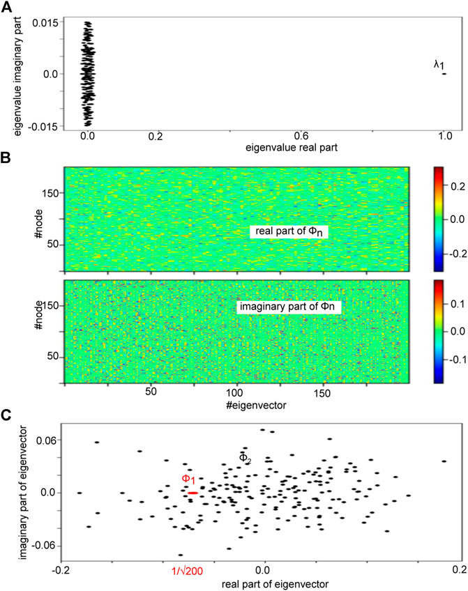
FIGURE 2. Eigenvalue spectrum of an Erdös-Rényi adjency matrix A under study and its eigenbasis. (A) The plot shows the eigenvalues in the complex plane demonstrating a clear spectral gap between the first eigenvalue ${\lambda }_1$ and the other eigenvalues ${\lambda }_{n>1}$. (B) The panels show the real (top) and imaginary (bottom) part of all unit-normalized eigenvectors for illustration. They appear to be random reflecting the random network topology. (C) The normalized eigenvector ${\mathbf{\Phi }}_1\approx \left(1,\dots ,1\right)/\sqrt{N}$ with maximum eigenvalue ${\lambda }_1\approx 1$ plotted in complex plane together with the eigenvector ${\mathbf{\Phi }}_2$ of the second largest eigenvalue ${\lambda }_2=0.015+i0.0006$. Each dot corresponds to a complex-numbered vector entry in the complex plane. This result confirms the choice ${\mathbf{\Phi }}_1\approx \left(1,\dots ,1\right)$ in Eq. 9.

Moreover, we assume that each noise process at inhibitory neurons ${\left({\mathit{\eta }}^i\right)}_n={\eta }_n^i$ at network node n is Gaussian distributed with zero mean, noise intensity $D_2$ and uncorrelated in time

$\langle {\xi }_n^i\left(t\right){\xi }_m^i\left(\tau \right)\rangle =2D_2{\delta }_{nm}\delta \left(t-\tau \right),$

Conversely each noise process at excitatory neurons ${\xi }_n^e$ belongs to a certain class ${\mathcal{G}}_m,m=1,\dots ,M$ of M classes [23]. Noise processes in a specific class ${\mathcal{G}}_m$, i.e. $n\in {\mathcal{G}}_m$, share their mean ${\overline{\xi }}_m^e$ and variances $D_1^m$, i.e.

$\langle {\xi }_k^e\left(t\right){\xi }_l^i\left(\tau \right)\rangle =2D_1^m{\delta }_{kl}\delta \left(t-\tau \right),k,l\in {\mathcal{G}}_m,$

In the following, we assume two classes $M=2$ with ${\overline{\xi }}_1^e\ne 0,D_1^1=D_1$ and ${\overline{\xi }}_2^e=0,D_1^2=0$, i.e. only a subset of nodes $n\in {\mathcal{G}}_1$ are stimulated. Hence we consider a partial stimulation at number of nodes $N_1=\left|{\mathcal{G}}_1\right|$.

In biological neural systems, the input to a neural population is well-described by incoming spike trains that induce dendritic currents at synaptic receptors. According to renewal theory, neurons emit spike trains whose interspike interval obeys a Poisson distribution [35]. Then incoming spike trains at mean spike rate r induce random responses at excitatory synapses with time constant ${\tau }_{\text{in}}$. This random process $I_{\text{in}}\left(t\right)$ has the ensemble mean $\text{E}\left[I_{\text{in}}\right]=w_{\text{in}}r{\tau }_{\text{in}}$ and ensemble variance $\text{Var}\left[I_{\text{in}}\right]=w_{\text{in}}^{2}r{\tau }_{\text{in}}/2$ [36] assuming the synaptic coupling weight $w_{\text{in}}$. Since a Poisson distribution converges to a Gaussian distribution for large enough mean, we implement this input current as a Gaussian random process with mean $\text{E}\left[I_{\text{in}}\right]$ and variance $\text{Var}\left[I_{\text{in}}\right]$ while ensuring the validity of this approximation by a large enough input firing rate ${\lambda }_{in}$. It is important to point out that for Poisson noise, in contrast to the zero-mean Gaussian noise, both mean and variance are proportional to the input firing rate.

2.2 Conventional Mean-Field Analysis

To compare mesoscopic neural population dynamics to macroscopic experimental findings, it is commonplace to describe the network activity by the mean population response, i.e. the mean-field dynamics [37–39]. A naive mean-field approach was performed in early neuroscience studies [40–42], in which one blindly computes the mean network activity to obtain

$\begin{array}{cc}{\tau }_e\frac{dE\left[V\right]}{dt}& =-E\left[V\right]+\mathbf{f}{\mathbf{S}}_1\left[\mathbf{V}\right]-\mathbf{m}{\mathbf{S}}_2\left[\mathbf{W}\right]+\mathit{e}{I}^e\\ {\tau }_i\frac{dE\left[W\right]}{dt}& =-E\left[W\right]+\mathbf{m}{\mathbf{S}}_1\left[\mathbf{V}\right]-\mathbf{f}{\mathbf{S}}_2\left[\mathbf{W}\right]+\mathit{e}{I}^i,\end{array}(3)$

with the network average $E\left[x\right]={\displaystyle {\sum }_k}{x}_k/N$ and ${\left(\mathit{f}\right)}_k={\displaystyle {\sum }_l}{\mathit{F}}_{lk}/N,{\left(\mathit{m}\right)}_k={\displaystyle {\sum }_l}{\mathit{M}}_{lk}/N$ assuming zero-mean external noise with ${\displaystyle {\sum }_k{\left({\mathit{\xi }}^{e,i}\right)}_k}=0$. In addition, one may assume identical network interactions with ${\left(\mathit{f}\right)}_k={\mathit{f}}_0/N=\text{const}$, ${\left(\mathit{m}\right)}_k=m_0/N=\text{const}$ and the simplifying but questionable linear assumption.

$E\left[S_{\mathrm{1,2}}\left(x\right)\right]=S_{\mathrm{1,2}}\left(E\left[x\right]\right).(4)$

Combined, these assumptions lead to mean-field equations.

$\begin{array}{c}{\tau }_e\frac{dE\left[V\right]}{dt}=-E\left[V\right]+f_0{S}_1\left[E\left[V\right]\right]-m_0{S}_2\left[E\left[W\right]\right]\\ +\mathit{e}{I}^e\\ {\tau }_i\frac{dE\left[W\right]}{dt}=-E\left[W\right]+m_0{S}_1\left[E\left[V\right]\right]-f_0{S}_2\left[E\left[W\right]\right].\\ +\mathit{e}{I}^i\end{array}(5)$

In this approximate description, additive noise does not affect the system dynamics. The assumption (Eq. 4) is very strong and typically not valid. In a more reasonable ansatz.

$\begin{array}{c}E\left[S_{\mathrm{1,2}}\left(x\right)\right]=E\left[S_{\mathrm{1,2}}\left(x_0\right)+{\displaystyle \sum }_{n=1}^{\infty }\frac{1}{n!}{S}_{\mathrm{1,2}}^{\left(n\right)}{\left(x-x_0\right)}^n\right]\\ =S_{\mathrm{1,2}}\left(x_0\right)+{\displaystyle \sum }_{n=1}^{\infty }\frac{1}{n!}{S}_{\mathrm{1,2}}^{\left(n\right)}E\left[{\left(x-x_0\right)}^n\right]\\ =\mathrm{ℱ}\left(E\left[x\right],E\left[x^2\right],E\left[x^3\right],\dots \right),\end{array}(6)$

with $S_{\mathrm{1,2}}^{\left(n\right)}=\partial S_{\mathrm{1,2}}^n\left(x\right)/\partial x^n$ computed at an arbitrary point $x=x_0$ and a function ${\mathrm{ℱ}}_{\mathrm{1,2}}\in \mathrm{ℝ}$. Hence the dynamics of the mean-field $E\left[V\right]$ depends on the higher-order statistical orders $E\left[V^n\right]$ via the nonlinear function $E\left[S_{\mathrm{1,2}}\left(V\right)\right]$. This is called the closure problem that is solvable in specific cases only [43].

Motivated by previous studies on stochastic bifurcations [44–53], in which additive noise may tune the stability close to the bifurcation point, the present work shows how additive noise strongly impacts the nonlinear dynamics of the system for arbitrary noise intensity and away from the bifurcation. Previous ad-hoc studies have already used mean-field approaches [23, 54, 55] which circumvents the closure problem (Eq. 6) through a different mean-field ansatz. These motivational studies left open a more rigorous derivation. This derivation will be given in the present work: presenting in more detail its power and its limits of validity.

2.3 Equilibria, Stability and Quasi-Cycles

The dynamic topology of a model differential equation system may be described partially by the number and characteristics of its equilibria. In general, for the non-autonomous differential equation system

$\dot{\mathit{z}}=\mathit{Az}+\mathit{N}\left(\mathit{z}\right)+\mathit{I}\left(t\right),$

with state variable $\mathit{z}\in {\mathrm{ℝ}}^N$, the driving force $\mathit{I}\in {\mathrm{ℝ}}^N$, the nonlinear vector $\mathit{N}\in {\mathrm{ℝ}}^N$ and the matrix $\mathit{A}\in {\mathrm{ℝ}}^{N\times N}$, it is insightful to consider the equilibria of the corresponding autonomous system ${\mathit{z}}_0$ with $\dot{\mathit{z}}=0$ yielding the implicit condition

$\mathit{A}{\mathit{z}}_0=-\mathit{N}\left({\mathit{z}}_0\right),$

The stability of an equilibrium ${\mathit{z}}_0$ is given by the eigenvalue spectrum of the corresponding Jacobian

$\mathit{J}=\mathit{A}+\nabla {\mathit{N}}^0,$

where ${\left(\nabla {\mathit{N}}^0\right)}_{ij}=\partial N_i\left(\mathit{z}\right)/\partial z_j$ computed at ${\mathit{z}}_0$. The eigenvalues $\left\{{\lambda }_k\right\}$ of $\mathit{J}$ can be written as ${\lambda }_k=a_k+i2\pi {\nu }_k$ with the damping $a_k$ and the eigenfrequency ${\nu }_k$. Asymptotically stable equilibria have $\mathrm{\Re }\left({\lambda }_k\right)<0$, e.g. stable foci have $a_k<0,{\nu }_k\in \mathrm{ℝ}$. Linear response theory tells that noise-driven linear systems, whose deterministic dynamics exhibit a stable focus, exhibit quasi-cycles with a spectral power peak close to the eigenfrequency, see e.g. [51, 56, 57]. The smaller the noise intensity, the closer is the spectral peak frequency to the eigenfrequency. Hence, the eigenfrequency ${\nu }_k$ provides a reasonable estimate of the quasi-cycle spectral peak.

2.4 Numerical Simulations

The Langevin Eq. 1 have been integrated over time utilizing the Euler-Maruyama scheme [58]. Table 1 presents the parameters used. In certain cases, the noise variance has been changed over time t according to

$D_1\left(t\right)=D_{\text{min}}+\frac{D_{\text{max}}-D_{\text{min}}}{T}t,(7)$

with the maximum integration time T and the maximum and minimum noise variance values $D_{\text{max}}$ and $D_{\text{min}}$, respectively.

TABLE 1

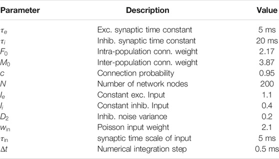
TABLE 1. Parameter set of model (1).

2.5 Numerical Spectral Data Analysis

Since prominent oscillations of the network mean activity indicates synchronized activity in the population, we have computed the power spectrum of the network mean activity $\begin{array}{l}\overline{V}\left(t\right)={\Sigma }_{n=1}^N\left(V_n\left(t\right)/N\right)\\ \end{array}$ employing the Bartlett-Welch method with overlap rate 0.8. To gain a power spectrum with frequency resolution $\text{Δ}f$, the Bartlett-Welch segments were chosen to the length $1/\text{Δ}f$ and the time series had a duration of 5 s for the zero-mean Gaussian noise and $8\text{s}$ for the Poisson noise stimulation.

In addition to the power spectrum, the synchronization between single neuron spike activity and the dendritic current reflects the degree of coherence in the system. To this end, we have computed the Spike Field Coherence (SFC) [59]. To estimate the SFC, we have chosen a time window of 5s for zero-mean Gaussian stimulation and 8s for Poisson stimulation and computed the spike-triggered average and power spectra in these time windows to compute the SFC for each frequency. Then we have averaged the SFC in the $\text{Θ}-$ (4–8 Hz), $\alpha -$ (8–12 Hz), $\beta -$ (12–20 Hz) and $\gamma -$ (25–60 Hz) frequency band to gain an average SFC in the corresponding band. This standard measure estimates the coherence between spikes, that occur if $H\left[V_n\right]\left(t\right)=1$, and their corresponding dendritic currents $V_n\left(t\right)$ at the same cell averaged over all cells in the excitatory population. Significant differences of SFC at different noise intensities are evaluated by an unpaired Welch t-test with $\alpha =0.05$.

2.6 Information Measures

Coherence quantifies the degree of mutual behavior of different elements. Interestingly, recent studies of biological neural systems have shown that synchronization and information content are related [60, 61]. For instance, under general anesthesia asynchronous cortical activity in conscious patients is accompanied by less stored information and much available information whereas synchronous cortical activity in unconscious patients exhibits more stored information and less available information [19, 20, 62–64]. We are curious how much information is stored and available in coherence resonance described in the present work. The result may indicate a strong link between coherence and information content. To this end, we compute the amount of stored information in the excitatory population as the predictable information and the amount of available information as the population’s entropy, cf [64].

The predictable information in the excitatory population is computed as the Active Information Storage $\text{AIS}$ [65, 66] utilizing the Gaussian Copula Mutual Information (GCMI) estimation [67]. Assuming a single time series $V_i\left(t\right)$

${\text{AIS}}_i=\text{MI}\left(V_i\left(t\right);{\mathbf{V}}_{\mathbf{i\Delta }}^{\left(\mathbf{k}\right)}\right),{\mathbf{V}}_{\mathbf{i\Delta }}^{\left(\mathbf{k}\right)}=\left(V_i\left(t-\text{Δ}\right),V_i\left(t-2\text{Δ}\right),\dots V_i\left(t-k\text{Δ}\right)\right),(8)$

where $\text{MI}$ is the mutual information [64, 68], k is the embedding dimension and $\text{Δ}$ is the embedding delay. The value ${\text{AIS}}_i$ describes how much the dendritic current $V_i\left(t\right)$ in excitatory neuron i is influenced by its past. To gain an estimate of stored information in the excitatory population, we evaluate the average stored information in the population and its variance

$\text{AIS}=\frac{1}{N}{\displaystyle \sum _{i=1}^N{\text{AIS}}_i}$

${\sigma }_{\text{AIS}}^2=\frac{1}{N-1}{\displaystyle \sum _{i=1}^N{\left({\text{AIS}}_i-\text{AIS}\right)}^2},$

with $N=200$. Significant AIS differences at different noise intensities are evaluated by an unpaired Welch t-test with $\alpha =0.05$.

Moreover, we compute the available information in the excitatory cortex of the dendritic current $V_i\left(t\right)$ at excitatory neuron i as its entropy $H_i$ utilizing the GCMI estimation. Its population average and variance reads

$\text{H}=\frac{1}{N}{\displaystyle \sum _{i=1}^N{\text{H}}_i}$

${\sigma }_H^2=\frac{1}{N}\stackrel{N}{{\displaystyle \sum }_{i=1}}{\left({\text{H}}_i-\text{H}\right)}^2,$

and entropy differences at different noise intensities are evaluated statistically by an unpaired Welch t-test with $\alpha =0.05$.

In subsequent sections, we have computed $\text{AIS}$ and $\text{H}$ for embedding dimension $k\in \left[1;60\right]$ and $\text{Δ}\in \left\{\text{Δ}t,2\text{Δ}t,5\text{Δ}t\right\}$ with $k\text{Δ}=60$ and find consistent significance test results. Specifically, we have chosen $\text{Δ}=\text{Δ}t$ and $k=1$ in the shown results.

3 Results

The subsequent section shows the derivation of the mean-field equations, before they are applied to describe network dynamics for two types of partial stimulation.

3.1 Mean-Field Description

To derive the final equations, we first introduce the idea of a mode projection before deriving the mean-field equations as a projection on the principal mode. The extension to partial stimuli extends the description.

Mode Decomposition

In the model (1), the system activity $\mathbf{V}\in \mathcal{U}$ in space $\mathcal{U}$ may be expanded into a mode basis $\left\{{\mathbf{\Phi }}_n^e\right\},n=1,\dots ,N,{\mathbf{\Phi }}_n^e\in {\mathrm{ℂ}}^N$,

$\mathbf{V}={\displaystyle \sum _{n=1}^N{a}_n{\mathbf{\Phi }}_n^e},$

with complex mode amplitude $a_n\in \mathrm{ℂ}$ and a biorthogonal basis $\left\{{\mathbf{\Psi }}_n^e\right\},{\mathbf{\Psi }}_n^e\in {\mathrm{ℂ}}^N$ and

${\mathbf{\Psi }}_k^{e†}{\mathbf{\Phi }}_n^e={\delta }_{kn} ,k,n=1,\dots ,N,$

Here, $†$ denotes the transpose complex conjugate. The same holds for $\mathit{W}$ with the basis $\left\{{\mathbf{\Phi }}_n^i\right\},n=1,\dots ,N,{\mathbf{\Phi }}_n^i\in {\mathrm{ℂ}}^N$,

$\mathbf{W}={\displaystyle \sum _{n=1}^N{b}_n{\mathbf{\Phi }}_n^i},$

with the complex mode amplitude $b_n\in \mathrm{ℂ}$ and the biorthogonal basis $\left\{{\mathbf{\Psi }}_n^i\right\},{\mathbf{\Psi }}_n^i\in {\mathrm{ℂ}}^N$ and

${\mathbf{\Psi }}_k^{i†}{\mathbf{\Phi }}_n^i={\delta }_{kn} ,k,n=1,\dots ,N,$

Projecting $\mathbf{V},\mathit{W}$ onto the respective basis $\left\{{\mathbf{\Psi }}_k^e\right\}$ and $\left\{{\mathbf{\Psi }}_k^i\right\}$, we obtain amplitude equations

$\begin{array}{l}{\tau }_e\frac{d{a}_k}{dt}=-a_k+{\mathbf{\Psi }}_k^{e†}\mathbf{F}{\mathbf{S}}_1\left[\mathbf{V}\right]-{\mathbf{\Psi }}_k^{e†}\mathbf{M}{\mathbf{S}}_2\left[\mathbf{W}\right]\\ +I^e+{\mathbf{\Psi }}_k^{e†}{\mathit{\xi }}^e\left(t\right)\end{array}$

$\begin{array}{l}{\tau }_i\frac{d{b}_k}{dt}=-b_k+{\mathbf{\Psi }}_k^{i†}\mathbf{M}{\mathbf{S}}_1\left[\mathbf{V}\right]-{\mathbf{\Psi }}_k^{i†}\mathbf{F}{\mathbf{S}}_2\left[\mathbf{W}\right]\\ +I^i+{\mathbf{\Psi }}_k^{i†}{\mathit{\xi }}^i\left(t\right),\end{array}$

Now let us assume that ${\mathbf{\Psi }}_k^e,{\mathbf{\Phi }}_k^e$ are eigenvectors of $\mathit{F}$ with eigenvalue ${\lambda }_k^e\in \mathrm{ℂ}$

$\mathbf{F}{\mathbf{\Phi }}_k^e={\lambda }_k^e{\mathbf{\Phi }}_k^e$

${\mathbf{\Psi }}_k^{e†}\mathbf{F}={\lambda }_k^e{\mathbf{\Psi }}_k^{e†},$

and ${\mathbf{\Psi }}_k^i,{\mathbf{\Phi }}_k^i$ are eigenvectors of $\mathit{M}$ with eigenvalue ${\lambda }_k^i\mathrm{ℂ}$

$\mathbf{M}{\mathbf{\Phi }}_k^i={\lambda }_k^i{\mathbf{\Phi }}_k^i$

${\mathbf{\Psi }}_k^{i†}\mathbf{M}={\lambda }_k^i{\mathbf{\Psi }}_k^{i†},$

Then

$\begin{array}{cc}{\lambda }_1^e& =F_0 ,{\mathbf{\Phi }}_1^e=\mathit{e},{\mathbf{\Psi }}_1^e=\frac{\mathit{e}}{N}\\ {\lambda }_n^e& \approx 0,n=2,\dots ,N,\end{array}(9)$

cf. section 2.1, where we have utilized the bi-orthogonality of the basis. Equivalently,

${\lambda }_1^i=M_0 ,{\mathbf{\Phi }}_1^i=\mathit{e},{\mathbf{\Psi }}_1^i=\frac{\mathit{e}}{N}$

${\lambda }_n^i\approx 0,n=2,\dots ,N,$

We observe that ${\mathbf{\Psi }}_1^{i†}={\mathbf{\Psi }}_1^{e†}$ and ${\mathbf{\Phi }}_1^e={\mathbf{\Phi }}_1^i$. The vector space $\mathcal{U}$ can be decomposed into complement subspaces $\mathrm{Ƶ},{\mathrm{Ƶ}}_{\perp }$ with $\mathcal{U}=\mathrm{Ƶ}\oplus {\mathrm{Ƶ}}_{\perp }$ and ${\mathbf{\Psi }}_1^e,{\mathbf{\Psi }}_1^i\in \mathrm{Ƶ}$. Then ${\mathbf{\Psi }}_{k>1}^e,{\mathbf{\Psi }}_{k>1}^i\in {\mathrm{Ƶ}}_{\perp }$. Each vector ${\mathbf{\Psi }}_{k>1}^i$ can be described in the basis ${\mathbf{\Psi }}_{k>1}^e$ in ${\mathrm{Ƶ}}_{\perp }$ and one gains

$\begin{array}{l}{\mathbf{\Psi }}_{k>1}^{i†}\mathit{F}={\displaystyle \sum _{n=2}^N{c}_n{\mathbf{\Psi }}_n^{e†}\mathit{F}}\\ ={\displaystyle \sum _{n=2}^N{c}_n{\lambda }_n^e{\mathbf{\Psi }}_n^{e†}}\\ =0,\end{array}$

due to (Eq. 9) and equivalently

$\begin{array}{l}{\mathbf{\Psi }}_{k>1}^{e†}\mathit{M}={\displaystyle \sum _{n=2}^N{c}_n{\mathbf{\Psi }}_n^{i†}\mathit{M}}\\ ={\displaystyle \sum _{n=2}^N{c}_n{\lambda }_n^i{\mathbf{\Psi }}_n^{i†}}\\ =0,\end{array}$

with some coefficients $c_n\in \mathrm{ℂ}$. This yields

$\begin{array}{l}{\tau }_e\frac{d{a}_1}{dt}=-a_1+\frac{{\lambda }_1^e}{N}{\mathit{e}}^t{\mathbf{S}}_1\left[\mathit{V}\right]-\frac{{\lambda }_1^i}{N}{\mathit{e}}^t{\mathbf{S}}_2\left[\mathbf{W}\right]\\ +I^e+m_e\left(t\right)\end{array}(10)$

$\begin{array}{l}{\tau }_i\frac{d{b}_1}{dt}=-b_1+\frac{{\lambda }_1^i}{N}{\mathit{e}}^t{\mathbf{S}}_1\left[\mathbf{V}\right]-\frac{{\lambda }_1^e}{N}{\mathit{e}}^t{\mathbf{S}}_2\left[\mathbf{W}\right]\\ +I^i+m_i\left(t\right)\end{array}(11)$

${\tau }_e\frac{d{a}_k}{dt}=-a_k+{\mathbf{\Psi }}_k^{e†}{\mathit{\xi }}^e\left(t\right) ,k=2,\dots ,N(12)$

${\tau }_i\frac{d{b}_k}{dt}=-b_k+{\mathbf{\Psi }}_k^{i†}{\mathit{\xi }}^i\left(t\right) ,k=2,\dots ,N,(13)$

with $m_{e,i}\left(t\right)={\mathit{e}}^t{\mathit{\xi }}^{e,i}\left(t\right)/N$.

The Mean-Field Equations

Equations 12, 13 describe an Ornstein-Uhlenbeck process with solution

$\begin{array}{cc}{a}_k\left(t\right)& ={\displaystyle \underset{-\infty }{\overset{t}{\int }}{e}^{-\left(t-\tau \right)/{\tau }_e}{\mathbf{\Psi }}_k^{e†}{\mathit{\xi }}^e\left(\tau \right)d\tau }\\ b_k\left(t\right)& ={\displaystyle \underset{-\infty }{\overset{t}{\int }}{e}^{-\left(t-\tau \right)/{\tau }_i}{\mathbf{\Psi }}_k^{i†}{\mathit{\xi }}^i\left(\tau \right)d\tau },\end{array}(14)$

for $t\to \infty$. In Eqs 10, 11 the terms $\mathit{V,W}$ can be written as

$\begin{array}{cc}\mathit{V}& ={\displaystyle \sum _{n=1}^N{a}_n\left(t\right){\mathbf{\Phi }}_n^e}=a_1{\mathbf{\Phi }}_1^e+{\displaystyle \sum _{n=2}^N{a}_n\left(t\right){\mathbf{\Phi }}_n^e}\\ \mathit{W}& ={\displaystyle \sum _{n=1}^N{b}_n\left(t\right){\mathbf{\Phi }}_n^i}=b_1{\mathbf{\Phi }}_1^i+{\displaystyle \sum _{n=2}^N{b}_n\left(t\right){\mathbf{\Phi }}_n^i }.\end{array}(15)$

Inserting expressions in Eq. 14 into these expressions leads to

$\begin{array}{cc}{\displaystyle \sum _{n=2}^N{a}_n\left(t\right){\mathbf{\Phi }}_n^e}& ={\displaystyle \underset{-\infty }{\overset{t}{\int }}{e}^{-\left(t-\tau \right)/{\tau }_e}}{\displaystyle \sum _{n=2}^N{\mathbf{\Phi }}_n^e{\mathbf{\Psi }}_n^{e†}\mathit{\xi }\left(\tau \right)d\tau }.\\ {\displaystyle \sum _{n=2}^N{b}_n\left(t\right){\mathbf{\Phi }}_n^i}& ={\displaystyle \underset{-\infty }{\overset{t}{\int }}{e}^{-\left(t-\tau \right)/{\tau }_i}}{\displaystyle \sum _{n=2}^N{\mathbf{\Phi }}_n^i{\mathbf{\Psi }}_n^{i†}\mathit{\xi }\left(\tau \right)d\tau }.\end{array}(16)$

By virtue of the completeness of the basis, it is

${\displaystyle \sum _{n=2}^N{\mathbf{\Phi }}_n^e{\mathbf{\Psi }}_n^{e†}}=\mathbf{I}-{\mathbf{\Phi }}_1^e{\mathbf{\Psi }}_1^{e†}$

${\displaystyle \sum _{n=2}^N{\mathbf{\Phi }}_n^i{\mathbf{\Psi }}_n^{i†}}=\mathbf{I}-{\mathbf{\Phi }}_1^i{\mathbf{\Psi }}_1^{i†},$

with the unity matrix $\mathbf{I}\in {\mathrm{ℝ}}^{N\times N}$. Then inserting these identities into (Eq. 16)

$\begin{array}{l}{\displaystyle \sum _{n=2}^N{a}_n\left(t\right){\mathbf{\Phi }}_n^e}={\displaystyle \underset{-\infty }{\overset{t}{\int }}{e}^{-\left(t-\tau \right)/{\tau }_e}{\mathit{\xi }}^e\left(\tau \right)d\tau }-{\displaystyle \underset{-\infty }{\overset{t}{\int }}{e}^{-\left(t-\tau \right)/{\tau }_e}{\mathbf{\Phi }}_1^e{m}_e\left(\tau \right)d\tau }\\ {\displaystyle \sum _{n=2}^N{b}_n\left(t\right){\mathbf{\Phi }}_n^i}={\displaystyle \underset{-\infty }{\overset{t}{\int }}{e}^{-\left(t-\tau \right)/{\tau }_i}{\mathit{\xi }}^i\left(\tau \right)d\tau }-{\displaystyle \underset{-\infty }{\overset{t}{\int }}{e}^{-\left(t-\tau \right)/{\tau }_i}{\mathbf{\Phi }}_1^i{m}_i\left(\tau \right)d\tau },\end{array}(17)$

We define ${\mathit{\eta }}^{e,i}\left(t\right)={\mathit{\xi }}^{e,i}\left(t\right)-{\mathit{\xi }}_0^{e,i}$, ${\mathit{e}}^t{\mathit{\eta }}^{e,i}\left(t\right)=N{\rho }^{e,i}\left(t\right)$ with ${\rho }^{e,i}\sim \mathcal{N}\left(0,D_{\mathrm{1,2}}/N\right)$ and temporally constants ${\mathit{\xi }}_0^{e,i}$, i.e. ${\rho }^{e,i}$ are finite size fluctuations with variance $D_{\mathrm{1,2}}/N$ and ${\rho }^{e,i}\to 0$ for $N\to \infty$. With the definitions

${\mathit{w}}_{e,i}\left(t\right)={\displaystyle \underset{-\infty }{\overset{t}{\int }}{e}^{-\left(t-\tau \right)/{\tau }_{e,i}}{\mathit{\eta }}^{e,i}\left(\tau \right)d\tau }(18)$

$\begin{array}{l}{\mathit{s}}_{e,i}\left(t\right)={\tau }_e\left({\mathit{\xi }}_0^{e,i}-\mathit{e}{\overline{{\mathit{\xi }}_0}}^{e,i}\right)-\mathit{e}{\displaystyle \underset{-\infty }{\overset{t}{\int }}{\mathit{e}}^{-\left(t-\tau \right)/{\tau }_{e,i}}{\rho }^{e,i}\left(\tau \right)d\tau },\end{array}(19)$

with ${\overline{\xi }}_0^{e,i}={\displaystyle \sum _{n=1}^N\left({\xi }_{0,n}^{e,i}/N\right)}$ and inserting Eq. 17 into Eq. 15

$\begin{array}{cc}\mathit{V}\left(t\right)& =a_1\left(t\right)\mathit{e}+{\mathit{s}}_e\left(t\right)+{\mathit{w}}_e\left(t\right)\\ \mathit{W}\left(t\right)& =b_1\left(t\right)\mathit{e}+{\mathit{s}}_i\left(t\right)+{\mathit{w}}_i\left(t\right)\end{array}.(20)$

and the mean-field equations can the be written as

$\begin{array}{c}{\tau }_e\frac{d{a}_1}{dt}=-a_1+\frac{F_0}{N}{\mathit{e}}^t{\mathit{S}}_1\left[a_1\left(t\right)\mathit{e}+{\mathit{s}}_e\left(t\right)+{\mathit{w}}_e\left(t\right)\right]\\ -\frac{M_0}{N}{\mathit{e}}^t{\mathit{S}}_2\left[b_1\left(t\right)\mathit{e}+{\mathit{s}}_i\left(t\right)+{\mathit{w}}_i\left(t\right)\right]\\ +I^e+{\overline{\xi }}_0^e+{\rho }^e\left(t\right)\\ {\tau }_i\frac{d{b}_1}{dt}=-b_1+\frac{M_0}{N}{\mathit{e}}^t{\mathit{S}}_1\left[a_1\left(t\right)\mathit{e}+{\mathit{s}}_{\mathit{e}}\left(t\right)+{\mathit{w}}_e\left(t\right)\right]\\ -\frac{F_0}{N}{\mathit{e}}^t{\mathit{S}}_2\left[b_1\left(t\right)\mathit{e}+{\mathit{s}}_i\left(t\right)+{\mathit{w}}_i\left(t\right)\right]\\ +I^i+{\overline{\xi }}_0^i+{\rho }^i\left(t\right),\end{array}(21)$

By virtue of the finite-size fluctuations over time ${\rho }^{e,i}\left(t\right)$ the system’s mean-field obeys stochastic dynamics.

Equation 14 describe an Ornstein-Uhlenbeck process of mode k and thus ${\mathit{w}}_{e,i}\left(t\right)$ describes a multivariate Ornstein-Uhlenbeck process over time. In addition, ${\mathit{w}}_{e,i}\left(t\right)$ is stationary over time and, since all modes k share identical properties, it is stationary over the network. Consequently, the process is ergodic and the stationary probability density function $p\left({\mathit{w}}_{e,i}\right)$ of ${\mathit{\omega }}_{e,i}$ can be computed over the network yielding

$\begin{array}{l}\frac{1}{N}{\mathit{e}}^t{\mathit{S}}_1\left[x\mathit{e}+\mathit{w}\right]=\frac{1}{N}{\displaystyle \sum _{n=1}^{N}S\left[x+w_n\right]}\\ \approx {\displaystyle \underset{-\infty }{\overset{\infty }{\int }}S\left(x+w\right)p_e\left(w\right)dw}\\ =G_1\left(x\right),\end{array}(22)$

where the approximation is good for large N. Specifically, for Gaussian zero-mean uncorrelated noise ${\mathit{\xi }}_e$ with variance D [69]

$p_e\left(w\right)=\frac{1}{\sqrt{2\pi }\sigma }{e}^{-{\omega }^2/2{\sigma }^2} ,{\sigma }^2=\frac{D}{{\tau }_e}.$

Similarly,

$\begin{array}{l}\frac{1}{N}{\mathit{e}}^t{\mathit{S}}_2\left[x\mathit{e}+\mathit{w}\right]\approx {\displaystyle \underset{-\infty }{\overset{\infty }{\int }}S\left(x+w\right)p_i\left(\omega \right)dw}\\ =G_2\left(x\right),\end{array}(23)$

Moreover, if the mean input is ${\mathit{\xi }}_0^{e,i}={\alpha }^{e,i}\mathit{e}$ and $N\to \infty$, then ${\mathit{s}}_{e,i}=0$ and ${\rho }^{e,i}=0$ and consequently the mean-field equation

$\begin{array}{cc}{\tau }_e\frac{d{a}_1}{dt}& =-a_1+F_0{G}_1\left(a_1\right)-M_0{G}_2\left(b_1\right)+I^e+{\alpha }^e\\ {\tau }_i\frac{d{b}_1}{dt}& =-b_1+M_0{G}_1\left(a_1\right)-F_0{G}_2\left(b_1\right)+I^i+{\alpha }^i\end{array},(24)$

obeys deterministic dynamics. However, the above formulation depends implicitly on the additive noise through the convolution of the transfer function.

Partial Stimuli

Each noise baseline stimulus at inhibitory neurons ${\left({\mathit{\xi }}^i\right)}_n={\mathit{\xi }}_n^i$ at network node n is Gaussian distributed with zero mean and variance $D_2$ (cf. section 2.1). Then ${\overline{\mathit{\xi }}}_0^i=0$, ${\mathit{s}}_i\left(t\right)={\overline{\rho }}^i\left(t\right)\sim \mathcal{N}\left(0,D_2/{\tau }_{i}N\right)$ and, considering Eq. 18, the corresponding probability density function in Eq. 23 is $p_i\left(w\right)=\mathcal{N}\left(0,D_2/{\tau }_i\right)$. Here $\mathcal{N}\left(0,{\sigma }^2\right)$ denotes a normal distribution with zero mean and variance ${\sigma }^2$ .Additionally, stochastic stimuli driving excitatory neurons in class ${\mathcal{G}}_1$ are ergodic (cf. section 2.1). Then the mean and variance of class ${\mathcal{G}}_1$ is

$\begin{array}{cc}{\overline{\xi }}_1^e& =\frac{1}{N_1}{\displaystyle \sum _{n\in {\mathcal{G}}_1}{\xi }_n^e}\\ D_1& =\frac{1}{N_1}{\displaystyle \sum _{n\in {\mathcal{G}}_1}{\left({\xi }_n^e\right)}^2},\end{array}(25)$

Using Eq. 18 and Eq. 19 and assuming $N\to \infty$, then

${\mathit{w}}^e\left(t\right)+{\mathit{s}}^e\left(t\right)={\displaystyle \underset{-\infty }{\overset{t}{\int }}{e}^{-\left(t-\tau \right)/{\tau }_e}\left({\mathit{\eta }}^e\left(\tau \right)+\text{Δ}\mathit{\xi }\right)d\tau },$

whose probability density function $p_e\left(w\right)$ is [23].

$\begin{array}{l}{p}_e\left(w\right)={\displaystyle \sum _{m=1}^2{q}_m\mathcal{N}\left({\overline{\xi }}_m^e,D_1^m/{\tau }_e\right)}\\ =q\mathcal{N}\left({\overline{\xi }}_1^e,D_1/{\tau }_e\right)\left[w\right]+\left(1-q\right)\delta \left(w\right),\end{array}(26)$

with $q=N_1/N$, $q_1=q,q_2=1-q$. Here, $\text{Δ}\mathit{\xi }=\left(1-q,1-q,\dots ,-q,-q\right){\xi }_1^e$ with terms $1-q$ of number $N_1$ and assuming that the nodes $n=1,\dots ,N_1$ receive stochastic input. In addition the constant input in the mean-field equation is ${\overline{\xi }}_0^e=q{\xi }_1^e$.

Then, utilizing Eqs 22, 23 and specifying S to a step function (cf. section 2.1), the mean-field transfer functions in Eq. 24 read

$\begin{array}{l}{G}_1\left(a_1\right)=\frac{H_{0}q}{2}\left[1-\text{erf}\left(-\frac{a_1}{\sqrt{2D_1/{\tau }_e}}\right)\right]+\left(1-q\right)\Theta \left(a_1\right)\\ G_2\left(b_1\right)=\frac{1}{2}\left[1-\text{erf}\left(-\frac{b_1}{\sqrt{2D_2/{\tau }_i}}\right)\right],\end{array}(27)$

Here, $\text{Θ}(\cdot )$ denotes the Heaviside step function. Figure 3 shows examples for $p_e$ and $G_1$.

FIGURE 3

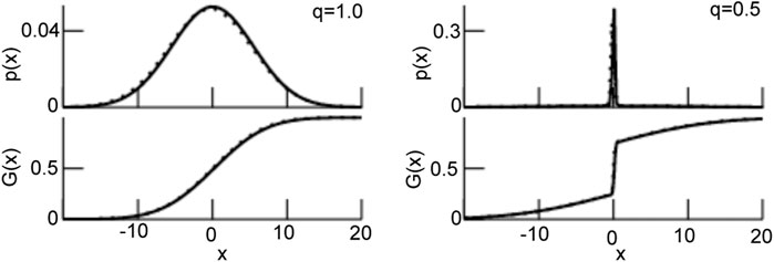
FIGURE 3. The probability density function p (Eq. 26) and the resulting transfer function G (Eq. 27). For $q=1.0$$D_1/{\tau }_e=0.15$ and for $q=0.5$$D_1/{\tau }_e=0.5$.

Essentially, the mean-field obeys

$\begin{array}{l}{\tau }_e\frac{d{a}_1}{dt}=-a_1+F_0{G}_1\left(a_1\right)-M_0{G}_2\left(b_1\right)+I^e+{\rho }^e\left(t\right)\\ {\tau }_i\frac{d{b}_1}{dt}=-b_1+M_0{G}_1\left(a_1\right)-F_0{G}_2\left(b_1\right)+I^i+{\rho }^i\left(t\right)\end{array}(28)$

utilizing (Eq. 27).

3.2 Zero-Mean Gaussian Partial Stimulation

At first, we consider the case of a partial noise stimulation with zero network mean, i.e. ${\mathit{e}}^t{\overline{\mathit{\xi }}}^e=0$ and ${\mathit{s}}_e\left(t\right)\sim \mathcal{N}\left(0,D_1/{\tau }_e{N}_1\right)$ and ${\xi }_1^e={\overline{\xi }}_0^e=0$. Then $D_1$ parametrizes the noise intensity only. Figure 4 shows the network evolution of $\mathit{V}\left(t\right)$ for increasing noise intensities, cf. Equation 7. Starting from a high activity state, increasing the noise intensity yields a phase transition of the system to a network state at lower activity. This occurs for global $\left(q=1.0\right)$ and partial stimulation ($q=0.8$, $q=0.6$ and $q=0.5$). Please re-call that, for instance, $q=0.5$ reflects a stimulation where $50\text{\%}$ of the network nodes are stimulated. These stimulated network nodes have been randomly chosen from a uniform distribution.

FIGURE 4

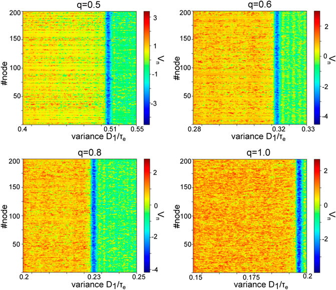
FIGURE 4. Enhanced zero-mean Gaussian noise induces phase transitions in spatiotemporal dynamics. The panels show the network activity $\mathbf{V}\left(\mathrm{t}\right)$ according to Eq. 1 with temporally increasing noise variances $D_1/{\tau }_e$ for different stimulus ratios q.

Figure 5 shows the respective power spectra of the network mean $\mathit{V}\left(t\right)$, which provides insights about the system’s synchronization at low and high noise intensity. High noise intensity induces strong oscillations in the γ-frequency band, whereas the low noise intensity states does not - in contrast, this state shows a decaying low-pass power spectral density that is expected from a non-oscillatory stochastic process.

FIGURE 5

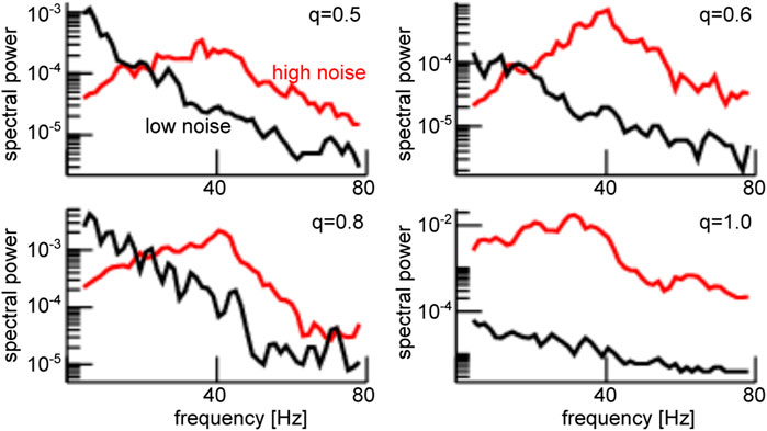
FIGURE 5. Enhanced noise yields strong power of the global mode $\overline{V}\left(t\right)$ in the γ-frequency range. The panels show the power spectra of $\overline{V}$ for the stimulus ratios $q=0.5$ ($D_1/{\tau }_e=0.35$ (black) and $D_1/{\tau }_e=0.55$ (red)), $q=0.6$ ($D_1/{\tau }_e=0.25$ (black) and $D_1/{\tau }_e=0.33$ (red)), $q=0.8$ ($D_1/{\tau }_e=0.20$ (black) and $D_1/{\tau }_e=0.25$ (red)) and $q=1.0$ ($D_1/{\tau }_e=0.15$ (black) and $D_1/{\tau }_e=0.20$ (red)). Power spectra at lower noise intensities are computed on the respective upper branch of the bistable system.

Stronger power spectral density at a given frequency is the signature of a coherent network, as seen in Figure 5. Since the neurons in our network model emit spikes and exhibit synaptic input currents, noise-induced coherence may be visible in the coherence between spiking and synaptic activity as well. In fact, in Figure 6A one observes a significant strongly enhanced Spike Field Coherence at high noise intensities for both global and partial stimulation. Hence, in sum the system exhibits coherence resonance in the sense that strong noise induces coherent oscillations that are not present at low noise intensities.

FIGURE 6

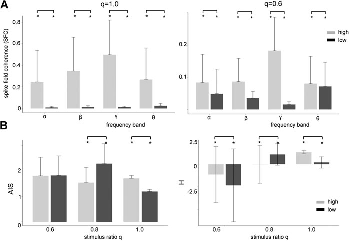
FIGURE 6. High zero-mean Gaussian noise enhances the Spike Field Coherence in all frequency bands and affects heterogeneously Active Information Storage (AIS) and differential entropy (H). (A) The differences between high noise intensity (grey-colored) and low noise intensity (black-colored) is significant $\left(p<0.001\right)$ for both global and partial stimulation. (B) For global stimulation $\left(q=1.0\right)$, high noise intensity induces states of significantly enhanced stored active information (AIS) and available information (H), whereas partial stimulation with $q=0.8$ diminishes both AIS and H significantly. Results for $q=0.6$ are not consistent and difficult to interpret. In all panels, vertical bars denote the standard deviation, $p<0.001$ and parameters are identical to the parameters used in Figure 5.

Coherence resonance is supposed to be linked to information processing in neural systems. Thus we investigate the relationship between stimulus noise intensity and information in the system across frequency bands. Figure 6B shows how much information is stored in the networks (AIS) and how much information is available (H). We observe that significantly more information is stored (AIS) and available (H) at high noise intensities for global stimulation $q=1.0$, whereas high noise partial stimulation with $q=0.8$ diminishes the stored active information and available information significantly. For more sparse stimulation with $q=0.6$ the finding in information measures is heterogeneous and no interpretation consistent with the results for larger q is possible.

To understand this noise-induced coherence, we take a closer look at the dynamic topology of the mean-field Eq. 28. Their equilibria (cf. section 2.3) for negligible finite-size fluctuations ${\rho }^{e,i}\left(t\right)\ll 1$ are shown in Figure 7 together with simulated mean-field activity $\overline{V}\left(t\right)$ for illustrative purposes. Low noise intensity induces a bistable regime with a stable node as upper equilibrium and a focus as lower equilibrium. For global stimulation ($q=1.0$), this lower focus is unstable at very low noise intensity and stable at larger noise intensities. Moreover, the lower equilibrium is a stable focus at all noise intensities for partial ($q<1.0$) stimulation. The center branch is always a saddle node. For larger noise intensity, the upper equilibrium branch merges with the center branch via a saddle-node bifurcation and the lower stable focus is preserved as noise is further increased. This finding remains valid for both global ($q=1.0$) and partial ($q<1.0$) stimulation as shown in Figure 7 for q ranging within the interval $0.5\le q\le 1.0$. One can see that for smaller q (i.e. less excitatory neurons are stimulated) the bifurcation point moves to larger noise intensities. Hence thinning out the stimulation of excitatory neurons increases the noise intensity interval at which bistability occurs. Moreover, we point out that the bifurcation points predicted by the mean-field description and shown in Figure 7 show very good accordance to the values of $D_1/{\tau }_e$ in Figure 4, where the system transitions from the upper to the lower state.

FIGURE 7

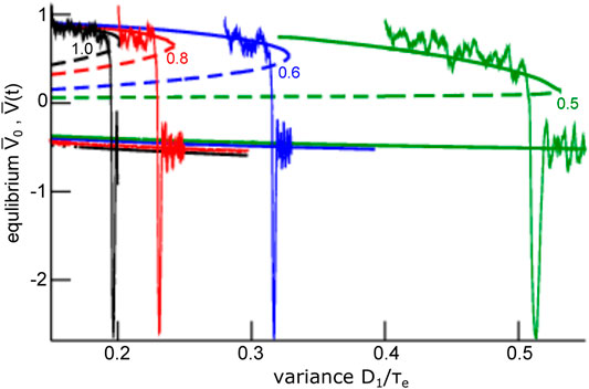
FIGURE 7. Equilibria and representative time series of the global mode $\overline{V}\left(t\right)$ for the zero-mean partial stimulation. There is a bistability and saddle-node bifurcation from a stable node to an stable focus at enhanced noise intensity. The numbers denote the values of the stimulus ratio q. Solid (dashed) lines mark stable (unstable) states. The time series $\overline{V}$ results from the time-varying noise intensity according to Eq. 7.

The mean-field solution involves finite-size fluctuations that affect the solutions principal oscillation frequency and magnitude. By construction, these mean-field solutions converge to the network average for increasing network size N. Figure 8 compares the time series of mean-field solutions and network averages for increasing network sizes and affirms the convergence and thus the validity of the mean-field description. It is interesting to note that, besides the mean-field dynamics, the network’s dynamical properties change with increasing N as well. Figure 8 provides the principal oscillation frequencies for both solutions for the given network size: the network speeds up with increasing size and its frequency converges to the mean-field principal frequency that remains about the same value. However, we point out that the mean-field solution remains still slightly different even for very large N since it implies the approximation of negligible connectivity matrix bulk spectra. Figure 9 affirms this finding by comparing simulation trials of the transitions from the non-oscillatory to the oscillatory coherent state. We observe that the transition values of $D_1/{\tau }_e$ of the network mean and the mean-field are closer to each other for larger network size. The mean-field description (Eq. 28) with (Eq. 27) assumes vanishing finite-size fluctuations and these are reduced for larger network size N, i.e. the effective noise level (the finite-size fluctuations) is reduced and thus deterministic mean-field and stochastic network activity transition are closer to each other.

FIGURE 8

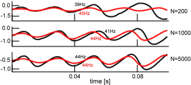
FIGURE 8. Comparison of network average and mean-field solution for different network sizes. The network average (black) and mean-field solutions (red) resembles more and more the larger the network of size N. This holds for the magnitude and frequency (provided in panels) of both solutions. The initial value of the mean-field activity has been chosen to the initial value of the network average. Simulations consider zero-mean Gaussian simulations with $q=1$ and $D_1/{\tau }_e=0.2$.

FIGURE 9

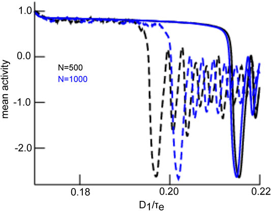
FIGURE 9. Comparison of transitions in network and mean-field for different network sizes. The network average (dashed line) and mean-field solutions (solid line) resemble more for larger network size N. This is explained by reduced finite-size fluctuations for larger networks. The initial value of the mean-field activity has been chosen to the initial value of the network average. Simulations consider zero-mean Gaussian simulations with $q=1$.

The frequency range of oscillations observed for steady states located within the lower branch (see Figure 7) is a consequence of both network connectivity and neuronal properties and is further tuned by additive noise. Figure 10 shows the maximum eigenvalue real part for the upper (A) and the lower branch (B, top opanel) and the eigenfrequency (cf. section 2.3) of the equilibrium at the lower branch (B, lowel panel). We observe that increasing noise intensity decreases slightly the eigenfrequency in the $\gamma -$ frequency range and decreases the negative maximum eigenvalue real part. This means that additive noise increases the damping of the response of the system to perturbations - including noise. This increased noise-induced damping leads to magnitude changes in quasi-cycle solutions - which is manifested in the power spectral density distribution. Indeed, the power spectral density distribution widens as noise intensity increases, leading to the spectra as seen in Figure 10C. This broad spectral power distribution is the signature of suppressed coherence. As a corollary, our analysis demonstrates that coherent band-limited oscillations emerge for intermediate noise intensities only. This is a known feature of coherence resonance. For additional illustration, Figure 1 shows the typical bell-shape of coherence (here Spike Field Coherence) in different frequency bands. We observe that the coherence effect is strongest in the $\gamma -$ frequency range.

FIGURE 10

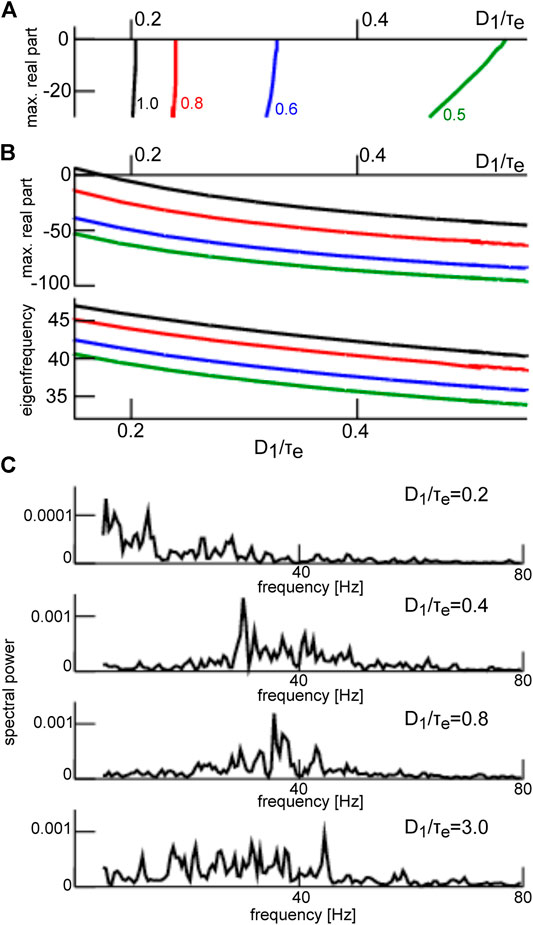
FIGURE 10. Eigenvalues at the top and bottom branch in Figure 7 and corresponding power spectra. (A) maximum eigenvalue of equilibria on the top branch in Figure 7. (B) maximum real part r of the eigenvalue $r+i2\pi \nu$ (top panel) and the corresponding eigenfrequency frequency ν. The numbers denote the values of the stimulus ratio q in all panels. (C) Power spectra of $\mathit{V}\left(t\right)$ about the lower branch for $q=0.6$ for different noise intensities $D_1/{\tau }_e$.

3.3 Poisson Partial Stimulation

Synaptic receptors respond to afferent Poisson-distributed input spike trains, whose properties differ substantially from the Gaussian noise processes we considered so far. To generalize our results to more physiological stimuli statistics, we considered a partial Poisson noise stimulation with dependent mean and variance. Specifically, afferent spike trains at spike rate $r_{\text{in}}$ induce random responses at excitatory synapses with time constant ${\tau }_{\text{in}}$ and synaptic weight $w_{\text{in}}$. Then

${\mathit{s}}^e\left(t\right)={\tau }_e\text{Δ}\mathit{\xi }+{\overline{\rho }}^e\left(t\right)$

${\xi }_1^e=w_{\text{in}}{r}_{\text{in}}{\tau }_{\text{in}}$

$D_1=w_{\text{in}}{\xi }_0/2$

${\overline{\xi }}_0^e=q{\xi }_1^e,$

and finite-size fluctuations ${\overline{\rho }}^e\left(t\right)\sim \mathcal{N}\left(0,D_1/N_1\right)$. Figure 11A illustrates the temporal network activity for a low and high stimuli firing rates $r_{\text{in}}$. Increasing $r_{\text{in}}$ induces a transition from a high-activity to a low activity state for both global and partial stimulation - similarly as in the Gaussian noise case. The high-activity state is non-oscillatory while the low-activity state is oscillatory, with frequency found in the $\gamma -$ frequency range (Figure 11B). In addition, the low-activity state induced by high Poisson input rate exhibits a strong Spike Field Coherence in contrast to the high-activity state (Figure 11C). Moreover, high stimulation noise increases the stored information and the available information for global stimulation with $q=1.0$, cf. Figure 11D. Information measures for partial stimulation $\left(q=0.6\right)$ are heterogeneous and an interpretation of results for AIS and H is difficult.

FIGURE 11

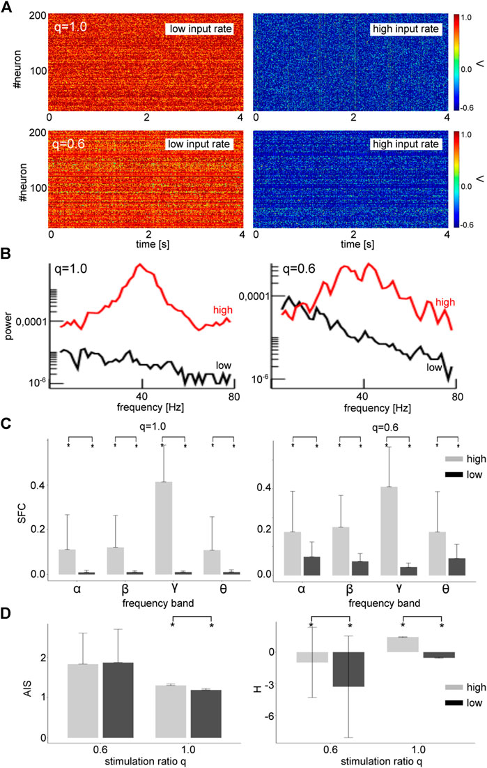
FIGURE 11. Poisson noise induces transitions from a non-oscillatory to an oscillatory state for both global and partial stimulation. (A) Network activity $V_n\left(t\right)$ for low input firing rate ($r=0.04$ for $q=1.0$ and $r=0.09$ for $q=0.6$) and high input firing rate ($r=0.14$ for $q=1.0$ and $r=0.19$ for $q=0.6$). For the low (high) input rate the system evolves about an upper (lower) state. (B) Power spectra of the network mean $\overline{V}\left(t\right)$ showing $\gamma -$ activity for the large input rate. (C) The high input firing rate (grey-colored) induces a state of large Spike Field Coherence compared to the state for low input firing rate (black-colored) for both global and partial stimulation ($p<0.01$). (D) For global stimulation ($q=1.0$), high input firing induces a state of significantly enhanced stored active information ($AIS$) and available information (H). This is not consistent to results for partial stimulation $\left(q=0.6\right)$. Here is $p<0.01$.

These results can be understood by taking a closer look at the dynamic topology of the system. Figure 12 reveals that, for global stimulation $\left(q=1.0\right)$, the system has two unstable equilibria and one stable equilibrium at lower noise intensities. The top branch is a stable node, the center branch a saddle node and the lower branch an unstable focus. There is a very small noise intensity interval at which the top and bottom branch are both stable. Increasing the Poisson stimuli firing rate leads to a sudden suppression of high-activity equilibria through a saddle-node bifurcation. Consequently, the transition observed in Figure 11A is a jump from the stable node on the top bifurcation branch to the stable focus on the bottom branch similar to the effect shown in Figure 4. For partial stimulation $\left(q=0.6\right)$, the lower branch exhibits a stable focus for much lower input firing rates. The saddle-node bifurcation is delayed, leading to an increased noise intensity interval of bistability. Hence, the system exhibits coherence resonance for Poisson noise as well.

FIGURE 12

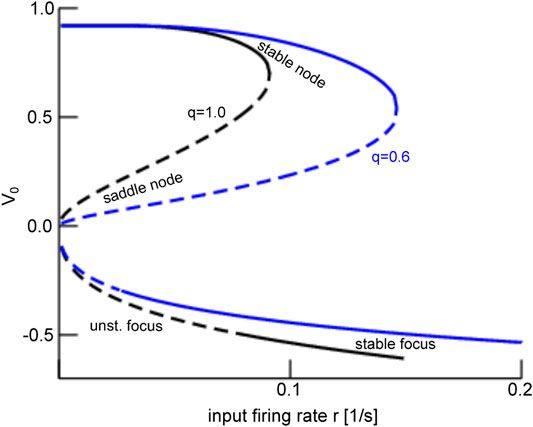
FIGURE 12. Equilibria of the mean-field $\overline{V}\left(t\right)$ for the Poisson partial stimulation. For global stimulation $q=1.0$, the system is always monostable with three equilibria at low input firing rates and a single equilibrium at large input firing rates. Increasing the input firing rate from low to large firing rates, the system jumps from the upper stationary state (stable node) to a stable focus on the lower stationary state via a saddle-node bifurcation. For partial stimulation $q=0.6$, the system is monostable with three equilibria at low input firing rates. For larger input rates, the system is bistable and passes a saddle-node bifurcation inducing a transition from a stable node to an stable focus at enhanced input firing rate r. Solid (dashed) lines mark stable (unstable) states, black- and blue-colored lines denote equilibria for global and partial stimulation, respectively. The bifurcation diagram of the mean-field $\overline{W}\left(t\right)$ is equivalent.

4 Discussion

This study presents a rigorous derivation of mean-field equations for two nonlinearly coupled non-sparse Erdös-Rényi networks (ERN) that are stimulated by additive noise. This mean field representation is made possible through spectral separation: the eigenspectrum of ERN networks exhibits a large spectral gap between the eigenvalue with largest real part and the rest of the spectrum. We show that the projection of the network dynamics onto the leading eigenmode represents the mean-field. Its dynamics are shaped by eigenmodes located in the complement subspace spanned by non-leading eigenmodes. In our model, the subspace dynamics are governed and influenced by additive noise statistics and they obey an Ornstein-Uhlenbeck process.

We extended the mean-field derivation to various types of additive noise, such as global and partial noise stimuli (i.e. when only a fraction of the excitatory neurons are stimulated) and for both zero-mean Gaussian and Poisson-like noise. Collectively, our analysis shows that additive noise induces a phase transition from a non-oscillatory state to an oscillatory coherent state. Such noise-induced coherence is known as coherence resonance (CR). This phase transition has been shown to occur not only for Gaussian zero-mean noise but also for Poisson-like noise. To the best of our knowledge, CR has not been found yet for such Poisson-like noise. The general underlying mechanism is a noise-induced multiplicative impact of additive stimulation via the nonlinear coupling of different modes. This multiplicative effect modifies the net transfer function of the network and thus enlarges its dynamical repertoire. This resembles the impact of additive noise in stochastic bifurcations [51, 52, 70, 71].

Embedding into Literature

Our results build on previous studies from the authors [23, 54, 55] to provide a rigorous derivation of the mean-field description, whereas previous work have motivated heuristically the mean-field reduction and, e.g., failed to show in detail whether the mean-field equation is the only solution for any given additive stimuli. Several other previous studies have presented mean-field descriptions in stochastically driven systems. For instance, Bressloff et al. [28] have derived rigorously mean-field equations for stochastic neural fields considering, inter alia, finite-element fluctuations by utilizing a Master equation and van Kampen’s volume expansion approach. We note here that we also took into account finite-size fluctuations resulting from a non-negligible variance of statistical mean values. Moreover [28], do not specify the network type and results in a rather opaque description, whereas we assume an ERN and thus exploit its unique eigenspectrum structure. This yields directly to a mean-field description, whose dependence of stochastic forces is obvious and avoids its implicit closure problem known from mean-field theories [43]. This is possible since the ERN considered share many properties with Izing models, that are known to permit an analytically treatable solution of the closure problem, see e.g. [72].

Moreover, several technical analysis steps in the present work have been applied in previous studies in a similar context. In a work on stochastic neural mean-field theory, Faugeras and others [27] have assumed that the system activity fluctuations obey a normal probability distribution and have derived an effective nonlinear interaction in their Proposition 2.1 similar to our Eq. 22. Further, the authors have shown how the fluctuation correlation function, i.e. the system activity’s second moment, determine the mean-field dynamics. This is in line with our result (Eq. 22) showing how the mean and variance of the additive noise tunes the system’s stability. However, the authors have not considered in detail the random nature of the system connectivity, whereas we have worked out the interaction of external stimulation and the ERN. This interaction yields directly the mean-field and its dependence of the external stimulus that is not present in [27]. Moreover, the present work also shows how the mean-field fluctuations affect the mean-field dynamics by deriving the fluctuation’s probability density function that describes all higher moments.

Noise-induced synchronization has been found recently in a system of stochastically driven linearly coupled FitzHugh-Nagumo neurons by Touboul and others [73]. The authors have found a minimum ratio of activated neurons that are necessary to induce global oscillatory synchronization, i.e. CR in the sense presented in our work. This question has been considered in the present work as well by asking how the mean-field dynamics, and thus how noise-induced synchronization, changes when modifying the ratio of stimulated excitatory neurons q while retaining the stimulation of inhibitory neurons. We find that global stimulation, i.e. stimulation of all excitatory neurons, yields a finite critical noise intensity below which the system is bistable and exhibits CR. Partial stimulation shifts this critical noise intensity to larger values and enlarges the bistability parameter space and thus promotes CR.

Several previous studies of mean-field dynamics in neural systems have applied the master equation formalism [74–76]. This works nicely in completely irregular networks and the asynchronous activity regime and has been applied successfully to neural populations considering biological neuron models [77–80]. However, the analysis of more regular networks will be very difficult to develop with the Master equation since the implicit integration over system states would be more complex. Conversely, our presented approach may consider regular structures by a corresponding matrix eigenvalue decomposition.

At last, we mention the relation to the Master stability function [81, 82]. This function describes the stability of identical synchronization of complex networks in a synchronization manifold and this manifold corresponds to the mean-field in our study. Although the Master stability function has been proven to be powerful, to the best of our knowledge it does not allow to reveal coherence resonance as the current work.

Limits and Outlook

The present work proposes to describe mean-field dynamics in a topological network by projection onto the networks eigenmodes. This works well for non-sparse random ERN with large connectivity probability. This network does not exhibit a spatial structure. However, less connected ERN networks show different dynamics, cf. the Supplementary Appendix. Moreover, biological networks are not purely random but may exhibit distance-dependent synaptic weights [83] or spatial clusters [84]. Our specific analysis applies for networks with a large spectral gap in their eigenspectra and it might fail for biological networks with smaller spectral gaps (as shown in the Supplementary Appendix). Future work will attempt to utilize the presented approach to derive mean-field dynamics for heterogeneous networks that exhibit a smaller spectral gap, such as scale-free networks [84].

Moreover, the single neuron model in the present work assumes a simple static threshold firing dynamics (McCullough-Pitts neuron) while neglecting somatic dynamics as described by Hodgkin-Huxley type models or the widely used FitzHugh-Nagumo model [11, 73]. Future work will aim at reinforcing the biological relevance of neurons coupled through ERN. This will be possible by extending the trivial transfer function from a step function to sigmoidal shapes for type I or type II neurons [76, 85, 86].

Our results show that noise-induced CR emerges in the $\gamma -$ frequency range. This frequency band is thought to play an important role in visual information processing [13–17]. Experimental studies have shown that the degree of this γ-synchronization in primary cortical areas may be modulated by attention [59, 87–89]. Since attention is known to affect the ARAS activity [90] and specifically the brain stem as part of the ARAS [91] and ARAS, in turn, provides input to the cortex [92]. We conclude that it is possible that attention modulates the cortical input activity, i.e. the Poisson firing rate in our model. In this picture, attention-modulated enhanced ARAS activity induces $\gamma -$ coherence and may enhance stored information [93], as shown in Figures 6, 11. Future more detailed brain models including the cortico-thalamic feedback and cortical interactions [21, 57] will provide further evidence whether coherence resonance is present in visual processing.

Data Availability Statement

The raw data supporting the conclusion of this article will be made available by the authors, without undue reservation.

Author Contributions

AH conceived the work structure motivated by intensive discussions with JL; AH, TW, NV, and JH contributed different work parts and all authors have written the work.

Conflict of Interest

JH was employed by Hyland Switzerland Sarl.

The remaining authors declare that the research was conducted in the absence of any commercial or financial relationships that could be construed as a potential conflict of interest.

Supplementary Material

The Supplementary Material for this article can be found online at: https://www.frontiersin.org/articles/10.3389/fams.2021.697904/full#supplementary-material

References

1. Pikovsky, A, Rosenblum, M, and Kurths, J. Synchronization: A Universal Concept in Nonlinear Sciences. Cambridge University Press (2001).

2. Singer, W. The Brain as a Self-Organizing System. Eur Arch Psychiatr Neurol Sci (1986) 236:4–9. doi:10.1007/bf00641050

CrossRef Full Text | Google Scholar

3. Witthaut, D, Wimberger, S, Burioni, R, and Timme, M. Classical Synchronization Indicates Persistent Entanglement in Isolated Quantum Systems. Nat Commun (2017) 8:14829. doi:10.1038/ncomms14829

PubMed Abstract | CrossRef Full Text | Google Scholar

4. Hutt, A, and Haken, H. Synergetics. New York: Springer-Verlag (2020).

5. Mompo, E, Ruiz-Garcia, M, Carretero, M, Grahn, HT, Zhang, Y, and Bonilla, LL. Coherence Resonance and Stochastic Resonance in an Excitable Semiconductor Superlattice. Phys Rev Lett (2018) 121:086805. doi:10.1103/PhysRevLett.121.086805

PubMed Abstract | CrossRef Full Text | Google Scholar

6. Lee, CY, Choi, W, Han, J-H, and Strano, MS. Coherence Resonance in a Single-Walled Carbon Nanotube Ion Channel. Science (2010) 329:1320–4. doi:10.1126/science.1193383

PubMed Abstract | CrossRef Full Text | Google Scholar

7. Gu, H, Yang, M, Li, L, Liu, Z, and Ren, W. Experimental Observation of the Stochastic Bursting Caused by Coherence Resonance in a Neural Pacemaker. Neuroreport (2002) 13:1657–60. doi:10.1097/00001756-200209160-00018

PubMed Abstract | CrossRef Full Text | Google Scholar

8. Ratas, I, and Pyragas, K. Noise-induced Macroscopic Oscillations in a Network of Synaptically Coupled Quadratic Integrate-And-Fire Neurons. Phys Rev E (2019) 100:052211. doi:10.1103/PhysRevE.100.052211

PubMed Abstract | CrossRef Full Text | Google Scholar

9. Pikovsky, AS, and Kurths, J. Coherence Resonance in a Noise-Driven Excitable System. Phys Rev Lett (1997) 78:775–8. doi:10.1103/physrevlett.78.775

CrossRef Full Text | Google Scholar

10. Gang, H, Ditzinger, T, Ning, CZ, and Haken, H. Stochastic Resonance without External Periodic Force. Phys Rev Lett (1993) 71:807–10. doi:10.1103/physrevlett.71.807

PubMed Abstract | CrossRef Full Text | Google Scholar

11. Baspinar, E, Schüler, L, Olmi, S, and Zakharova, A. Coherence Resonance in Neuronal Populations: Mean-Field versus Network Model. Submitted (2020).

12. Tönjes, R, Fiore, CE, and Pereira, T. Coherence Resonance in Influencer Networks. Nat Commun (2021) 12:72. doi:10.1038/s41467-020-20441-4

PubMed Abstract | CrossRef Full Text | Google Scholar

13. Singer, W, and Gray, CM. Visual Feature Integration and the Temporal Correlation Hypothesis. Annu Rev Neurosci (1995) 18:555–86. doi:10.1146/annurev.ne.18.030195.003011

PubMed Abstract | CrossRef Full Text | Google Scholar

14. Eckhorn, R, Bauer, R, Jordan, W, Brosch, M, Kruse, W, Munk, M, et al. Coherent Oscillations: A Mechanism of Feature Linking in the Visual Cortex? Biol Cybern (1988) 60:121–30. doi:10.1007/bf00202899

PubMed Abstract | CrossRef Full Text | Google Scholar

15. Castelo-Branco, M, Neuenschwander, S, and Singer, W. Synchronization of Visual Responses between the Cortex, Lateral Geniculate Nucleus, and Retina in the Anesthetized Cat. J Neurosci (1998) 18:6395–410. doi:10.1523/jneurosci.18-16-06395.1998

CrossRef Full Text | Google Scholar

16. Nelson, JI, Salin, PA, Munk, MH-J, Arzi, M, and Bullier, J. Spatial and Temporal Coherence in Cortico-Cortical Connections: a Cross-Correlation Study in Areas 17 and 18 in the Cat. Vis Neurosci (1992) 9:21–37. doi:10.1017/s0952523800006349

PubMed Abstract | CrossRef Full Text | Google Scholar

17. Bressler, SL. Interareal Synchronization in the Visual Cortex. Behav Brain Res (1996) 76:37–49. doi:10.1016/0166-4328(95)00187-5

PubMed Abstract | CrossRef Full Text | Google Scholar

18. Munk, MHJ, Roelfsema, PR, Konig, P, Engel, AK, and Singer, W. Role of Reticular Activation in the Modulation of Intracortical Synchronization. Science (1996) 272:271–4. doi:10.1126/science.272.5259.271

PubMed Abstract | CrossRef Full Text | Google Scholar

19. Hutt, A, Lefebvre, J, Hight, D, and Sleigh, J. Suppression of Underlying Neuronal Fluctuations Mediates EEG Slowing during General Anaesthesia. Neuroimage (2018) 179:414–28. doi:10.1016/j.neuroimage.2018.06.043

PubMed Abstract | CrossRef Full Text | Google Scholar

20. Hutt, A. Cortico-thalamic Circuit Model for Bottom-Up and Top-Down Mechanisms in General Anesthesia Involving the Reticular Activating System. Arch Neurosci (2019) 6:e95498. doi:10.5812/ans.95498

CrossRef Full Text | Google Scholar

21. Hutt, A, and Lefebvre, J. Arousal Fluctuations Govern Oscillatory Transitions between Dominant γ- and α Occipital Activity during Eyes Open/Closed Conditions. Brain Topography (2021), in press.

Google Scholar

22. Pisarchik, AN, Maksimenko, VA, Andreev, AV, Frolov, NS, Makarov, VV, Zhuravlev, MO, et al. Coherent Resonance in the Distributed Cortical Network during Sensory Information Processing. Sci Rep (2019) 9:18325. doi:10.1038/s41598-019-54577-1

PubMed Abstract | CrossRef Full Text | Google Scholar

23. Hutt, A, Lefebvre, J, Hight, D, and Kaiser, HA. Phase Coherence Induced by Additive Gaussian and Non-gaussian Noise in Excitable Networks with Application to Burst Suppression-like Brain Signals. Front Appl Math Stat (2020) 5:69. doi:10.3389/fams.2019.00069

CrossRef Full Text | Google Scholar

24. Chacron, MJ, Longtin, A, and Maler, L. The Effects of Spontaneous Activity, Background Noise, and the Stimulus Ensemble on Information Transfer in Neurons. Netw Comput Neural Syst (2003) 14:803–24. doi:10.1088/0954-898x_14_4_010

CrossRef Full Text | Google Scholar

25. Chacron, MJ, Lindner, B, and Longtin, A. Noise Shaping by Interval Correlations Increases Information Transfer. Phys.Rev.Lett. (2004) 93:059904. doi:10.1103/physrevlett.93.059904

CrossRef Full Text | Google Scholar

26. Chacron, MJ, doiron, B, Maler, L, Longtin, A, and Bastian, J. Non-classical Receptive Field Mediates Switch in a Sensory Neuron's Frequency Tuning. Nature (2003) 423:77–81. doi:10.1038/nature01590

PubMed Abstract | CrossRef Full Text | Google Scholar

27. Faugeras, OD, Touboul, JD, and Cessac, B. A Constructive Mean-Field Analysis of Multi Population Neural Networks with Random Synaptic Weights and Stochastic Inputs. Front Comput Neurosci (2008) 3:1. doi:10.3389/neuro.10.001.2009

CrossRef Full Text | Google Scholar

28. Bressloff, PC. Stochastic Neural Field Theory and the System Size Expansion. SIAM J Appl Math (2009) 70:1488–521.

Google Scholar

29. Terney, D, Chaieb, L, Moliadze, V, Antal, A, and Paulus, W. Increasing Human Brain Excitability by Transcranial High-Frequency Random Noise Stimulation. J Neurosci (2008) 28:14147–55. doi:10.1523/jneurosci.4248-08.2008

CrossRef Full Text | Google Scholar

30. Erdős, L, Knowles, A, Yau, H-T, and Yin, J. Spectral Statistics of Erdős-Rényi Graphs I: Local Semicircle Law. Ann Probab (2013) 41:2279–375. doi:10.1214/11-AOP734

CrossRef Full Text | Google Scholar

31. Ding, X, and Jiang, T. Spectral Distributions of Adjacency and Laplacian Matrices of Random Graphs. Ann Appl Prob (2010) 20:2086–117. doi:10.1214/10-aap677

CrossRef Full Text | Google Scholar

32. Kadavankandy, A. Spectral Analysis of Random Graphs with Application to Clustering and Sampling. In: Ph.D. Thesis, Université Cote d’Azur. Nice, France: NNT: 2017AZUR4059 (2017).

Google Scholar

33. Füredi, Z, and Komlós, J. The Eigenvalues of Random Symmetric Matrices. Combinatorica (1981) 1:233–41. doi:10.1007/bf02579329

CrossRef Full Text | Google Scholar

34. O'Rourke, S, Vu, V, and Wang, K. Eigenvectors of Random Matrices: A Survey. J Comb Theor Ser A (2016) 144:361–442. doi:10.1016/j.jcta.2016.06.008

CrossRef Full Text | Google Scholar

35. Koch, C. Biophysics of Computation. Oxford: Oxford University Press (1999).

36. Ross, S. Stochastic Processes (Probability and Mathemati- Cal Statistics). Wiley (1982).

37. Wright, JJ, and Kydd, RR. The Electroencephalogram and Cortical Neural Networks. Netw Comput Neural Syst (1992) 3:341–62. doi:10.1088/0954-898x_3_3_006

CrossRef Full Text | Google Scholar

38. Nunez, PL. Toward a Quantitative Description of Large-Scale Neocortical Dynamic Function and EEG. Behav Brain Sci (2000) 23:371–98. doi:10.1017/s0140525x00003253

PubMed Abstract | CrossRef Full Text | Google Scholar

39. Nunez, P, and Srinivasan, R. Electric Fields of the Brain: The Neurophysics of EEG. New York - Oxford: Oxford University Press (2006).

40. Wilson, HR, and Cowan, JD. Excitatory and Inhibitory Interactions in Localized Populations of Model Neurons. Biophysical J (1972) 12:1–24. doi:10.1016/s0006-3495(72)86068-5

CrossRef Full Text | Google Scholar

41. Gerstner, W, and Kistler, W. Spiking Neuron Models. Cambridge: Cambridge University Press (2002).

42. Bressloff, PC, and Coombes, S. Physics of the Extended Neuron. Int J Mod Phys B (1997) 11:2343–92. doi:10.1142/s0217979297001209

CrossRef Full Text | Google Scholar

43. Kuehn, C. Moment Closure-A Brief Review. In: Schöll E, Klapp S, and Hövel P, editors. Control of Self-Organizing Nonlinear Systems. Heidelberg: Springer (2016). p. 253–71. doi:10.1007/978-3-319-28028-8_13

CrossRef Full Text | Google Scholar

44. Sri Namachchivaya, N. Stochastic Bifurcation. Appl Math Comput (1990) 39:37s–95s. doi:10.1016/0096-3003(90)90003-L

CrossRef Full Text | Google Scholar

45. Berglund, N, and Gentz, B. Geometric Singular Perturbation Theory for Stochastic Differential Equations. J Differential Equations (2003) 191:1–54. doi:10.1016/s0022-0396(03)00020-2

CrossRef Full Text | Google Scholar

46. Bloemker, D, Hairer, M, and Pavliotis, GA. Modulation Equations: Stochastic Bifurcation in Large Domains. Commun Math Phys (2005) 258:479–512. doi:10.1007/s00220-005-1368-8

CrossRef Full Text | Google Scholar

47. Boxler, P. A Stochastic Version of center Manifold Theory. Probab Th Rel Fields (1989) 83:509–45. doi:10.1007/bf01845701

CrossRef Full Text | Google Scholar

48. Hutt, A, and Lefebvre, J. Stochastic center Manifold Analysis in Scalar Nonlinear Systems Involving Distributed Delays and Additive Noise. Markov Proc Rel Fields (2016) 22:555–72.

Google Scholar

49. Lefebvre, J, Hutt, A, LeBlanc, VG, and Longtin, A. Reduced Dynamics for Delayed Systems with Harmonic or Stochastic Forcing. Chaos (2012) 22:043121. doi:10.1063/1.4760250

PubMed Abstract | CrossRef Full Text | Google Scholar

50. Hutt, A. Additive Noise May Change the Stability of Nonlinear Systems. Europhys Lett (2008) 84:34003. doi:10.1209/0295-5075/84/34003

CrossRef Full Text | Google Scholar

51. Hutt, A, Longtin, A, and Schimansky-Geier, L. Additive Noise-Induced Turing Transitions in Spatial Systems with Application to Neural fields and the Swift-Hohenberg Equation. Physica D: Nonlinear Phenomena (2008) 237:755–73. doi:10.1016/j.physd.2007.10.013

CrossRef Full Text | Google Scholar

52. Hutt, A, Longtin, A, and Schimansky-Geier, L. Additive Global Noise Delays Turing Bifurcations. Phys Rev Lett (2007) 98:230601. doi:10.1103/physrevlett.98.230601

PubMed Abstract | CrossRef Full Text | Google Scholar

53. Hutt, A, and Lefebvre, J. Additive Noise Tunes the Self-Organization in Complex Systems. In: Hutt A, and Haken H, editors. Synergetics, Encyclopedia of Complexity and Systems Science Series. New York: Springer (2020). p. 183–95. doi:10.1007/978-1-0716-0421-2_696

CrossRef Full Text | Google Scholar

54. Lefebvre, J, Hutt, A, Knebel, J-F, Whittingstall, K, and Murray, MM. Stimulus Statistics Shape Oscillations in Nonlinear Recurrent Neural Networks. J Neurosci (2015) 35:2895–903. doi:10.1523/jneurosci.3609-14.2015

CrossRef Full Text | Google Scholar

55. Hutt, A, Mierau, A, and Lefebvre, J. Dynamic Control of Synchronous Activity in Networks of Spiking Neurons. PLoS One (2016) 11:e0161488. doi:10.1371/journal.pone.0161488

PubMed Abstract | CrossRef Full Text | Google Scholar

56. Hutt, A, Sutherland, C, and Longtin, A. Driving Neural Oscillations with Correlated Spatial Input and Topographic Feedback. Phys.Rev.E (2008) 78:021911. doi:10.1103/physreve.78.021911

PubMed Abstract | CrossRef Full Text | Google Scholar

57. Hashemi, M, Hutt, A, and Sleigh, J. How the Cortico-Thalamic Feedback Affects the EEG Power Spectrum over Frontal and Occipital Regions during Propofol-Induced Sedation. J Comput Neurosci (2015) 39:155–79. doi:10.1007/s10827-015-0569-1

CrossRef Full Text | Google Scholar

58. Klöden, PE, and Platen, E. Numerical Solution of Stochastic Differential Equations. Heidelberg: Springer-Verlag (1992).

59. Fries, P, Reynolds, J, Rorie, A, and Desimone, R. Modulation of Oscillatory Neuronal Synchronization by Selective Visual Attention. Science (2001) 291:1560–3. doi:10.1126/science.1055465

PubMed Abstract | CrossRef Full Text | Google Scholar

60. Tononi, G. An Information Integration Theory of Consciousness. BMC Neurosci (2004) 5:42. doi:10.1186/1471-2202-5-42

PubMed Abstract | CrossRef Full Text | Google Scholar

61. Alkire, MT, Hudetz, AG, and Tononi, G. Consciousness and Anesthesia. Science (2008) 322:876–80. doi:10.1126/science.1149213

PubMed Abstract | CrossRef Full Text | Google Scholar

62. Lee, M, Sanders, RD, Yeom, S-K, Won, D-O, Seo, K-S, Kim, HJ, et al. Network Properties in Transitions of Consciousness during Propofol-Induced Sedation. Sci Rep (2017) 7:16791. doi:10.1038/s41598-017-15082-5

PubMed Abstract | CrossRef Full Text | Google Scholar

63. Massimini, M, Ferrarelli, F, Huber, R, Esser, SK, Singh, H, and Tononi, G. Breakdown of Cortical Effective Connectivity during Sleep. Science (2005) 309:2228–32. doi:10.1126/science.1117256

PubMed Abstract | CrossRef Full Text | Google Scholar

64. Wollstadt, P, Sellers, KK, Rudelt, L, Priesemann, V, Hutt, A, Fröhlich, F, et al. Breakdown of Local Information Processing May Underlie Isoflurane Anesthesia Effects. Plos Comput Biol (2017) 13:e1005511. doi:10.1371/journal.pcbi.1005511

PubMed Abstract | CrossRef Full Text | Google Scholar

65. Lizier, JT, Prokopenko, M, and Zomaya, AY. Local Measures of Information Storage in Complex Distributed Computation. Inf Sci (2012) 208:39–54. doi:10.1016/j.ins.2012.04.016

CrossRef Full Text | Google Scholar

66. Wibral, M, Lizier, JT, Vögler, S, Priesemann, V, and Galuske, R. Local Active Information Storage as a Tool to Understand Distributed Neural Information Processing. Front Neuroinform (2014) 8:1. doi:10.3389/fninf.2014.00001

PubMed Abstract | CrossRef Full Text | Google Scholar

67. Ince, RAA, Giordano, BL, Kayser, C, Rousselet, GA, Gross, J, and Schyns, PG. A Statistical Framework for Neuroimaging Data Analysis Based on Mutual Information Estimated via a Gaussian Copula. Hum Brain Mapp (2017) 38:1541–73. doi:10.1002/hbm.23471

PubMed Abstract | CrossRef Full Text | Google Scholar

68. Wibral, M, Pampu, N, Priesemann, V, Siebenhühner, F, Seiwert, H, Lindner, RV, et al. Measuring Information-Transfer Delays. PLoS One (2013) 8:e55809. doi:10.1371/journal.pone.0055809

PubMed Abstract | CrossRef Full Text | Google Scholar

69. Risken, H. The Fokker-Planck Equation — Methods of Solution and Applications. Berlin: Springer (1989).

70. Arnold, L. Random Dynamical Systems. Berlin: Springer-Verlag (1998).

71. Xu, C, and Roberts, AJ. On the Low-Dimensional Modelling of Stratonovich Stochastic Differential Equations. Physica A: Stat Mech its Appl (1996) 225:62–80. doi:10.1016/0378-4371(95)00387-8

CrossRef Full Text | Google Scholar

72. Derrida, B, Gardner, E, and Zippelius, A. An Exactly Solvable Asymmetric Neural Network Model. Europhys Lett (1987) 4:187. doi:10.1209/0295-5075/4/2/007

CrossRef Full Text | Google Scholar

73. Touboul, JD, Piette, C, Venance, L, and Ermentrout, GB. Noise-Induced Synchronization and Antiresonance in Interacting Excitable Systems: Applications to Deep Brain Stimulation in Parkinson's Disease. Phys Rev X (2019) 10:011073. doi:10.1103/PhysRevX.10.011073

CrossRef Full Text | Google Scholar

74. El Boustani, S, and Destexhe, A. A Master Equation Formalism for Macroscopic Modeling of Asynchronous Irregular Activity States. Neural Comput (2009) 21:46–100. doi:10.1162/neco.2009.02-08-710

PubMed Abstract | CrossRef Full Text | Google Scholar

75. Soula, H, and Chow, CC. Stochastic Dynamics of a Finite-Size Spiking Neural Network. Neural Comput (2007) 19:3262–92. doi:10.1162/neco.2007.19.12.3262

PubMed Abstract | CrossRef Full Text | Google Scholar

76. Montbrio, E, Pazo, D, and Roxin, A. Macroscopic Description for Networks of Spiking Neurons. Phys Rev X (2015) 5:021028. doi:10.1103/physrevx.5.021028

CrossRef Full Text | Google Scholar

77. Brunel, N, and Hakim, V. Fast Global Oscillations in Networks of Integrate-And-Fire Neurons with Low Firing Rates. Neural Comput (1999) 11:1621–71. doi:10.1162/089976699300016179

PubMed Abstract | CrossRef Full Text | Google Scholar

78. Roxin, A, Brunel, N, and Hansel, D. Rate Models with Delays and the Dynamics of Large Networks of Spiking Neurons. Prog Theor Phys Suppl (2006) 161:68–85. doi:10.1143/ptps.161.68

CrossRef Full Text | Google Scholar

79. Fourcaud, N, and Brunel, N. Dynamics of the Firing Probability of Noisy Integrate-And-Fire Neurons. Neural Comput (2002) 14:2057–110. doi:10.1162/089976602320264015

PubMed Abstract | CrossRef Full Text | Google Scholar

80. di Volo, M, and Torcini, A. Transition from Asynchronous to Oscillatory Dynamics in Balanced Spiking Networks with Instantaneous Synapses. Phys Rev Lett (2018) 121:128301. doi:10.1103/physrevlett.121.128301

PubMed Abstract | CrossRef Full Text | Google Scholar

81. Arenas, A, Díaz-Guilera, A, Kurths, J, Moreno, Y, and Zhou, C. Synchronization in Complex Networks. Phys Rep (2008) 469:93–153. doi:10.1016/j.physrep.2008.09.002

CrossRef Full Text | Google Scholar

82. Della Rossa, F, and DeLellis, P. Stochastic Master Stability Function for Noisy Complex Networks. Phys Rev E (2020) 101:052211. doi:10.1103/PhysRevE.101.052211

PubMed Abstract | CrossRef Full Text | Google Scholar

83. Hellwig, B. A Quantitative Analysis of the Local Connectivity between Pyramidal Neurons in Layers 2/3 of the Rat Visual Cortex. Biol Cybern (2000) 82:111–21. doi:10.1007/pl00007964

PubMed Abstract | CrossRef Full Text | Google Scholar

84. Yan, G, Martinez, ND, and Liu, Y-Y. Degree Heterogeneity and Stability of Ecological Networks. J R Soc Interf (2017) 14:20170189. doi:10.1098/rsif.2017.0189

CrossRef Full Text | Google Scholar

85. Hutt, A, and Buhry, L. Study of GABAergic Extra-synaptic Tonic Inhibition in Single Neurons and Neural Populations by Traversing Neural Scales: Application to Propofol-Induced Anaesthesia. J Comput Neurosci (2014) 37:417–37. doi:10.1007/s10827-014-0512-x

CrossRef Full Text | Google Scholar

86. Brunel, N. Dynamics of Sparsely Connected Networks of Excitatory and Inhibitory Spiking Neurons. J Comput Neurosci (2000) 8:183–208. doi:10.1023/a:1008925309027

CrossRef Full Text | Google Scholar

87. Steinmetz, PN, Roy, A, Fitzgerald, PJ, Hsiao, SS, Johnson, KO, and Niebur, E. Attention Modulates Synchronized Neuronal Firing in Primate Somatosensory Cortex. Nature (2000) 404:187–90. doi:10.1038/35004588

PubMed Abstract | CrossRef Full Text | Google Scholar

88. Coull, J. Neural Correlates of Attention and Arousal: Insights from Electrophysiology, Functional Neuroimaging and Psychopharmacology. Prog Neurobiol (2019) 55:343–61. doi:10.1016/s0301-0082(98)00011-2

CrossRef Full Text | Google Scholar

89. Lakatos, P, Szilágyi, N, Pincze, Z, Rajkai, C, Ulbert, I, and Karmos, G. Attention and Arousal Related Modulation of Spontaneous Gamma-Activity in the Auditory Cortex of the Cat. Cogn Brain Res (2004) 19:1–9. doi:10.1016/j.cogbrainres.2003.10.023

CrossRef Full Text | Google Scholar

90. Kinomura, S, Larsson, J, Guly s, Bz., and Roland, PE. Activation by Attention of the Human Reticular Formation and Thalamic Intralaminar Nuclei. Science (1996) 271:512–5. doi:10.1126/science.271.5248.512

PubMed Abstract | CrossRef Full Text | Google Scholar

91. Galbraith, GC, Olfman, DM, and Huffman, TM. Selective Attention Affects Human Brain Stem Frequency-Following Response. Neuroreport (2003) 14:735–8. doi:10.1097/00001756-200304150-00015

PubMed Abstract | CrossRef Full Text | Google Scholar

92. Koval’zon, V. Ascending Reticular Activating System of the Brain. Transl Neurosci Clin (2016) 2:275–85. doi:10.18679/CN11-6030/R.2016.034

CrossRef Full Text | Google Scholar

93. Serences, JT. Neural Mechanisms of Information Storage in Visual Short-Term Memory. Vis Res (2016) 128:53–67. doi:10.1016/j.visres.2016.09.010

PubMed Abstract | CrossRef Full Text | Google Scholar