Entanglement-Based Feature Extraction by Tensor Network Machine Learning

1 Introduction

Pattern recognition and classification is an important task in classical information processing. The classical patterns in question may correspond to images, temporal sound sequences, finance data, etc. During the last 30 years of developments in quantum information science, there were many attempts to generalize classical information processing schemes to their quantum analogs. Examples include proposing quantum perceptrons and quantum neural networks (e.g., see some early works [1–3] and a review [4]), quantum finance (e.g., [5]), quantum game theories [6–8], to name but a few. More recently, there were successful proposals to use quantum mechanics to enhance learning processes by introducing quantum gates, circuits, or quantum computers [9–14].

Conversely, various efforts have been made to apply the methods of quantum information theory to classical information processing, for instance, by mapping classical images to quantum mechanical states. In 2000, Hao et al. [15] developed a representation technique for long DNA sequences and obtained mathematical objects similar to many-body wavefunctions. In 2005 Latorre [16] independently developed a mapping between bitmap images and many-body wavefunctions, and applied quantum information techniques to develop an image compression algorithm. Although the compression rate was not competitive with the standard algorithms like JPEG, this work has provided valuable insight [17] that Latorre’s mapping might be inverted to obtain bitmap images out of many-body wavefunctions, which was later developed in Ref. [18].

This interdisciplinary field becomes active recently, due to the exciting breakthrough in quantum technologies (see some general introductions in, e.g., [19–22]). Among the ongoing research, an interesting topic is how to design interpretable and efficient machine learning algorithms that are executable on quantum computers [23–26]. Particularly, remarkable progresses have been made in the field merging quantum many-body physics and quantum machine learning [27] based on tensor network (TN) [28–42]. TN provides a powerful mathematical structure that can efficiently represent a subset of many-body states [43–47] which satisfy the area law scaling of the entanglement entropy. For example, the nearest-neighbor resonating valence bond (RVB) state [48, 49] and the ground states of one-dimensional gapped local Hamiltonians [50, 51]. Paradigmatic examples of TN include matrix product states (MPS) [28, 29, 43, 52–56], projected entangled pair states [43, 57], tree TN states [31–33, 58, 59], and multi-scale entanglement renormalization ansatz [60–62]. It is worth noticing that the variational training of tensor network can be realized on actual quantum platforms [63–65], which is powerful in solving ground states of many-body systems.

TN also exhibits great potential in machine learning, which can provide a natural way to build the mathematical connections between quantum physics and classical information. Among others, MPS has been utilized to the supervised image recognition [28, 65] and generative modeling to learn joint probability distribution [29]. It was justified in [30] that long-range correlation is not essential in image classification, which makes the usage of MPS feasible. Tree TN with a hierarchical structure is also used to natural language modeling [31] and image recognition [32, 33].

Despite these inspiring achievements, there are several pressing challenges. One of those concerns is how to improve the interpretability of machine learning [66–73] by incorporating quantum information theories. Classical machine learning models are sometimes called “black boxes”, in the sense that while we can get accurate predictions, we cannot clearly explain or identify the logic behind them. For TN, one challenge is how to improve the algorithms by utilizing the underlying principles between the quantum states’ properties (e.g., entanglement) and classical data.

In this work, we implement simple numerical experiments using MPS representation of the classifier (Figure 1) [28] and propose to use a quantum inspired technique for machine learning. We show how entanglement can emerge from images, which characterizes the importance of features, and use it to improve the interpretability and efficiency of machine learning under the MPS representation. The efficiency of a feature extraction scheme is usually characterized by the number of the extracted features to reach a preset accuracy. Our feature extraction algorithm significantly improves the efficiency while causes less harm to the accuracy. Specifically, for the ten-class classifiers of the MNIST dataset [74](see more details of MNIST dataset in Supplementary Appendix A), the number of features can be safely lowered to less than 1/10 of the original number with only O (10^–3) decrease of accuracy.

FIGURE 1

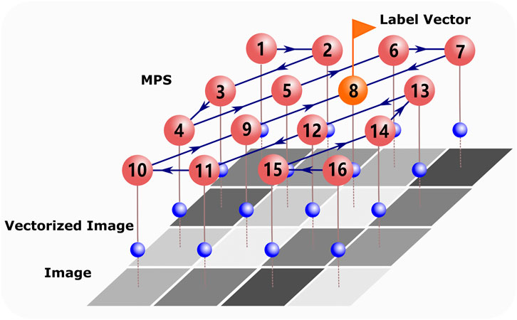
FIGURE 1. Illustration of MPS $\hat{\mathbf{\Psi }}$ for image classification. The pixels in an image are vectorized to many-qubit states v by the feature map (Eq. 1), and then be contracted with the MPS $\hat{\mathbf{\Psi }}$ to obtain the prediction of the classification (Eq. 3). The MPS illustrated here covers the 2D image in a zig-zag path. Each red or orange ball represents a tensor A^[l], and the number l on the tensors indicates tensors’ ordering in the MPS. The tensor which is being optimized and carries the label bond is highlighted in orange color. $\hat{\mathbf{\Psi }}$ satisfies the orthogonal conditions indicated by the arrows.

2 Matrix Product State and Training Algorithm

2.1 Mapping Image to Quantum Space

TN machine learning contains two key ingredients. The first one is the feature map [33], which encodes each sample (image) to a multi-qubits product state. Following the conventional TN machine learning [28, 30], each feature (say p_n,l, the lth pixel of the nth image) is transformed to a single-site state given by a d-dimensional normalized vector w^[n,l] as

$w_m^{[n,l]}=\sqrt{\left(\genfrac{}{}{0.0pt}{}{d-1}{m-1}\right)}{\left[\cos \left(\frac{\theta \pi }{2}{p}_{n,l}\right)\right]}^{d-m}{\left[\sin \left(\frac{\theta \pi }{2}{p}_{n,l}\right)\right]}^{m-1},(1)$

where m runs from 1 to d, and θ is a hyper-parameter that controls the maximum angle. We take d = 2 in this work so each qubit state is ${\mathbf{w}}^{[n,l]}=w_1^{[n,l]}\left|\uparrow \right.⟩+w_2^{[n,l]}\left|\downarrow \right.⟩$. By adjusting θ in Eq. 1 as a hyper parameter, we find that the best accuracy is achieved for θ = 0.5 without the discrete cosine transformation (DCT) [75–77] and for θ = 7.8 with DCT. These values are used in the following numerical experiments (see Supplementary Appendix B for a discussion on θ). Note that here we use the bold symbols to represent tensors without writing the components explicitly. In this way, the nth image that contains L pixels is mapped to a L-qubit product state

${\mathbf{v}}^{[n]}=\prod _{\otimes l=1}^L{\mathbf{w}}^{[n,l]}.(2)$

Besides mapping an image to a product state, there are other types of quantum image representation [78–81], for example, the FRQI [78] and 2-D QSNA [79] where the image is encoded in an entangled state to minimize the needed number of qubits. Here we choose the product state representation to cater for the MPS structure.

2.2 Matrix Product State Representation and Training Algorithm

The second key ingredient concerns the MPS representation and the training algorithm. TN provides a powerful mathematical tool to represent the wavefunction as a network of connected tensors. In the context of quantum many-body physics, TN has been widely used, for example, to simulate the ground states, the dynamic properties, and the finite temperature properties of quantum lattice models [43–45, 55, 56, 82–90]. For the image classification of ten digits, we expect the short-range correlation between pixels, which makes using MPS feasible [30]. An evidence for the short-range correlation among pixels is the superior performance of convolutional neural network with small convolution kernels. One may expect the MPS representation to be less efficient when working with images with long-range correlation (one example may be the images with fractal patterns).

In our TN machine learning setup, a D-class classifier is a linear map $\hat{\mathbf{\Psi }}$ which maps a d^L-dimensional vector v^[n] to a D-dimensional vector u^[n], with D being the number of image classes in the classification. Its components are ${\hat{\mathrm{\Psi }}}_{b,s_1\cdots s_L}$, where the index b is the D-dimensional label bond, and the indexes {s_l} are the physical bonds (which will be contracted with the vectorized images {v^[n]}). The prediction of the classification for the nth image is obtained by contracting the corresponding vectors v^[n] (in Eq. 2) with $\hat{\mathbf{\Psi }}$ as

$u_b^{[n]}=\sum _{s_1\cdots s_L}{\hat{\mathrm{\Psi }}}_{b,s_1\cdots s_L}{\mathbf{v}}_{s_1\cdots s_L}^{[n]}.(3)$

The bth component $u_b^{[n]}$ of u^[n] gives the prediction of the probability for the nth image being in the bth class.

$\hat{\mathbf{\Psi }}$ suffers an exponentially scaled parameter complexity as L grows. To represent $\hat{\mathbf{\Psi }}$ efficiently, we take the MPS ansatz (Figure 1). MPS is one of the simplest 1D TN structure, which is convenient and efficient [28, 29]. The specific form of MPS we use is

$\begin{array}{cc}\hfill & {\hat{\mathrm{\Psi }}}_{b,s_1\cdots s_L}=\hfill \\ \hfill & \sum _{a_1\cdots a_{L-1}}{A}_{s_1,a_1}^{[1]}{A}_{s_2,a_1,a_2}^{[2]}\cdots A_{s_l,b,a_{l-1},a_l}^{[l]}\cdots A_{s_L,a_{L-1}}^{[L]}.\hfill \end{array}(4)$

The elements of each tensor {A^[l]} are initialized as random numbers generated from the normal distribution N (0, 1). The indexes {a}, which are called the virtual bonds, will be summed over. The dimension χ of the virtual bonds determines the maximal entanglement that can be carried by the MPS. With the MPS ansatz, the total number of parameters in $\hat{\mathbf{\Psi }}$ increases only linearly with L, i.e., O (dχ²L). We take χ = 32 for the numerical simulations in this work.

To train the MPS $\hat{\mathbf{\Psi }}$, we optimize the tensors {A^[l]} one by one to minimize the cost function–the negative logarithmic likelihood (NLL) [29, 91].

$C=-\frac{1}{|\mathrm{\Gamma }|}\sum _{n\in \mathrm{\Gamma }}\ln \frac{|u_{b_n}^{[n]}{|}^2}{Z}.(5)$

For supervised learning task, b_n in the $u_{b_n}^{[n]}$ denotes the known correct classification of the nth image in the training set. The predicted probability of the nth image being correctly classified as the b_n-th class is given by $\frac{|u_{b_n}^{[n]}{|}^2}{Z}$ with Z the norm of the MPS. In the practical simulation, we utilize the canonical form of MPS [29] and keep Z = 1 in the whole updating process. Γ denotes the total number of the training samples, and the summation goes through the training set. There is no upper bound for the cost function and the lower bound is 0 when the predictions of all training samples perfectly have $u_b^{[n]}=1$ for b = b_n and $u_b^{[n]}=0$ for b ≠ b_n.

We use the gradient descent algorithm [28] to optimize {A^[l]} one by one, sweeping back and forth along the MPS until the cost function converges. The label b is always at the tensor that we wish to optimize. Let’s take update forward as an example, to update $A_{s_{l}b{a}_{l-1}{a}_l}^{[l]}$, we first decompose it using singular value decomposition (SVD):

$A_{s_{l}b{a}_{l-1}{a}_l}^{[l]}=\sum _{a_l{a}_{l^{\prime }}}{U}_{a_{l-1}{s}_l,a_l}{S}_{a_l,a_{l^{\prime }}}{V}_{a_{l^{\prime }},a_{l}b}.(6)$

We then replace A^[l] with U and A^[l+1] with SVA^[l+1]. Notice that the label b is passed to A^[l+1] in this step. After that, we perform the gradient descent algorithm and A^[l] is updated by A^[l] − α∂C/∂A^[l] with other tensors being fixed. The step of the gradient descent (learning rate) is controlled by α, which is a small empirical parameter. Having updated A^[l], we proceed forward to update A^[l+1] using the same method and pass the label b to A^[l+2], so on and so forth. After a round of optimization, all the tensors are updated once, and the label b is back on the tensor we start at.

2.3 Entanglement of Matrix Product State

In quantum information science, entanglement measures the quantum version of correlation that characterizes how two subsystems are correlated. The MPS classifier can be regarded as a many-qubit quantum state. Given a trained classifier $\hat{\mathbf{\Psi }}$, to capture its entanglement, we introduce two entanglement measures: single-site entanglement entropy (SEE) and bipartite entanglement entropy (BEE). The reduced density matrix ${\hat{\mathit{\rho }}}^{[l]}$ of the lth site is obtained by contracting all indexes except s_l and s_l′,

${\hat{\rho }}_{s_l{s\prime }_l^{}}^{[l]}=\sum _{b,s_1\cdots s_{l-1}{s}_{l+1}\cdots s_L}{\hat{\mathrm{\Psi }}}_{b,s_1\cdots s_l\cdots s_L}{\hat{\mathrm{\Psi }}}_{b,s_1\cdots s_l^{\prime }\cdots s_L}.(7)$

Note ${\hat{\mathit{\rho }}}^{[l]}$ is non-negative. When calculating ${\hat{\mathit{\rho }}}^{[l]}$ with an MPS, the leading computational complexity scales linearly with the length of the MPS (O(L)). After normalizing ${\hat{\mathit{\rho }}}^{[l]}$ by ${\hat{\mathit{\rho }}}^{[l]}\leftarrow {\hat{\mathit{\rho }}}^{[l]}/\text{Tr}{\hat{\mathit{\rho }}}^{[l]}$, the SEE can be defined as

$S_{\text{SEE}}^{[l]}=-\text{Tr}{\hat{\mathit{\rho }}}^{[l]}\ln {\hat{\mathit{\rho }}}^{[l]}.(8)$

SEE captures the entanglement entropy between one qubit located at site l and the rest of the system.

The BEE is defined as the entanglement entropy between the first l qubits of the MPS and the rest, which can be obtained by the reduced density matrix after tracing over the first l sites of the MPS. Another way to compute BEE is by implementing SVD, where BEE is calculated from the singular values (Schmidt numbers). By grouping the indexes b, s₁⋯s_l and s_l+1⋯s_L, we obtain the following SVD decomposition on the virtual bond:

${\hat{\mathrm{\Psi }}}_{b,s_1\cdots s_l{s}_{l+1}\cdots s_L}=\sum _{\alpha {\alpha }^{\prime }}{X}_{b,s_1\cdots s_l,\alpha }{\lambda }_{\alpha {\alpha }^{\prime }}^{[l]}{Y}_{{\alpha }^{\prime },s_{l+1}\cdots s_L},(9)$

where the singular values are given by the positive-definite diagonal matrix λ^[l], and X and Y satisfy the orthogonal conditions XX^T = Y^TY = I. Normalizing λ^[l] by λ^[l] ←λ^[l]/Tr λ^[l], BEE can be expressed as

$S_{\text{BEE}}^{[l]}=-\sum _{\alpha }{({\lambda }_{\alpha \alpha }^{[l]})}^2\ln {({\lambda }_{\alpha \alpha }^{[l]})}^2.(10)$

In the context of MPS, one can implement the gauge transformations to bring the MPS to the center-orthogonal form [47]. The details of the central-orthogonal form of the MPS classifier for supervised machine learning can be found in Ref. [28]. Under the center-orthogonal form, λ^[l] can be obtained by the SVD of the tensor in the center A^[l] as $A_{s_l{a}_{l-1}{a}_l}^{[l]}={\sum }_{\alpha {\alpha }^{\prime }}{X}_{s_l{a}_{l-1},\alpha }{\lambda }_{\alpha {\alpha }^{\prime }}^{[l]}{Y}_{{\alpha }^{\prime },a_l}$. The leading computational cost (of the center-orthogonalization and SVD) scales linearly with the MPS size (O(L)).

It is worthy to notice that SVD is also widely used in the classical image processing algorithms [92–94], where the singular values are the global properties of the images. In our algorithm, the SVD is performed on the virtual bond connecting different sites. In this way, the singular values for a given cut reflect the local properties (importance of features), which makes it different from the classical case.

3 Feature Extraction Based on Entanglement

3.1 Entanglement in Image Classification

Taking the “1-7” binary classifier as an example, the entanglement properties of the MPS classifier are shown in Figure 2 (we include more data on binary classifiers in Supplementary Appendix D). The size and darkness of the nodes illustrate the strength of the SEE of each site, and the thickness of the bonds shows the strength of the BEE obtained by cutting the MPS into two pieces at the bonds. An important part of our proposal is the way of arranging the features in a 1D path to contract with the MPS. For the images, the features (pixels) are originally placed as a 2D array, while the tensors in an MPS are connected as a 1D network. Therefore, a 1D path should be chosen so that each feature (after implementing the feature map) is contracted with one of the tensors in the MPS. Figure 2 illustrates three different paths we use in this work.

FIGURE 2

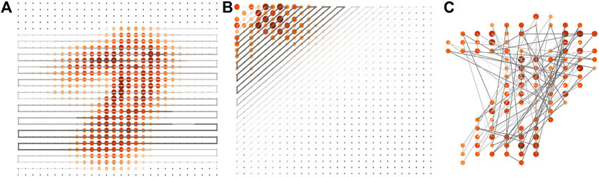
FIGURE 2. The entanglement properties of the “1–7” binary MPS classifier using different paths (which show how the MPS covers the 2D images). The size and darkness of nodes represent the SEE’s strength on each site (sites with vanishing SEE are represented by small black dots). The thickness of the bonds represents the strength of the BEE by cutting the MPS at the bonds. (A) demonstrates the SEE and BEE of the MPS trained by images (without DCT). In this case, we use the “line-by-line” path, and the label is at the middle site. (B) shows the SEE and BEE of the MPS trained by the frequency components after the DCT, where we use the “zig-zag” path. In this case, we put the label on the first tensor of the MPS. (C) gives the results trained by images (without DCT) using an optimized path where the sites with larger SEE are arranged closer to the center of the MPS. We only keep the 100 pixels with the largest SEE, and the label is put on the middle site of the MPS.

Figure 2A shows a 1D path that connects the neighboring rows in 2D in a head-to-tail manner, which we dub as the “line-by-line” path. Note the label is put in the middle of the MPS. By naked eyes, one can see that the SEE forms a shape of overlapped “1” and “7”. This implies that the sites with larger SEE generally form the shape of the digits to be classified. Meanwhile, the sites close to the edge of the image exhibit almost vanishing SEE. Besides, by following the 1D path, the BEE increases when going from either end of the MPS to the middle. These observations are consistent with the fact that the pixels near the edges of the images contain almost no information. Our results suggest that the importance of features can be characterized by the entanglement properties.

In Figure 2B, we first transform the images to the frequency components using discrete cosine transformation (DCT) [75–77], which is a “real-number” version of the Fourier transformation (see more details of DCT in Supplementary Appendix C). The frequency components are the coefficients of the image’s frequency modes in the horizontal and vertical directions. The frequency increases when going from the left-top to the right-bottom corner of the 2D array. This allows a natural choice of the 1D path from left-top to the right-bottom (Figure 2B), which we call the “zig-zag” path. In this case, the label bond is put on the first tensor of the MPS. The frequency components are then mapped to vectors by the feature map and subsequently contracted with the MPS to predict the classification.

We still take the “1–7” binary classifier as an example to investigate the SEE and BEE of the MPS. The sites with larger SEE appear mainly at the left-top corner, which shows that the relatively highly entangled qubits correspond to the low-frequency components. This agrees with the well-known knowledge in computer vision that the main information for images is usually encoded in the low-frequency data. It further verifies our claim that the importance of features can be characterized by the entanglement properties. Compared to the “line-by-line” path, the number of the highly entangled sites is much less than that in Figure 2A, which shows that images will become much sparser after DCT.

Fig. 2 (c) c MPS, where the real-space pixels are arranged in such a way that those with larger SEE are closer to the center of the MPS (the label is at the center). Only 100 features that possess the largest SEE are retained, and the rest are discarded. In the following, we will propose a feature extraction scheme by using such an optimized path.

3.2 Feature Extraction Based on Entanglement

If the lth qubit in the MPS gives zero SEE, it means there is no entanglement between this qubit and the other qubits (including the label). In this case, the classification will not be affected no matter how the value of the lth feature changes. In other words, the features corresponding to the qubits with vanishing SEE are irrelevant to the prediction of the classification.

Based on this observation, we propose the following feature extraction algorithm, which extract the important features from the samples according to the entanglement properties of the MPS. With a MPS trained by minimizing the cost function (Eq. 5), we first optimize the path of the MPS according to SEE so that the important features (with larger SEE) are arranged in the middle, closer to the label index (Figure 2C). Using the optimized path, we then re-initialized and train a new MPS, whose SEE would become more concentrated when going from the middle to the ends. We use the new SEE for the next path optimization. This process is repeated until SEE is sufficiently concentrated. We then calculate the BEE and keep only $\tilde{L}$ features with the largest BEE in the middle of MPS in the optimized path (Figure 3). Finally, we can train the MPS classifier using only the retained features. The main steps of our algorithm are listed in Figure 4.

FIGURE 3

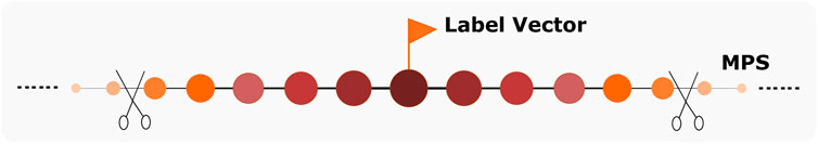
FIGURE 3. Illustration of the feature extraction by cutting the “tails” of the MPS. The size and darkness of nodes represent SEE’s strength at each site, and the thickness of bonds represent the BEE’s strength by cutting the MPS at the bonds. After optimizing the path based on the SEE, the MPS is cut and only $\tilde{L}$ features with largest BEE are retained. The qubits on the cut tails possess small entanglement with the bulk of the MPS, which can be safely discarded.

FIGURE 4

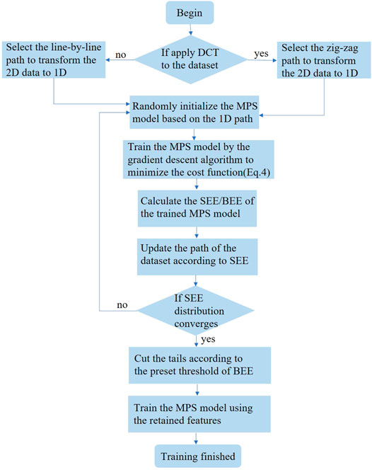
FIGURE 4. The flowchart of the feature extraction algorithm.

To explain how this algorithm works, let us give a simple example with a three-qubit quantum state |ψ⟩ = |↑↑↓⟩ + |↓↑↑⟩, where |↑⟩ and |↓⟩ stand for the spin-up and spin-down states, respectively. We assume that the first spin carries the label information of a binary classification. Since the second spin of |ψ⟩ can be factored out as a direct product, ${\hat{\mathit{\rho }}}^{[2]}$ is a pure state, and the SEE of the second spin is zero. Therefore, discarding the feature corresponding to the second spin will not affect the classification.

Meanwhile, path optimization will lead to a more efficient MPS representation of the classifier. By writing the wave function into a three-site MPS, one can check that the two virtual bonds are both two-dimensional. The total number of parameters of this MPS is 2² + 2³ + 2² = 16. However, if we define the MPS after moving the second qubit to either end of the chain (say swapping it with the third qubit), the wave function becomes |ψ⟩ = |↑↓↑⟩ + |↓↑↑⟩ = (|↑↓⟩ + |↓↑⟩) ⊗|↑⟩. Now the virtual bonds of the MPS are two- and one-dimensional respectively, and the total number of parameters is reduced to 2² + 2² + 2 = 10.

We test the feature extraction algorithm in the ten-class MPS classifier of the images in the MNIST dataset. We randomly selected one thousand images from each class as the training set. Figure 5A shows the SEE of the trained MPS (trained by images without DCT) with and without optimizing the path according to SEE. Without path optimization, the features with large SEE are distributed almost over the whole MPS; while using path optimization, the larger values of the SEE are much more concentrated to the middle. Note we optimize the path according to the SEE of the previously trained MPS, and then we train a new MPS with the updated path, whose SEE would decrease in general but fluctuate when going from the middle to the ends. The magnitude of the fluctuations converges after optimizing the path for O (1) times, and the features with large SEE will be well concentrated to the middle. Figure 5B shows the SEE of the MPS trained by the frequency components of the images (after DCT) with and without the path optimization. The number of features with large SEE becomes much smaller than that from the MPS trained without DCT. This indicates we can achieve a similar accuracy with much less features when using DCT.

FIGURE 5

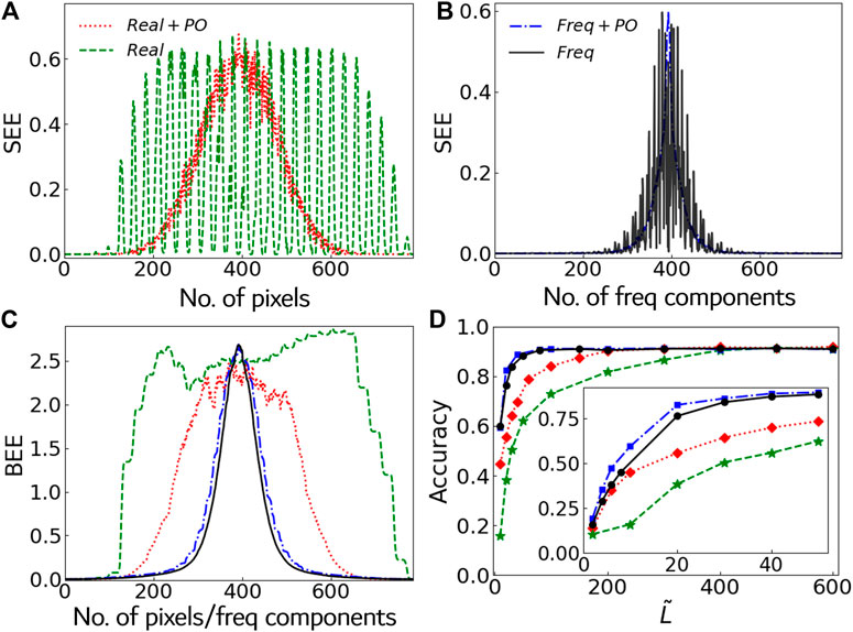
FIGURE 5. (A) and (B) show the SEE of the ten-class MPS classifier (i.e., D = 10) with or without DCT/path optimization. (C) shows the BEE of these four cases. (D) demonstrates the classification accuracy on the test dataset versus the number of the retained extracted features $\tilde{L}$.

Figure 5C shows the BEE of the MPS’s. It can be seen that the tails with small BEE become longer by either implementing DCT or optimizing the path, which implies that more features can be discarded safely. Figure 5D shows the ten-class classification accuracy for the test set where $\tilde{L}$ is the number of retained features. We observe that the testing accuracies in the four cases are almost identical as long as we keep sufficient features ($\tilde{L}>400$ approximately). With relatively small numbers of the extracted features, higher accuracy can be achieved using DCT or path optimization. For instance, with only 20 features, the accuracy is 82% by using DCT and the optimized path, while the accuracy is 56 and 76% with only the path optimization and DCT, respectively (Figure 5D). When keeping $\tilde{L}=L/10$, the decrease of accuracy is only O (10^–3) by using DCT and path optimization.

We also apply our feature extraction algorithm to the binary MPS classifiers of the images in Fashion-MNIST dataset [95] (see Supplementary Appendix E for details), where we come to the similar observations. This show the algorithm is universal and capable of handling the more complicated dataset.

4 Summary

In this work, we implement numerical experiments with MPS for image classification and explicitly show how entanglement properties of MPS can be used to characterize the importance of features. A novel entanglement-based feature extraction algorithm is proposed by discarding the features that correspond to the less entangled qubits of the MPS. We test our proposal on the MNIST dataset of handwritten digits and show that high accuracy can be achieved with a small number of retained features using DCT and path optimization. Our results show that for the ten-class classifiers of the MNIST dataset, the number of features can be safely lowered to less than 1/10 of the original number.

In the literature, the feature extraction of images is typically achieved by image segmentation and matrix transformation (applying various filters) [96–99]. The spatial or transformed features are directly used as reference to decide which features are more important. Our algorithm does not rely on the segmentation, and focus on the correlation between features.

Our work gives a convincing startup of building connections between the entanglement properties (SEE/BEE of the MPS) and machine learning tasks. Interpretability is a challenging issue in machine learning [66–73], which concerns the interpretations of how machine learning models work, how to design the models, how information flows during the processing, and so on. One important issue of interpretability is to characterize the importance of features, which will assist in explaining the main factors that affect the results and implementing feature extractions, to name but a few. In the literature, some methods are proposed to improve the intepretability of machine learning [100–105], although there still exist various limitations. Our work explicitly shows how entanglement properties of MPS can be used to characterize the importance of features. Therefore, our work can be regarded as a tensor network version of sensitivity analysis [106], which may provide an alternative to other interpretability methods, such as the influence functions and Kernel method, etc. Our proposal can also be applied to the TN’s with more sophisticated architecture, such as projected entangled pair states [43, 57, 107], for efficient machine learning.

Data Availability Statement

The original contributions presented in the study are included in the article/Supplementary Material, further inquiries can be directed to the corresponding authors.

Author Contributions

All of the authors contributed in designing the work, analyzing the results, writing and revising the manuscript. The numerical simulation were done by YL and W-JL with equal contribution.

Funding

This work was supported by ERC AdG OSYRIS (ERC-2013-AdG Grant No. 339106), Spanish Ministry MINECO (National Plan 15 Grant: FISICATEAMO No. FIS2016-79508-P, SEVERO OCHOA No. SEV-2015–0522), Generalitat de Catalunya (AGAUR Grant No. 2017 SGR 1341 and CERCA/Program), Fundació Privada Cellex, EU FETPRO QUIC (H2020-FETPROACT-2014 No. 641122), the National Science Centre, and Poland-Symfonia Grant No. 2016/20/W/ST4/00314. S-JR was supported by Fundació Catalunya - La Pedrera. Ignacio Cirac Program Chair and is supported by Beijing Natural Science Foundation (Grant No. 1192005 and No. Z180013), Foundation of Beijing Education Committees (Grant No. KM202010028013), and the Academy for Multidisciplinary Studies, Capital Normal University. XZ is supported by the National Natural Science Foundation of China (No. 11404413), the Natural Science Foundation of Guangdong Province (No. 2015A030313188), and the Guangdong Science and Technology Innovation Youth Talent Program (Grant No. 2016TQ03X688). ML acknowledges the support by Capital Normal University on academic visiting. W-JL and GS are supported by in part by the NSFC (Grant No. 11834014), the National Key R&D Program of China (Grant No. 2018FYA0305804), the Strategetic Priority Research Program of the Chinese Academy of Sciences (Grant No. XDB28000000), and Beijing Municipal Science and Technology Commission (Grant No. Z190011).

Conflict of Interest

The authors declare that the research was conducted in the absence of any commercial or financial relationships that could be construed as a potential conflict of interest.

Publisher’s Note

All claims expressed in this article are solely those of the authors and do not necessarily represent those of their affiliated organizations, or those of the publisher, the editors and the reviewers. Any product that may be evaluated in this article, or claim that may be made by its manufacturer, is not guaranteed or endorsed by the publisher.

Acknowledgments

S-JR thanks Anna Dawid Lekowska, Lei Wang, Ding Liu, Cheng Peng, Zheng-Zhi Sun, Ivan Glasser, and Peter Wittek for stimulating discussions. YL thanks Naichao Hu for helpful suggestions of writing the manuscript.

Supplementary Material

The Supplementary Material for this article can be found online at: https://www.frontiersin.org/articles/10.3389/fams.2021.716044/full#supplementary-material

References

1. Lewenstein, M. Quantum Perceptrons. J Mod Opt (1994) 41:2491–501. doi:10.1080/09500349414552331

CrossRef Full Text | Google Scholar

2. Chrisley, R. New Directions in Cognitive Science. In Proceedings of the International Symposium, Saariselka 4-9 (1995).

Google Scholar

3. Kak, SC. Quantum Neural Computing. Adv Imaging Electron Phys (1995) 94:259–313. doi:10.1016/s1076-5670(08)70147-2

CrossRef Full Text | Google Scholar

4. Schuld, M, Sinayskiy, I, and Petruccione, F. The Quest for a Quantum Neural Network. Quan Inf Process (2014) 13:2567–86. doi:10.1007/s11128-014-0809-8

CrossRef Full Text | Google Scholar

5. Baaquie, BE. Quantum Finance: Path Integrals and Hamiltonians for Options and Interest Rates. Cambridge University Press (2007). Journal of Modern Optics.

Google Scholar

6. Eisert, J, Wilkens, M, and Lewenstein, M. Quantum Games and Quantum Strategies. Phys Rev Lett (1999) 83:3077–80. doi:10.1103/physrevlett.83.3077

CrossRef Full Text | Google Scholar

7. Johnson, NF. Enhancons, Fuzzy spheres and Multimonopoles. Phys Rev A (2001) 63(R):020302. doi:10.1103/physrevd.63.065004

CrossRef Full Text

8. Du, J, Li, H, Xu, X, Shi, M, Wu, J, Zhou, X, et al. Experimental Realization of Quantum Games on a Quantum Computer. Phys Rev Lett (2002) 88:137902. doi:10.1103/physrevlett.88.137902

PubMed Abstract | CrossRef Full Text | Google Scholar

9. Dunjko, V, Taylor, JM, and Briegel, HJ. Quantum-Enhanced Machine Learning. Phys Rev Lett (2016) 117:130501. doi:10.1103/physrevlett.117.130501

PubMed Abstract | CrossRef Full Text | Google Scholar

10. Dunjko, V, Liu, YK, Wu, X, and Taylor, JM. Exponential improvements for quantum-accessible reinforcement learning. arXiv:1710.11160.

11. Lucas, L. Basic protocols in quantum reinforcement learning with superconducting circuits. Scientific Rep (2017) 7:1–10.

12. Monràs, A, Sentís, G, and Wittek, P. Inductive Supervised Quantum Learning. Phys Rev Lett (2017) 118:190503. doi:10.1103/physrevlett.118.190503

PubMed Abstract | CrossRef Full Text | Google Scholar

13. Hallam, A, Grant, E, Stojevic, V, Severini, S, and Green, AG. Compact Neural Networks based on the Multiscale Entanglement Renormalization Ansatz. British Machine Vision Conference 2018, {BMVC} 2018, Newcastle, UK, September 3-6, 2018 (2018).

14. Liu, J-G, and Wang, L. Differentiable Learning of Quantum Circuit Born Machines. Phys Rev A (2018) 98:062324. doi:10.1103/physreva.98.062324

CrossRef Full Text | Google Scholar

15. Hao, B-L, Lee, HC, and Zhang, S-Y. Fractals Related to Long DNA Sequences and Complete Genomes. Chaos, Solitons & Fractals (2000) 11:825–36. doi:10.1016/s0960-0779(98)00182-9

CrossRef Full Text | Google Scholar

16. Latorre, JI. Image compression and entanglement. arXiv: quant-ph/0510031.

17. Le, PQ, Dong, F, and Hirota, K. A Flexible Representation of Quantum Images for Polynomial Preparation, Image Compression, and Processing Operations. Quan Inf. Process (2011) 10:63–84. doi:10.1007/s11128-010-0177-y

CrossRef Full Text | Google Scholar

18. Rodríguez-Laguna, J, Migdał, P, Berganza, MI, Lewenstein, M, and Sierra, G. Qubism: Self-Similar Visualization of Many-Body Wavefunctions. New J Phys (2012) 14:053028. doi:10.1088/1367-2630/14/5/053028

CrossRef Full Text | Google Scholar

19. O’brien, JL, Furusawa, A, and Vučković, J. Photonic quantum technologies. Nat Photon (2009) 3:687.

CrossRef Full Text

20. Mohseni, M, Read, P, Neven, H, Boixo, S, Denchev, V, Babbush, R, et al. Commercialize Quantum Technologies in Five Years. Nature (2017) 543:171–4. doi:10.1038/543171a

PubMed Abstract | CrossRef Full Text | Google Scholar

21. Dowling, JP, and Milburn, GJ. Quantum Technology: the Second Quantum Revolution. Philos Trans R Soc Lond Ser A: Math Phys Eng Sci (2003) 361:1655–74. doi:10.1098/rsta.2003.1227

CrossRef Full Text | Google Scholar

22. Deutsch, D. Physics, philosophy and quantum technology. Proceedings of the Sixth International Conference on Quantum Communication, Measurement and Computing. Princeton, NJ: Rinton Press (2003). p. 419–26.

23. Huggins, W, Patil, P, Mitchell, B, Whaley, KB, and Stoudenmire, EM. Towards Quantum Machine Learning with Tensor Networks. Quan Sci. Technol. (2019) 4:024001. doi:10.1088/2058-9565/aaea94

CrossRef Full Text | Google Scholar

24. Cai, X-D, Wu, D, Su, Z-E, Chen, M-C, Wang, X-L, Li, L, et al. Entanglement-Based Machine Learning on a Quantum Computer. Phys Rev Lett (2015) 114:110504. doi:10.1103/physrevlett.114.110504

PubMed Abstract | CrossRef Full Text | Google Scholar

25. Lloyd, S, Mohseni, M, and Rebentrost, P. Quantum algorithms for supervised and unsupervised machine learning (2013). arXiv:1307.0411.

26. Lamata, L. Basic Protocols in Quantum Reinforcement Learning with Superconducting Circuits. Sci Rep (2017) 7:1609. doi:10.1038/s41598-017-01711-6

PubMed Abstract | CrossRef Full Text | Google Scholar

27. Biamonte, J, Wittek, P, Pancotti, N, Rebentrost, P, Wiebe, N, and Lloyd, S. Quantum Machine Learning. Nature (2017) 549:195–202. doi:10.1038/nature23474

PubMed Abstract | CrossRef Full Text | Google Scholar

28. Stoudenmire, E, and Schwab, DJ. Supervised Learning with Tensor Networks. Advances in Neural Information Processing Systems (2016). Curran Associates, Inc. 4799–807.

29. Han, Z-Y, Wang, J, Fan, H, Wang, L, and Zhang, P. Phys Rev X (2018) 8:031012. doi:10.1103/physrevx.8.031012

CrossRef Full Text

30. Martyn, J, Vidal, G, Roberts, C, and Leichenauer, S. Entanglement and tensor networks for supervised image classification (2020). arXiv:2007.06082.

31. Pestun, V, and Vlassopoulos, Y. Tensor network language model (2017). arXiv:1710.10248.

32. Liu, D, Ran, S-J, Wittek, P, Peng, C, García, RB, Su, G, et al. Machine Learning by Unitary Tensor Network of Hierarchical Tree Structure. New J Phys (2019) 21:073059. doi:10.1088/1367-2630/ab31ef

CrossRef Full Text | Google Scholar

33. Stoudenmire, EM. Learning Relevant Features of Data with Multi-Scale Tensor Networks. Quan Sci. Technol. (2018) 3:034003. doi:10.1088/2058-9565/aaba1a

CrossRef Full Text | Google Scholar

34. Levine, Y, Yakira, D, Cohen, N, and Shashua, A. Deep Learning and Quantum Entanglement: Fundamental Connections with Implications to Network Design. International Conference on Learning Representations (2017) 01552.

35. Glasser, I, Pancotti, N, and Cirac, JI. From Probabilistic Graphical Models to Generalized Tensor Networks for Supervised Learning. IEEE Access (2020) 8:68169–82. doi:10.1109/access.2020.2986279

CrossRef Full Text | Google Scholar

36. Selvan, R, and Dam, EB. Tensor networks for medical image classification Medical Imaging with Deep Learning (2020) 721–732.

37. Trenti, M, Sestini, L, Gianelle, A, Zuliani, D, Felser, T, and Lucchesi, D. Quantum-inspired Machine Learning on high-energy physics data (2020). arXiv:2004.13747.

38. Efthymiou, S, Hidary, J, and Leichenauer, S. Tensornetwork for machine learning (2019). arXiv:1906.06329.

39. Wang, J, Roberts, C, Vidal, G, and Leichenauer, S. Anomaly detection with tensor networks (2020). arXiv:2006.02516.

40. Cheng, S, Wang, L, Xiang, T, and Zhang, P. Tree Tensor Networks for Generative Modeling. Phys Rev B (2019) 99:155131. doi:10.1103/physrevb.99.155131

CrossRef Full Text | Google Scholar

41. Reyes, J, and Stoudenmire, M. A multi-scale tensor network architecture for classification and regression (2020). arXiv:2001.08286.

42. Sun, Z-Z, Peng, C, Liu, D, Ran, SJ, and Su, G. Generative Tensor Network Classification Model for Supervised Machine Learning Phys Rev B (2020) 101:075135. doi:10.1103/physrevb.101.075135

CrossRef Full Text | Google Scholar

43. Orús, R. A Practical Introduction to Tensor Networks: Matrix Product States and Projected Entangled Pair States. Ann Phys (2014) 349:117–58. doi:10.1016/j.aop.2014.06.013

CrossRef Full Text | Google Scholar

44. Cirac, JI, and Verstraete, F. Renormalization and Tensor Product States in Spin Chains and Lattices. J Phys A: Math Theor (2009) 42:504004. doi:10.1088/1751-8113/42/50/504004

CrossRef Full Text | Google Scholar

45. Bridgeman, JC, and Chubb, CT. Hand-waving and Interpretive Dance: an Introductory Course on Tensor Networks. J Phys A: Math Theor (2017) 50:223001. doi:10.1088/1751-8121/aa6dc3

CrossRef Full Text | Google Scholar

46. Orús, R. Advances on Tensor Network Theory: Symmetries, Fermions, Entanglement, and Holography. Eur Phys J B (2014) 87:280. doi:10.1140/epjb/e2014-50502-9

CrossRef Full Text | Google Scholar

47. Ran, SJ, Tirrito, E, Peng, C, Chen, X, Tagliacozzo, L, Su, G, et al. Tensor Network Contractions: Methods And Applications To Quantum Many-Body Systems, Lecture Notes in Physics. Cham: Springer (2020).

48. Verstraete, F, Wolf, MM, Perez-Garcia, D, and Cirac, JI. Criticality, the Area Law, and the Computational Power of Projected Entangled Pair States. Phys Rev Lett (2006) 96:220601. doi:10.1103/physrevlett.96.220601

PubMed Abstract | CrossRef Full Text | Google Scholar

49. Schuch, N, Poilblanc, D, Cirac, JI, and Pérez-García, D. Resonating Valence Bond States in the PEPS Formalism. Phys Rev B (2012) 86:115108. doi:10.1103/physrevb.86.115108

CrossRef Full Text | Google Scholar

50. Verstraete, F, and Cirac, JI. Phys Rev B (2006) 73:094423. doi:10.1103/physrevb.73.094423

CrossRef Full Text

51. Pérez-García, D, Verstraete, F, Wolf, MM, and Cirac, JI. Matrix Product State Representations. Qic (2007) 7:401–30. doi:10.26421/qic7.5-6-1

CrossRef Full Text | Google Scholar

52. White, SR. Density Matrix Formulation for Quantum Renormalization Groups. Phys Rev Lett (1992) 69:2863–6. doi:10.1103/physrevlett.69.2863

PubMed Abstract | CrossRef Full Text | Google Scholar

53. Fannes, M, Nachtergaele, B, and Werner, RF. Finitely Correlated States on Quantum Spin Chains. Commun.Math Phys (1992) 144:443–90. doi:10.1007/bf02099178

CrossRef Full Text | Google Scholar

54. Rommer, S, and Östlund, S. Class of Ansatz Wave Functions for One-Dimensional Spin Systems and Their Relation to the Density Matrix Renormalization Group. Phys Rev B (1997) 55:2164–81. doi:10.1103/physrevb.55.2164

CrossRef Full Text | Google Scholar

55. Vidal, G. Efficient Classical Simulation of Slightly Entangled Quantum Computations. Phys Rev Lett (2003) 91:147902. doi:10.1103/physrevlett.91.147902

PubMed Abstract | CrossRef Full Text | Google Scholar

56. Vidal, G. Efficient Simulation of One-Dimensional Quantum Many-Body Systems. Phys Rev Lett (2004) 93:040502. doi:10.1103/physrevlett.93.040502

PubMed Abstract | CrossRef Full Text | Google Scholar

57. Verstraete, F, and Cirac, JI. Renormalization algorithms for quantum-many body systems in two and higher dimensions (2004). arXiv:cond-mat/0407066.

58. Shi, YY, Duan, LM, and Vidal, G. Classical Simulation Of Quantum Many-Body Systems With a Tree Tensor Network. Phys Rev A (2006) 74:022320. doi:10.1103/physreva.74.022320

CrossRef Full Text | Google Scholar

59. Murg, V, Verstraete, F, Legeza, Ö, and Noack, RM. Simulating Strongly Correlated Quantum Systems with Tree Tensor Networks. Phys Rev B (2010) 82:205105. doi:10.1103/physrevb.82.205105

CrossRef Full Text | Google Scholar

60. Vidal, G. Entanglement Renormalization. Phys Rev Lett (2007) 99:220405. doi:10.1103/physrevlett.99.220405

PubMed Abstract | CrossRef Full Text | Google Scholar

61. Vidal, G. Class of Quantum Many-Body States that Can Be Efficiently Simulated. Phys Rev Lett (2008) 101:110501. doi:10.1103/physrevlett.101.110501

PubMed Abstract | CrossRef Full Text | Google Scholar

62. Evenbly, G, and Vidal, G. Algorithms for Entanglement Renormalization. Phys Rev B (2009) 79:144108. doi:10.1103/physrevb.79.144108

CrossRef Full Text | Google Scholar

63. Liu, J-G, Zhang, Y-H, Yuan, W, and Lei, W. Variational Quantum Eigensolver With Fewer Qubits. Phys Rev Res (2019) 1:2. doi:10.1103/physrevresearch.1.023025

CrossRef Full Text | Google Scholar

64. Eichler, C, Mlynek, J, Butscher, J, Kurpiers, P, Hammerer, K, Osborne, TJ, et al. Exploring Interacting Quantum Many-Body Systems By Experimentally Creating Continuous Matrix Product States in Superconducting Circuits. Phys Rev X (2015) 5:4. doi:10.1103/physrevx.5.041044

CrossRef Full Text | Google Scholar

65. Grant, E, Benedetti, M, Cao, S, Hallam, A, Lockhart, J, Stojevic, V, et al. Hierarchical Quantum Classifiers. Npj Quan Inf (2018) 4:65. doi:10.1038/s41534-018-0116-9

CrossRef Full Text | Google Scholar

66. Baehrens, A, Schroeter, T, and Harmeling, S. How to explain individual classification decisions. J Mach Learn Res (2010) 11:1803.

67. Selvaraju, RR, Cogswell, M, Das, A, Vedantam, R, Parikh, D, and Batra, D. Grad-CAM: Visual Explanations from Deep Networks via Gradient-Based Localization. Int J Comput Vis (2020) 128:336–59. doi:10.1007/s11263-019-01228-7

CrossRef Full Text | Google Scholar

68. Chattopadhyay, A, Sarkar, A, Howlader, P, and Balasubramanian, VN. Grad-CAM++: Generalized Gradient-Based Visual Explanations for Deep Convolutional Networks. 2018 IEEE Winter Conference on Applications of Computer Vision (WACV) (2018) 839–847.

69. Guidotti, R, Monreale, A, Ruggieri, S, Turini, F, Giannotti, F, and Pedreschi, D. A Survey of Methods for Explaining Black Box Models. ACM Comput Surv (2019) 51(5):1–42. doi:10.1145/3236009

CrossRef Full Text | Google Scholar

70. Zhang, Q, and Zhu, S-C. Visual interpretability for deep learning: a survey. Front Inform Technol Electron Eng (2018) 19:27–39. doi:10.1631/FITEE.1700808

71. Doshi-Velez, F, and Kim, B. Towards a rigorous science of interpretable machine learning. arXiv:1702.08608.

72. Cook, RD. Detection of Influential Observation in Linear Regression. Technometrics (1977) 19:15. doi:10.2307/1268249

CrossRef Full Text | Google Scholar

73. Anna, D, Huembeli, P, MichałTomza, ML, and Dauphin, A. Phase detection with neural networks: interpreting the black box. New J Phys (2020) 22:115001. doi:10.1088/1367-2630/abc463

CrossRef Full Text

74.Website of MNIST Dataset: http://yann.lecun.com/exdb/mnist/ (Accessed July 28, 2021).

75. Ahmed, N, Natarajan, T, and Rao, KR. Discrete Cosine Transform. IEEE Trans Comput (1974) C-23:90–3. doi:10.1109/t-c.1974.223784

CrossRef Full Text | Google Scholar

76. Holub, V, and Fridrich, J. Low-Complexity Features for JPEG Steganalysis Using Undecimated DCT. IEEE Trans.Inform.Forensic Secur. (2015) 10(2):219–28. doi:10.1109/tifs.2014.2364918

CrossRef Full Text | Google Scholar

77. Saad, MA, Bovik, AC, and Charrier, C. Blind Image Quality Assessment: A Natural Scene Statistics Approach in the DCT Domain. IEEE Trans Image Process (2012) 21:3339–52. doi:10.1109/tip.2012.2191563

PubMed Abstract | CrossRef Full Text | Google Scholar

78. Le, PQ, Iliyasu, AM, Dong, F, and Hirota, K. Berlin, Heidelberg: Springer (2011).

79. Srivastava, M, Roy-Moulick, S, and Panigrahi, PK. arxiv:1305.2251v4[cs.MM].

80. Yan, F, Iliyasu, AM, and Venegas-Andraca, SE. A Survey of Quantum Image Representations. Quan Inf Process (2016) 15(1):1–35. doi:10.1007/s11128-015-1195-6

CrossRef Full Text | Google Scholar

81. Su, J, Guo, X, Liu, C, and Li, L. A New Trend of Quantum Image Representations. IEEE Access (2020) 8:214520–37. doi:10.1109/access.2020.3039996

CrossRef Full Text | Google Scholar

82. Czarnik, P, Cincio, L, and Dziarmaga, J. Projected Entangled Pair States at Finite Temperature: Imaginary Time Evolution with Ancillas. Phys Rev B (2012) 86:245101. doi:10.1103/physrevb.86.245101

CrossRef Full Text | Google Scholar

83. Ran, SJ, Xi, B, Liu, T, and Su, G. Theory of Network Contractor Dynamics for Exploring Thermodynamic Properties of Two-Dimensional Quantum Lattice Models. Phys Rev B (2013) 88:064407. doi:10.1103/physrevb.88.064407

CrossRef Full Text | Google Scholar

84. Ran, S-J, Li, W, Xi, B, Zhang, Z, and Su, G. Optimized Decimation of Tensor Networks with Super-orthogonalization for Two-Dimensional Quantum Lattice Models. Phys Rev B (2012) 86:134429. doi:10.1103/physrevb.86.134429

CrossRef Full Text | Google Scholar

85. Pérez-García, D, Verstraete, F, Cirac, JI, and Wolf, MM. Quantum Information & Computation. Quan Inf. Comput. (2008) 8:0650. doi:10.26421/qic8.6-7-6

CrossRef Full Text | Google Scholar

86. Schuch, N, Cirac, I, and Pérez-García, D. PEPS as Ground States: Degeneracy and Topology. Ann Phys (2010) 325:2153–92. doi:10.1016/j.aop.2010.05.008

CrossRef Full Text | Google Scholar

87. Orús, R, and Vidal, G. Infinite Time-Evolving Block Decimation Algorithm beyond Unitary Evolution. Phys Rev B (2008) 78:155117. doi:10.1103/physrevb.78.155117

CrossRef Full Text | Google Scholar

88. Evenbly, G, and Vidal, G. Tensor Network States and Geometry. J Stat Phys (2011) 145:891–918. doi:10.1007/s10955-011-0237-4

CrossRef Full Text | Google Scholar

89. Verstraete, F, Murg, V, and Cirac, JI. Matrix Product States, Projected Entangled Pair States, and Variational Renormalization Group Methods for Quantum Spin Systems. Adv Phys (2008) 57:143–224. doi:10.1080/14789940801912366

CrossRef Full Text | Google Scholar

90. Schollwöck, U. The Density-Matrix Renormalization Group in the Age of Matrix Product States. Ann Phys (2011) 326:96–192. doi:10.1016/j.aop.2010.09.012

CrossRef Full Text | Google Scholar

91. Kullback, S, and Leibler, RA. On Information and Sufficiency. Ann Math Statist (1951) 22:79–86. doi:10.1214/aoms/1177729694

CrossRef Full Text | Google Scholar

92. Jain, C, Arora, S, and Prasanta, KP. A reliable SVD based watermarking scheme. arXiv:0808.0309.

93. Cao, L. Division of Computing Studies. Arizona State University Polytechnic Campus, Mesa, Arizona State University polytechnic Campus (2006). p. 1–15.

94. Ruizhen Liu, R, and Tieniu Tan, T. An SVD-Based Watermarking Scheme for Protecting Rightful Ownership. IEEE Trans Multimedia (2002) 4(1):121–8. doi:10.1109/6046.985560

CrossRef Full Text | Google Scholar

95.Website of Fashion-MNIST Dataset: https://github.com/zalandoresearch/fashion-mnist/ (Accessed July 28, 2021).

96. Bay, H, Tuytelaars, T, and Gool, LV. In: Proceedings of the 9th European Conference on Computer Vision - Volume Part I. Berlin, Heidelberg: Springer-Verlag (2006).

97. Ronneberger, O, Fischer, P, and Brox, T. U-net: Convolutional Networks for Biomedical Image Segmentation. PT III (2015) 9351:234–41. doi:10.1007/978-3-319-24574-4_28

CrossRef Full Text | Google Scholar

98. Krishnaraj, N, Elhoseny, M, Thenmozhi, M, Selim, MM, and Shankar, K. Deep Learning Model for Real-Time Image Compression in Internet of Underwater Things (IoUT). J Real-time Image Proc (2020) 17(6):2097–111. doi:10.1007/s11554-019-00879-6

CrossRef Full Text | Google Scholar

99. Amirjanov, A, and Dimililer, K. Image Compression System with an Optimisation of Compression Ratio. Iet Image Process (2019) 13(11):1960–9. doi:10.1049/iet-ipr.2019.0114

CrossRef Full Text | Google Scholar

100. Ponte, P, and Melko, RG. Kernel Methods for Interpretable Machine Learning of Order Parameters. Phys Rev B (2017) 96:205146. doi:10.1103/physrevb.96.205146

CrossRef Full Text | Google Scholar

101. Zhang, W, Wang, L, and Wang, Z. Spin-Qubit Noise Spectroscopy from Randomized Benchmarking by Supervised Learning. Phys Rev B (2019) 99:054208. doi:10.1103/physreva.99.042316

CrossRef Full Text | Google Scholar

102. Greitemann, J, Liu, K, Jaubert, LDC, Yan, H, Shannon, N, and Pollet, L. Identification of Emergent Constraints and Hidden Order in Frustrated Magnets Using Tensorial Kernel Methods of Machine Learning. Phys Rev B (2019) 100:174408. doi:10.1103/PhysRevB.100.174408

CrossRef Full Text | Google Scholar

103. Greitemann, J, Liu, K, and Pollet, L. The View of TK-SVM on the Phase Hierarchy in the Classical Kagome Heisenberg Antiferromagnet. J Phys Condens Matter (2021) 33:054002. doi:10.1088/1361-648x/abbe7b

CrossRef Full Text | Google Scholar

104. Wetzel, SJ, and Scherzer, M. Machine Learning of Explicit Order Parameters: From the Ising Model to SU(2) Lattice Gauge Theory. Phys Rev B (2017) 96:184410. doi:10.1103/physrevb.96.184410

CrossRef Full Text | Google Scholar

105. Wetzel, SJ, Melko, RG, Scott, J, Panju, M, and Ganesh, V. Discovering Symmetry Invariants and Conserved Quantities By Interpreting Siamese Neural Networks. Phys Rev Res (2020) 2:033499. doi:10.1103/physrevresearch.2.033499

CrossRef Full Text | Google Scholar

106. Iooss, B, and Lemaître, P. Uncertainty management in simulation-optimization of complex systems. A review on global sensitivity analysis methods (2014) Springer.

Google Scholar

107. Cheng, S, Wang, L, and Zhang, P. Supervised learning with projected entangled pair states. Phys Rev B (2021) 103:125117.