Novel Approach of Multistate Markov Chains to Evaluate Progression in the Expanded Model of Non-alcoholic Fatty Liver Disease

Introduction

Continuous time Markov chain (CTMC) is commonly used to model data obtained from longitudinal studies in medical research and to investigate the evolution and progression of diseases over time. Estes et al. [1] used multistate Markov chains to model the epidemic of non-alcoholic fatty liver disease (NAFLD). Younossi et al. [2] used multistate Markov chains to demonstrate the economic and clinical burden of NAFLD in the United States and Europe.

According to the American Association for Study of Liver Disease, American College of Gastroenterology, and the American Gastroenterological Association, NAFLD to be defined requires (a) evidence of hepatic steatosis (HS) either by imaging or by histology and (b) no causes of secondary hepatic fat accumulation, such as significant alcohol consumption, use of steatogenic medications, or hereditary disorders [3]. This is the same definition established by the European Association for the Study of the Liver (EASL), the European Association for the Study of Diabetes (EASD), and the European Association for the Study of Obesity (EASO) [4]. NAFLD can be categorized histologically into the non-alcoholic fatty liver (NAFL) or non-alcoholic steatohepatitis (NASH). NAFL is defined as the presence of ≥ 5% HS without evidence of hepatocellular injury in the form of hepatocyte ballooning. NASH is defined as the presence of ≥ 5% HS and inflammation with hepatocyte injury (ballooning), with or without any fibrosis.

In Attia [5], non-alcoholic fatty liver disease (NAFLD) can be modeled by the simplest form of a multistate model for the health-illness-death process as illustrated in Figure 1. The system is composed of 4 states. State 1 represents the individuals with high risk factors such as type 2 diabetes, hypercholesterolemia, obesity, and hypertension. State 2 represents patients suffering from NAFLD with all possible substates that are explained and clarified in a more elaborate manner in this paper. The death state is represented by two states highlightening the competing risk factors for death: state 3 represents the death state as a complication of NAFLD and state 4 represents the death state from other causes than the complications of NAFLD. For this general and abstract system, 5 rates of transitions among states are estimated using the maximum likelihood estimation (MLE) function and quasi-Newton. Once the transition rate matrix is obtained, exponentiation of this rate matrix will yield the transition probability matrix to estimate the eight probability density functions (PDFs). All diseases can be modeled by this abstract form (health-illness-death process), what makes each disease unique from the other is the detailed substages of the illness state: how many substates that encompass the illness state, how the movements among these states can take place, and the definitions specified for each of these substates. In this article; the system is composed of nine unique different states. Each state defines specific biological changes in the whole journey of the disease, and from each state, the patient can be in the death state without specifying the cause of death for simplicity. This more complicated system of the NAFLD process is composed of 22 rates in addition to 49 PDFs to be estimated. The transition rate matrix differs from the simple model as the number and movement among the states are more specified and complicated; consequently, the PDFs are different.

FIGURE 1

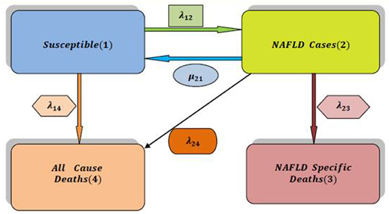
Figure 1. The simplest multistate model for analysis of NAFLD (health-illness-death process) [2].

A MATLAB code illustrating all the calculations is published in the code Ocean site at the URL: https://codeocean.com/capsule/8641183/tree/v2 with doi: 10.24433/CO.6022979.v2.

A full detailed description of a simple form of the model to enhance understanding of the difference between the two forms of the model is illustrated in a thorough explanation in the Supplementary Materials for the simple model (refer to Supplementary Material).

In this article, NAFLD is modeled as a multistage disease process consisting of nine stages, as depicted in Figure 2 [2]. As shown in Figure 2, the patient can move across the stages of the disease process. Whereas, remission rates are allowed from stage 4 (compensated liver cirrhosis) to earlier stages, the patient progresses to HCC and liver transplantation once he arrives at stage 5 (decompensated liver cirrhosis), and remission rates are not allowed. Death state can be reached from any state. The patient can move from the first 5 stages to stage 8 (HCC) with a higher rate of progression from stage 4 (CC) or stage 5 (DCC) to stage 8 (HCC) compared to the first 3 stages. A brief definition of each stage is illustrated below the figure.

FIGURE 2

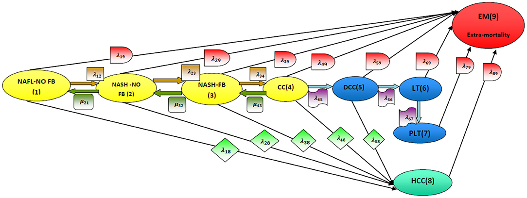
Figure 2. Disease model structure. NAFL-NO FB, non-alcoholic fatty liver with no fibrosis (stage 1); NASH-NO FB, non-alcoholic steatohepatitis with no fibrosis (stage 2); NASH-FB, non-alcoholic steatohepatitis with fibrosis (stage 3); CC, compensated cirrhosis (stage 4); DCC, decompensated cirrhosis (stage 5); LT, liver transplant (stage 6); PLT, post liver transplant (stage 7); HCC, hepatocellular carcinoma (stage 8); EM, extramortality (stage 9). [2].

NAFLD stages are modeled as time-homogenous CTMCs, that is, P_ij(Δt) depends on Δt and not on t, with constant transition intensities λ_ij over time, exponentially distributed time spent within each state and patient events following a Poisson distribution. The states are finite and can be defined or identified based on various aspects, such as clinical symptoms and invasive or non-invasive investigations. The gold-standard method for the classification of histopathological changes in the liver is invasive liver biopsy. It is presently the most trustworthy procedure for diagnosing the presence of steatohepatitis and fibrosis in patients with NAFLD [6]. The limitations of this procedure are cost, sampling error, and procedure-related morbidity and mortality. MR imaging, by spectroscopy [7] or by proton density fat fraction [8], is an excellent non-invasive technique for quantifying HS and is being widely used in NAFLD clinical trials [9]. The use of transient elastography (TE) to obtain continuous attenuation parameters is a promising tool for quantifying hepatic fat in an ambulatory setting [10]. However, non-invasive quantification of HS in patients with NAFLD is limited in routine clinical care. Additionally, one of the most recent biological markers is the keratin (K18) and its caspase-cleaved fragments (cK18). There are many scoring systems that can identify the stages of the disease process [11]. NAFLD has a higher prevalence rate in individuals with risk factors such as visceral obesity, type 2 diabetes mellitus (T2DM), dyslipidemia, hypertension, older age, male sex, and Hispanic ethnicity [12].

For simplicity, all individuals are assumed to enter the disease process at stage one, and they are all followed up with the same length of the time interval between measurements.

The article is divided into eight sections. In Section 1, the transition probabilities are thoroughly discussed. In Section 2, transition rates are clarified. In Section 3, the mean sojourn time and its variance are reviewed. In Section 4, the state probability distribution and its covariance matrix are discussed. In Section 5, the life expectancy of the patients is considered. In Section 6, the expected numbers of patients in each state are obtained. A hypothetical numerical example is used in Section 7 to illustrate the above concepts. Finally, a brief summary is comprehended in Section 8. A link to the MATLAB code is provided at the end of the article (refer to Supplementary Material, Appendix A & B).

1. Transition Probabilities

NAFLD is modeled by multistate Markov chains that define a stochastic process:

$\begin{array}{l}\left[(\text{X}(\text{t}),\text{ t}\in \text{ T})\right]\text{ over a finite state space S}=\left\{1,2,\dots ,9\right\}\\ \hfill \text{and T}=\left[0,\text{t }\right]\text{ and t }<\text{∞}.\end{array}$

The transitions can occur at any point in time and, hence, are called continuous time Markov chains, in contrast to the discrete time Markov chains in which transitions occur at fixed points in time. The rates at which these transitions occur are constant over time and, thus, are independent of t; that is, the transition of the patient from state i at time = t to state j at t = t +s where s = Δt depends on the difference between two consecutive time points. In addition, it is defined as ${\theta }_{ij}(t)=\underset{\Delta t\to 0}{lim}\frac{P_{ij}(\Delta t)-I}{\Delta t}$ or the Q matrix; while, the I matrix is the identity matrix, the thetas are the transition rates among states (in this model, they are 22 rates).

For the above multistate Markov model demonstrating the NAFLD process, the forward Kolmogorov differential Equations (1) are as follows:

$\begin{array}{l}\frac{d}{dt}P(t)=PQ=\\ \left[\begin{array}{ccccccccc}{P}_{11}& P_{12}& P_{13}& P_{14}& P_{15}& P_{16}& P_{17}& P_{18}& P_{19}\\ P_{21}& P_{22}& P_{23}& P_{24}& P_{25}& P_{26}& P_{27}& P_{28}& P_{29}\\ P_{31}& P_{32}& P_{33}& P_{34}& P_{35}& P_{36}& P_{37}& P_{38}& P_{39}\\ P_{41}& P_{42}& P_{43}& P_{44}& P_{45}& P_{46}& P_{47}& P_{48}& P_{49}\\ 0& 0& 0& 0& P_{55}& P_{56}& P_{57}& P_{58}& P_{59}\\ 0& 0& 0& 0& 0& P_{66}& P_{67}& 0& P_{69}\\ 0& 0& 0& 0& 0& 0& P_{77}& 0& P_{79}\\ 0& 0& 0& 0& 0& 0& 0& P_{88}& P_{89}\\ 0& 0& 0& 0& 0& 0& 0& 0& P_{99}\end{array}\right]\\ \left[\begin{array}{ccccccccc}-{\gamma }_1& {\lambda }_{12}& 0& 0& 0& 0& 0& {\lambda }_{18}& {\lambda }_{19}\\ {\mu }_{21}& -{\gamma }_2& {\lambda }_{23}& 0& 0& 0& 0& {\lambda }_{28}& {\lambda }_{29}\\ 0& {\mu }_{32}& -{\gamma }_3& {\lambda }_{34}& 0& 0& 0& {\lambda }_{38}& {\lambda }_{39}\\ 0& 0& {\mu }_{43}& -{\gamma }_4& {\lambda }_{45}& 0& 0& {\lambda }_{48}& {\lambda }_{49}\\ 0& 0& 0& 0& -{\gamma }_5& {\lambda }_{56}& 0& {\lambda }_{58}& {\lambda }_{59}\\ 0& 0& 0& 0& 0& -{\gamma }_6& {\lambda }_{67}& 0& {\lambda }_{69}\\ 0& 0& 0& 0& 0& 0& -{\lambda }_{79}& 0& {\lambda }_{79}\\ 0& 0& 0& 0& 0& 0& 0& -{\lambda }_{89}& {\lambda }_{89}\\ 0& 0& 0& 0& 0& 0& 0& 0& 0\end{array}\right]& (1)\end{array}$

Solving the Kolmogorov differential equations will give the transition probability matrix P_ij(t) (refer to Supplementary Material Section 1).

P_ij(t) satisfies the following properties:

1. $P_{ij}(t+s)=\sum _{i.j.l\in S}{P}_{il}(t)P_{lj}(s),\forall t\ge 0,s\ge 0,i,j,l\in S;\text{ obeying kolmogrov equations}.$

2. ${\sum }_S{P}_{ij}(t)=1.$

3. P_ij(t) ≥ 0, ∀ t ≥ 0 and i, j ∈ S.

The Q matrix satisfies the following conditions:

1. ${\sum }_S{q}_{ij}(t)=0.$

2. q_ij(t) ≥ 0 i ≠ j.

3. $-{\sum }_S{q}_{ij}(t)=q_{ii}i=j.$

where q_ij is the ( i, j) th entry in the Q matrix emphasizing that P_ij depends only on the interval between t₁ and t₂ and not on t₁.

2. Maximum Likelihood Estimation of the Q Transition Rate Matrix

Let n_ijr be the number of individuals in state i at t_r−1 and in state j at time t_r. Conditioning on the distribution of individuals among states at t₀, the likelihood function for θ is (2):

$\begin{array}{ll}L(\theta )={\displaystyle \prod _{r=1}^{\tau }}\left\{{\displaystyle \prod _{i,j=1}^{k=9}}{\left[P_{ij}(t_{r-1},t_r)\right]}^{n_{ijr}}\right\}& (2)\end{array}$

where k is the index of the number of states

$\begin{array}{l}logL(\theta )={\displaystyle \sum _{r=1}^{\tau }}{\displaystyle \sum _{i.j=1}^{k=9}}{n_{ijr}logP}_{ij}(t_{r-1},t_r)where\tau =(t_r{-t}_{r-1}).\end{array}$

According to Kalbfleisch and Lawless [13], applying the quasi-Newton method to estimate the rates mandates calculating the score function S(θ) (3), which is a vector–valued function for the required rates and is the first derivative of the log likelihood function. The second derivative of the probability transition function with respect to theta is assumed to be zero.

$\begin{array}{l}\hfill S(\theta )=\frac{\partial }{\partial {\theta }_h}logL(\theta )={\displaystyle \sum _{r=1}^{\tau }}{\displaystyle \sum _{i,j=1}^k}{n}_{ijr}\frac{\partial P_{ij}(\tau )/\partial {\theta }_h}{P_{ij}(\tau )},\\ \hfill h=1,\dots ,22while{P}_{ij}(\tau )=\frac{n_{ijr}}{n_{i+}},suchthat{n}_{i+}={\displaystyle \sum _{j=1}^k}{n}_{ijr}.\\ \hfill S(\theta )=\tau e^{\Lambda \tau }d\Lambda & (3)\end{array}$

where S(θ) is the score function.

Λ is the eigenvalue for each Q matrix in each τ (refer to Supplementary Material Section 2). Taking the second derivative of logL (θ) (4):

$\begin{array}{l}\hfill \frac{{\partial }^2}{\partial {\theta }_g\partial {\theta }_h}logL(\theta )\\ ={\displaystyle \sum _{r=1}^{\tau }}{\displaystyle \sum _{i,j=1}^k}{n}_{ijr}\left\{\frac{{\partial }^2{P}_{ij}(\tau )/\partial {\theta }_g\partial {\theta }_h}{P_{ij}(\tau )}-\frac{\partial P_{ij}(\tau )/\partial {\theta }_g\partial P_{ij}(\tau )/\partial {\theta }_h}{P_{ij}^2(\tau )}\right\}& (4)\end{array}$

Assuming the second derivative is zero and $\frac{n_{ijr}}{P_{ij}(\tau )}=n_{i+}$ where $n_{i+}=\sum _{j=1}^9{n}_{ij}$ then:

$\begin{array}{l}{M}_{ij}(\theta )=\frac{{\partial }^2}{\partial {\theta }_g\partial {\theta }_h}logL(\theta )=\\ -{\displaystyle \sum _{r=1}^{\tau }}{\displaystyle \sum _{i,j=1}^k}{n}_{i+}\frac{\partial P_{ij}(\tau )/\partial {\theta }_g\partial P_{ij}(\tau )/\partial {\theta }_h}{P_{ij}(\tau )}.\end{array}$

The quasi-Newton formula is (5).

$\begin{array}{ll}{\theta }_1={\theta }_0+{\left[M({\theta }_0)\right]}^{-1}S({\theta }_0)& (5)\end{array}$

According to Klotz and Sharples [14], the initial ${\theta }_0=\frac{n_{ijr}}{n_{i+}}for\Delta t=1.$

For this NAFLD process (refer to Supplementary Material Section 2).

3. Mean Sojourn Time

It is the mean time spent by a patient in a given state i of the process. It is calculated in relation to transition rates $\widehat{\theta }$. These times are independent and exponentially distributed random variables with mean $\frac{1}{{\lambda }_i}$ where λ_i = −λ_ii; i = 1, …, 8.

According to Kalbfleisch and Lawless [13], the asymptotic variance of this time is calculated by applying the multivariate delta method (6):

$\begin{array}{ll}var(s_i)={\left[{\left(q_{ii}\left(\widehat{\theta }\right)\right)}^{-2}\right]}^2{\displaystyle {\sum }_{h=1}^{22}{\sum }_{g=1}^{22}}\frac{\partial q_{ii}}{\partial {\theta }_g}\frac{\partial q_{ii}}{\partial {\theta }_h}{\left[M(\theta )\right]}^{-1}{|}_{\theta =\widehat{\theta }}& (6)\end{array}$

where s_i is the mean sojourn time.

For this NAFLD process (refer to Supplementary Material Section 3).

4. State Probability Distribution

According to Cassandras and Lafortune [15], it is the probability distribution for each state at a specific time point given the initial probability distribution. Thus, using the rule of total probability, a solution describing the transient behavior of a chain characterized by Q and an initial condition π(0) is obtained by direct substitution to solve (7):

$\begin{array}{ll}\pi (t)=\pi (0)P(t).& (7)\end{array}$

The stationary probability distribution when t goes to infinity or, in other words, when the process does not depend on time is obtained by differentiating both sides of the following Equation (8):

$\begin{array}{ll}\pi (t)=\pi (0)P(t)=\pi (0)e^{Qt}& (8)\end{array}$

$\text{differentiate both sides to obtain }\frac{d}{dt}\pi (t){|}_{t=0}=\pi (0)Q.$

$\begin{array}{l}\frac{d}{dt}{\pi }_i(t){|}_{t=0}\\ =\left[\begin{array}{ccccccccc}{\pi }_{0(1)}& {\pi }_{0(2)}& {\pi }_{0(3)}& {\pi }_{0(4)}& {\pi }_{0(5)}& {\pi }_{0(6)}& {\pi }_{0(7)}& {\pi }_{0(8)}& {\pi }_{0(9)}\end{array}\right]\times \\ \left[\begin{array}{ccccccccc}-{\gamma }_1& {\lambda }_{12}& 0& 0& 0& 0& 0& {\lambda }_{18}& {\lambda }_{19}\\ {\mu }_{21}& -{\gamma }_2& {\lambda }_{23}& 0& 0& 0& 0& {\lambda }_{28}& {\lambda }_{29}\\ 0& {\mu }_{32}& -{\gamma }_3& {\lambda }_{34}& 0& 0& 0& {\lambda }_{38}& {\lambda }_{39}\\ 0& 0& {\mu }_{43}& -{\gamma }_4& {\lambda }_{45}& 0& 0& {\lambda }_{48}& {\lambda }_{49}\\ 0& 0& 0& 0& -{\gamma }_5& {\lambda }_{56}& 0& {\lambda }_{58}& {\lambda }_{59}\\ 0& 0& 0& 0& 0& -{\gamma }_6& {\lambda }_{67}& 0& {\lambda }_{69}\\ 0& 0& 0& 0& 0& 0& -{\lambda }_{79}& 0& {\lambda }_{79}\\ 0& 0& 0& 0& 0& 0& 0& -{\lambda }_{89}& {\lambda }_{89}\\ 0& 0& 0& 0& 0& 0& 0& 0& 0\end{array}\right]\end{array}$

$\left[\begin{array}{ccccccccc}{\pi }_1& {\pi }_2& {\pi }_3& {\pi }_4& {\pi }_5& {\pi }_6& {\pi }_7& {\pi }_8& {\pi }_9\end{array}\right]$at a specific time point is obtained by solving this system of differential equations. Solving these differential equations for this complex chain is cumbersome.

If the limit of ${\pi }_z=\underset{t\to \infty }{lim}{\pi }_z(t)$exists, then there is a stationary or steady state distribution, and as $t\to \infty ,\frac{d}{dt}{\pi }_j(t)=0$, since π_z(t) does not depend on time. Therefore, $\frac{d}{dt}\pi (t)=\pi (t)Q$ will reduce to π(t)Q = 0. The stationary state probability distribution is obtained by solving π(t)Q = 0 subject to $\sum _{allz}{\pi }_z=1$.

For this NAFLD process (refer to Supplementary Material Section 4).

4.1. Asymptotic Covariance of the State Probability Distribution

The multivariate delta method is applied to the following function $Q^{\prime }\pi =F({\theta }_h,{\pi }_i)=0$ to obtain the asymptotic covariance matrix of the state probability distribution, as π is not a simple function of theta.

Differentiating F(θ_h, π_i) implicitly with respect to θ_h is used in the following manner (9):

$\begin{array}{ll}\frac{\partial }{\partial {\theta }_h}F({\theta }_h,{\pi }_i)=\frac{\partial }{\partial {\theta }_h}{Q}^{\prime }{\pi }_i=0.& (9)\end{array}$

$\begin{array}{l}\frac{\partial }{\partial {\theta }_h}{Q}^{\prime }{\pi }_i=[Q^{\prime }]\left[\frac{\partial }{\partial {\theta }_h}{\pi }_i\right]+{\pi }_i{\left[\frac{\partial }{\partial {\theta }_h}{Q}^{\prime }\right]}^T=0\\ \hfill let\text{'}scall{\pi }_i{\left[\frac{\partial }{\partial {\theta }_h}{Q}^{\prime }\right]}^T=C\left(\theta \right).\\ \hfill [Q^{\prime }]\left[\frac{\partial }{\partial {\theta }_h}{\pi }_i\right]+C\left(\theta \right)=0.\\ \hfill solvingfor\left[\frac{\partial }{\partial {\theta }_h}{\pi }_i\right],\\ \hfill \left[\frac{\partial }{\partial {\theta }_h}{\pi }_i\right]=-{\left[Q^{\prime }\right]}^{-1}C\left(\theta \right).\\ \hfill Let\left[\frac{\partial }{\partial {\theta }_h}{\pi }_i\right]=A\left(\theta \right).\end{array}$

By multivariate delta method

$\begin{array}{l}var(\pi )=A(\theta )var(\theta ){A(\theta )}^{\prime },wherevar(\theta )={\left[M(\theta )\right]}^{-1}.\end{array}$

For this NAFLD process: (refer to Supplementary Material Section 4.1).

5. Life Expectancy of the Patient in the NAFLD Process

The disease process is composed of eight transient states and one absorbing state (death state). So, the Q matrix is partitioned into four sets:

$\begin{array}{l}\hfill Q=\left[\begin{array}{cc}B& A\\ 0& 0\end{array}\right],\\ \hfill where\\ B=\left[\begin{array}{cccccccc}-{\gamma }_1& {\lambda }_{12}& 0& 0& 0& 0& 0& {\lambda }_{18}\\ {\mu }_{21}& -{\gamma }_2& {\lambda }_{23}& 0& 0& 0& 0& {\lambda }_{28}\\ 0& {\mu }_{32}& -{\gamma }_3& {\lambda }_{34}& 0& 0& 0& {\lambda }_{38}\\ 0& 0& {\mu }_{43}& -{\gamma }_4& {\lambda }_{45}& 0& 0& {\lambda }_{48}\\ 0& 0& 0& 0& -{\gamma }_5& {\lambda }_{56}& 0& {\lambda }_{58}\\ 0& 0& 0& 0& 0& -{\gamma }_6& {\lambda }_{67}& 0\\ 0& 0& 0& 0& 0& 0& -{\lambda }_{79}& 0\\ 0& 0& 0& 0& 0& 0& 0& -{\lambda }_{89}\end{array}\right].\end{array}$

Additionally, the differential equations can be partitioned into the following (10):

$\begin{array}{ll}\left[\acute{P}\begin{array}{cc}(t)& {\acute{P}}_k(t)\end{array}\right]=\left[\begin{array}{cc}P(t)& P_k(t)\end{array}\right]\left[\begin{array}{cc}B& A\\ 0& 0\end{array}\right]& (10)\end{array}$

B is the transition rate matrix among the transient states and column vector A is the transition rate from each transient state to the absorbing (death) state.

$\begin{array}{l}\hfill A=-B{1}^T\text{ such that }{1}^T\text{is a column vector of}(k-1)\times 1\\ \hfill \text{with all its elements equal to one}\\ \hfill \left[\acute{P}\begin{array}{cc}(t)& {\acute{P}}_k(t)\end{array}\right]=\left[\begin{array}{cc}P(t)& P_k(t)\end{array}\right]\left[\begin{array}{cc}B& A\\ 0& 0\end{array}\right]\text{can be written as}:\\ \hfill P^{\prime }(t)=P(t)Band{\acute{P}}_k(t)=P(t)A.\\ \hfill \text{The solution to }\acute{P}(t)=P(t)BisP(t)=P(0)e^{Bt}\\ \hfill then{\acute{P}}_k(t)=P(0)e^{Bt}A.\\ \hfill and{e}^{Bt}=1+Bt+\frac{{(Bt)}^2}{2!}+\frac{{(Bt)}^3}{3!}+\frac{{(Bt)}^4}{4!}+\cdots ={\displaystyle \sum _{j=0}^{\infty }}\frac{{(Bt)}^j}{j!}.\end{array}$

If τ_k is the time taken from state i to reach the absorbing death state from the initil time

$\begin{array}{l}{F}_k(t)=pr\left[{\tau }_k\le t\right]=pr\left[X(t)=k\right]=P_k(t)=1^T-P(t)1^T\\ \hfill =1^t-P(0)e^{Bt}{1}^T.\end{array}$

The moment theory for the Laplace transform can be used to obtain the mean of the time that has the above cumulative distribution function. CTMC can be written in a Laplace transform (11) such that:

$\begin{array}{l}\left[s{P}^{*}\begin{array}{cc}(s)-P(0)& s{P^{*}}_k(s)\end{array}\right]=\left[\begin{array}{cc}{P}^{*}(s)& {P^{*}}_k(s)\end{array}\right]\left[\begin{array}{cc}B& A\\ 0& 0\end{array}\right]\\ \therefore s{P}^{*}(s)-P(0)=P^{*}(s)Bands{P^{*}}_k(s)=P^{*}(s)A.& (11)\end{array}$

Rearrange:

$\begin{array}{l}\hfill \therefore s{P}^{*}(s)-P^{*}(s)B=P(0).\hfill \\ \hfill P^{*}(s)\left[sI-B\right]=P(0)\to P^{*}(s)=P(0){\left[sI-B\right]}^{-1}.\hfill \\ \hfill \therefore s{P^{*}}_k(s)=P^{*}(s)A\to {P^{*}}_k(s)\hfill \\ \hfill =\frac{1}{s}{P}^{*}(s)A=\frac{1}{s}P(0){\left[sI-B\right]}^{-1}A.\hfill \\ \hfill {F^{*}}_k(s)=\frac{1}{s}P(0){\left[sI-B\right]}^{-1}A.\hfill \\ \hfill {f^{*}}_k(s)=s{F^{*}}_k(s)=P(0){\left[sI-B\right]}^{-1}A;\hfill \\ \hfill whereA=-B{1}^T.\hfill \end{array}$

Mean time to absorption:

$\begin{array}{l}\hfill E({\tau }_k)=(-1){\frac{d{f^{*}}_k(s)}{ds}|}_{s=0}=(-1){P(0){\left[sI-B\right]}^{-2}A|}_{s=0}\\ \hfill =P(0){\left[-B\right]}^{-1}{1}^T.\end{array}$

For this NAFLD process: (refer to Supplementary Material Section 5).

6. Expected Number of Patients in Each State

Let u(0) be the size of patients in a specific state at a specific time t = 0. The initial size of patients U(0) = u_j(0), as there are eight transient states and one absorbing state, where u_j(0) is the initial size or number of patients in state j at time t = 0 given that u₉(0) = 0, i.e., the initial size of patients in state 9 (absorbing death state) is zero at initial time point t = 0. As the transition or the movement of the patients among states is independent, at the end of the whole time interval (0, t) and according to Chiang [16], there will be u_j(t) patients in the transient states at time t, and there will also be u₉(t)patients in state 9 (death state) at time t.

$\begin{array}{l}E\left[u_j(t)|u_j(0)\right]={\displaystyle \sum _{j=1,i=1}^9}{u}_j(0)P_{ij}(t),\\ \hfill i\&j=1,\dots ,9\end{array}$

For this NAFLD process: (refer to Supplementary Material Section 6).

7. Hypothetical Numerical Example

To illustrate the above concepts and discussion, a hypothetical numerical example is introduced. It does not represent real data but it is for demonstrative purposes (refer to Supplementary Material Section 7).

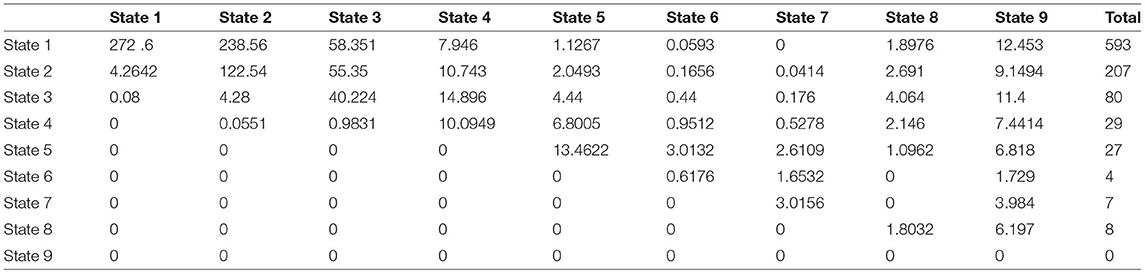
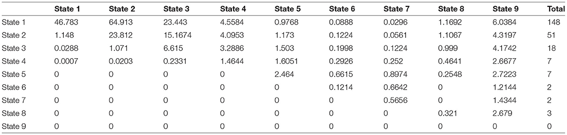
A study was conducted over 15 years on 1,050 patients with risk factors for developing NAFLD such as type 2 diabetes mellitus, obesity, and hypertension acting alone or together as a metabolic syndrome. The patients were scheduled to be followed up every year by a liver biopsy to identify the NAFLD cases, but the actual observations were recorded as shown in the (Supplementary Material). Table 1 shows the observed transition counts.

TABLE 1

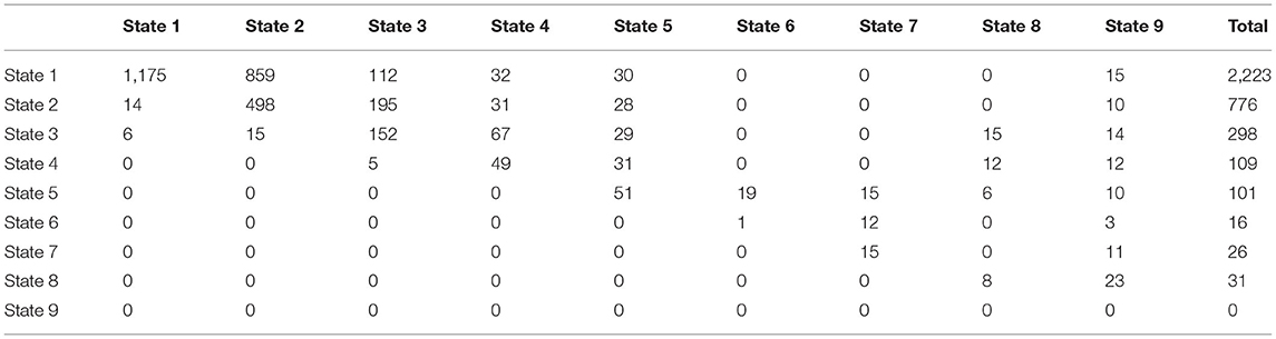
Table 1. The observed transition counts in the whole period of the study (15 years) regardless of the time interval between observations.

The observed transition rate matrix Q over the whole period of the study (15 years) is:

$\begin{array}{l}Q=\left[\begin{array}{ccccccccc}-0.3931& 0.3864& 0& 0& 0& 0& 0& 0& 0.0067\\ 0.018& -0.2808& 0.25& 0& 0& 0& 0& 0& 0.0128\\ 0& 0.05& -0.3717& 0.2248& 0& 0& 0& 0.05& 0.0469\\ 0& 0& 0.0458& -0.5502& 0.2844& 0& 0& 0.11& 0.11\\ 0& 0& 0& 0& -0.346& 0.188& 0& 0.059& 00.099\\ 0& 0& 0& 0& 0& -0.9375& 0.75& 0& 0.1875\\ 0& 0& 0& 0& 0& 0& -0.423& 0& 0.423\\ 0& 0& 0& 0& 0& 0& 0& -0.7419& 0.7419\\ 0& 0& 0& 0& 0& 0& 0& 0& 0\end{array}\right]\end{array}$

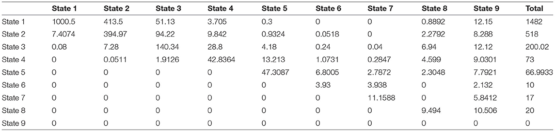
The estimated transition rate matrix $\widehat{Q}$ is:

$\begin{array}{l}\widehat{Q}=\left[\begin{array}{ccccccccc}-0.397& 0.39& 0& 0& 0& 0& 0& 0& 0.0007\\ 0.02& -0.281& 0.25& 0& 0& 0& 0& 0& 0.0011\\ 0& 0.05& -0.365& 0.225& 0& 0& 0& 0.047& 0.043\\ 0& 0& 0.041& -0.538& 0.281& 0& 0& 0.109& 0.107\\ 0& 0& 0& 0& -0.348& 0.19& 0& 0.059& 0.099\\ 0& 0& 0& 0& 0& -0.934& 0.767& 0& 0.167\\ 0& 0& 0& 0& 0& 0& -0.421& 0& 0.421\\ 0& 0& 0& 0& 0& 0& 0& -0.745& 0.745\\ 0& 0& 0& 0& 0& 0& 0& 0& 0\end{array}\right].\end{array}$

Using the above approach as illustrated in the main text and Supplementary Materials, the estimated $\widehat{Q}$ transition rate matrix is nearly approaching equality to the observed transition rate matrix.

$\begin{array}{l}var(\widehat{\theta })=1\times {10}^{-13}\left[\begin{array}{cc}{v}_1& v_2\\ v_3& v_4\end{array}\right]\end{array}$

where

$\begin{array}{l}{v}_1=\left[\begin{array}{cccccccc}0.3292& 0.0327& 0.4414& 0.0827& 0.4004& 0.0268& 0.2540& 0.1517\\ 0.0327& 0.0064& 0.0428& 0.0108& 0.0385& 0.0053& 0.0268& 0.0159\\ 0.4414& 0.0428& 0.5922& 0.1100& 0.5373& 0.0350& 0.3400& 0.2032\\ 0.0827& 0.0108& 0.1100& 0.0228& 0.0995& 0.0088& 0.0650& 0.0387\\ 0.4004& 0.0385& 0.5373& 0.0995& 0.4876& 0.0315& 0.3082& 0.1843\\ 0.0268& 0.0053& 0.0350& 0.0088& 0.0315& 0.0044& 0.0219& 0.0130\\ 0.2540& 0.0268& 0.3400& 0.0650& 0.3082& 0.0219& 0.1967& 0.1174\\ 0.1517& 0.0159& 0.2032& 0.0387& 0.1843& 0.0130& 0.1174& 0.0702\end{array}\right].\end{array}$

v₂, v₃, and v₄ are all zero matrices of size (8 by 14), (14 by 8), and (14 by 14), respectively.

Transition probability matrix at 1 year:

$\begin{array}{l}P(1)=\left[\begin{array}{ccccccccc}0.6751& 0.279& 0.0345& 0.0025& 0.0002& 0& 0& 0.0006& 0.0082\\ 0.0143& 0.7625& 0.1819& 0.0190& 0.0018& 0.0001& 0& 0.0044& 0.016\\ 0.0004& 0.0364& 0.7017& 0.144& 0.0209& 0.0012& 0.0002& 0.0347& 0.0606\\ 0& 0.0007& 0.0262& 0.5868& 0.1810& 0.0147& 0.0039& 0.0630& 0.1237\\ 0& 0& 0& 0& 0.7061& 0.1015& 0.0416& 0.0344& 0.1163\\ 0& 0& 0& 0& 0& 0.3930& 0.3938& 0& 0.2132\\ 0& 0& 0& 0& 0& 0& 0.6564& 0& 0.3436\\ 0& 0& 0& 0& 0& 0& 0& 0.4747& 0.5253\\ 0& 0& 0& 0& 0& 0& 0& 0& 1\end{array}\right].\end{array}$

Mean time spent by the patient in state 1 is ~2 years and 6 months; in state 2, the mean sojourn time is ~3 years and 6 months; in state 3, it is ~2 years and 9 months; in state 4, it is ~1 year and 10 months; in state 5, it is ~2 years and 10 months; in state 6, it is ~1 year and 1 month; in state 7, it is ~2 years and 5 months and last; in state 8, the mean sojourn time is ~1 year and 4 months.

If a cohort of 5,000 patients with NAFLD has an initial distribution of $\left[\begin{array}{ccccccccc}0.62& 0.22& 0.081& 00.03& 0.028& 0.005& 00.007& 0.009& 0\end{array}\right]$and the initial counts of patients in each state are $\left[\begin{array}{ccccccccc}3100& 1100& 405& 150& 140& 25& 35& 45& 0\end{array}\right],$ then at 1 year, the state probability distribution is $\left[\begin{array}{ccccccccc}00.4217& 0.3437& 0.1191& 00.035& 0.0274& 0.0054& 00.0079& 0.0112& 0.0287\end{array}\right]$and the expected counts of patients are $\left[\begin{array}{ccccccccc}2109& 1718& 595& 175& 137& 27& 39& 56& 144\end{array}\right]$.

To calculate the goodness of fit for the multistate model used in this example, it is similar to the procedure used in the contingency table, and it is calculated in each interval and then summed:

Step 1: H₀ = future state does not depend on the current state.       H₁ = future state depends on the current state.

Step 2: Calculate the P_ij(Δt = 1)

$\begin{array}{l}{P}_{ij}(\Delta t=1)=\left[\begin{array}{ccccccccc}0.6751& 0.279& 0.0345& 0.0025& 0.0002& 0& 0& 0.0006& 0.0082\\ 0.0143& 0.7625& 0.1819& 0.0190& 0.0018& 0.0001& 0& 0.0044& 0.016\\ 0.0004& 0.0364& 0.7017& 0.144& 0.0209& 0.0012& 0.0002& 0.0347& 0.0606\\ 0& 0.0007& 0.0262& 0.5868& 0.1810& 0.0147& 0.0039& 0.0630& 0.1237\\ 0& 0& 0& 0& 0.7061& 0.1015& 0.0416& 0.0344& 0.1163\\ 0& 0& 0& 0& 0& 0.3930& 0.3938& 0& 0.2132\\ 0& 0& 0& 0& 0& 0& 0.6564& 0& 0.3436\\ 0& 0& 0& 0& 0& 0& 0& 0.4747& 0.5253\\ 0& 0& 0& 0& 0& 0& 0& 0& 1\end{array}\right].\end{array}$

Step 3: Calculate the expected counts in this interval by multiplying each row in the probability matrix with the corresponding total marginal counts in the observed transition counts matrix in the same interval to obtain the expected counts.

Step 4: Apply ${\displaystyle \sum _{i=1}^9\sum _{j=1}^9}\frac{{(O_{ij}-E_{ij})}^2}{E_{ij}}=2219.118~{\chi }_{(9-1)(9-1)(0.05)}^2$.

The same steps are used for the observed transition counts in Δt = 2 and Δt = 3 with the following results:

$\begin{array}{l}{P}_{ij}(\Delta t=2)=\left[\begin{array}{ccccccccc}0.4597& 0.4023& 0.0984& 0.0134& 0.0019& 0.0001& 0.0000& 0.0032& 0.0210\\ 0.0206& 0.5920& 0.2674& 0.0519& 0.0099& 0.0008& 0.0002& 0.013& 0.0442\\ 0.001& 0.0535& 0.5028& 0.1862& 0.0555& 0.0055& 0.0022& 0.0508& 0.1425\\ 0& 0.0019& 0.0339& 0.3481& 0.2345& 0.0328& 0.0182& 0.074& 0.2566\\ 0& 0& 0& 0& 0.4986& 0.1116& 0.0967& 0.0406& 0.2525\\ 0& 0& 0& 0& 0& 0.1544& 0.4133& 0& 0.4323\\ 0& 0& 0& 0& 0& 0& 0.4308& 0& 0.5692\\ 0& 0& 0& 0& 0& 0& 0& 0.2254& 0.7746\\ 0& 0& 0& 0& 0& 0& 0& 0& 1\end{array}\right].\end{array}$

The expected counts are:

$applying:{\displaystyle \sum _{i=1}^9\sum _{j=1}^9}\frac{{(O_{ij}-E_{ij})}^2}{E_{ij}}=158.571~{\chi }_{(9-1)(9-1)(0.05)}^2$.

The same steps are used for the observed transition counts Δt = 3 in with the following results:

$\begin{array}{l}{P}_{ij}(\Delta t=3)=\left[\begin{array}{ccccccccc}0.3161& 0.4386& 0.1584& 0.0308& 0.0066& 0.0006& 0.0002& 0.0079& 0.0408\\ 0.0225& 0.4669& 0.2974& 0.0803& 0.0803& 0.0024& 0.0011& 0.0217& 0.0847\\ 0.0016& 0.0595& 0.3675& 0.1827& 0.0835& 0.0111& 0.0068& 0.0555& 0.2319\\ 0.0001& 0.0029& 0.0333& 0.2092& 0.2293& 0.0418& 0.036& 0.0663& 0.3811\\ 0& 0& 0& 0& 0.352& 0.0945& 0.1282& 0.0364& 0.3889\\ 0& 0& 0& 0& 0& 0.0607& 0.3321& 0& 0.6072\\ 0& 0& 0& 0& 0& 0& 0.2828& 0& 0.7172\\ 0& 0& 0& 0& 0& 0& 0& 0.107& 0.893\\ 0& 0& 0& 0& 0& 0& 0& 0& 1\end{array}\right].\end{array}$

The expected counts are:

$applying:{\displaystyle \sum _{i=1}^9\sum _{j=1}^9}\frac{{(O_{ij}-E_{ij})}^2}{E_{ij}}=65.37~{\chi }_{(9-1)(9-1)(0.05)}^2$.

Step 5: Sum up the above results to get:

$\begin{array}{l}{\displaystyle \sum _{i=1}^9}{\displaystyle \sum _{j=1}^9}{\displaystyle \sum _{l=1}^{t=3}}\frac{{(O_{ijl}-E_{ijl})}^2}{E_{ijl}}=2443.06~{\chi }_{(df=192)(0.05)}^2.\end{array}$

Therefore, from the above results, the null hypothesis is rejected, whereas the alternative hypothesis is accepted, and the model fits the data to mean that the future state depends on the current state with the estimated transition rate and probability matrices as obtained.

8. Conclusion and Summary

Continuous time Markov chains are suitable mathematical and statistical tools to be used for the analysis of disease evolution over time. CTMCs are the type of multistate model utilized to study this evolution in patients with NAFLD, with the main phenotypes being NAFL and NASH, as well as to study the associated presence of fibrosis and its stages. The prevalence of NAFLD is rapidly increasing worldwide and parallels the epidemics of obesity and type 2 diabetes. Metabolic syndrome is a well-known risk factor.

In this study, NAFLD is modeled in a more elaborative expanded form, which includes nine states: the first eight states are the states of disease progression as time elapses, while the ninth state is the death state. The importance of such analysis is that health policy makers can predict the number of affected patients at each stage, the needed investigations and medications for each of them, and the costs and budgets that medical insurance should assign to this disease burden. This analysis is of great value and benefit to physicians, as they can conduct longitudinal studies to explore further investigations that better define each stage specifically and efficiently and to explore further treatment needed for each stage. An example of a non-invasive diagnostic tool is the circulating level of cytokeratin-18 fragments; although promising, it is not available in a clinical care setting, and there is no established cutoff value for identifying NASH [17]. Genetic polymorphism of patatin-like phospholipase domain-containing protein 3 gene variants (PNPLA-3) is associated with NASH and advanced fibrosis; however, testing for these variants in routine clinical care is not supported and needs further study.

A hypothetical example of factitious non-real data is used to emphasize the attributes that need to be estimated:

❖ Transition rate matrix among the various states.

❖ Transition probability matrix among states.

❖ Mean sojourn time in each state.

❖ Life expectancy in each state; in other words, mean time to absorption (death state).

❖ Expected number of patients in each state.

❖ State probability distribution at specific time points in the future.

Such analysis may give better insights to physicians, especially when new drug classes will soon be released on the market. What drug classes are to be used first? How can the disease be monitored throughout the journey of treatment? What investigations are to be used in such monitoring? How to modify the drug treatment? What is the target that needs to be achieved, and how can this target be maintained? Moreover, in the late stage of the disease, when patients suffer from decompensated liver cirrhosis, liver transplantation is the treatment of choice to such patients, which increases the economic burden of NAFLD, as was the disease course during treatment in the early stages. Additionally, a load of what are the best economic non-invasive tests to be used in primary health care units for stratification and identification of high-risk patients, whether to perform genetic tests in health insurance settings, and when to refer for liver biopsy in secondary or special clinics should be considered. All these questions can be answered from longitudinal studies conducted on susceptible individuals. Over and above, some of the recently investigated non-invasive scoring systems of fibrosis need further external validation to be generalized in ethnicities other than the one tested upon. There are some controversies regarding the cutoff points of these scoring systems among countries and ethnicities within the same country. Although liver biopsy is considered the standard method for the diagnosis of NAFLD and staging it, its limitations encourage the development of various non-invasive tests, which necessitate better correlation between the findings obtained from the biopsy and the results of these tests to minimize misclassification errors, which hamper good diagnosis and prognosis of the patient. These tests should be easy, feasible, convenient, and have a high safety profile to be used repeatedly in patients for follow-up in such longitudinal studies.

A multistate model represented by CTMC is a valuable statistical methodology for longitudinal studies in medical research to better comprehend and understand the pathophysiology or the mechanism of the NAFLD process, and the interactions between the different modifiers, either external or internal modifiers. The external modifiers reside in bad dietary habits with excessive fat and carbohydrate ingestion, and sedentary life, whereas the internal modifiers are represented in genetic factors affecting the metabolism of the food stuff (fat and carbohydrates) and other cellular functions, such as risk factors for fibrogenesis (formation of fibrous tissue); fibrosis is a detrimental predictor factor for disease progression to liver cirrhosis and its complications. The importance of such understanding has a great impact on revealing the genes that must be tested if ever needed, for whom to do such a test, and should it be in the utilities or services offered by medical insurance. Moreover, should the degradation byproducts resulting from extracellular matrix destruction be used in routine clinical practice to mirror the fibrosis stages?

In Egypt, there are scarce data or maybe no available data about the prevalence of NAFLD and its phenotypes. Guidelines for risk stratification and identification are also lacking. Thus, more longitudinal studies are needed to address these issues.

Multistate models can also be used for the analysis of competing risks of death in such patients, as the first and second most common causes of death in patients with NAFLD are cardiovascular diseases (CVDs) and kidney diseases, whereas liver-related mortality is the third most common cause of death.

Other statistical methodologies, such as semi-Markov and hidden Markov chains, can be used to model NAFLD, especially hidden Markov CTMC can be used to model misclassification errors encountered in studies analyzed by time-homogenous CTMC.

Hint: A MATLAB code is edited to calculate the statistical indices in the hypothetical example. The code can be found published in the code ocean site with the following URL: https://codeocean.com/capsule/7628018/tree/v3; doi: 10.24433/CO.7719785.v3.

Author Contributions

IA carried the conceptualization by formulating the goals, aims of the research article, formal analysis by applying the statistical, mathematical and computational techniques to synthesize and analyze the hypothetical data, carried the methodology by creating the model, software programming and implementation, supervision, writing, drafting, editing, preparation, and creation of the presenting work.

Conflict of Interest

The author declares that the research was conducted in the absence of any commercial or financial relationships that could be construed as a potential conflict of interest.

Publisher's Note

All claims expressed in this article are solely those of the authors and do not necessarily represent those of their affiliated organizations, or those of the publisher, the editors and the reviewers. Any product that may be evaluated in this article, or claim that may be made by its manufacturer, is not guaranteed or endorsed by the publisher.

Supplementary Material

The Supplementary Material for this article can be found online at: https://www.frontiersin.org/articles/10.3389/fams.2021.766085/full#supplementary-material

Supplementary Data-sheet 1. Excel sheet for the timeline of the participants.

Supplementary Data-sheet 2. Supplementary material for the simple data model.

Supplementary Data-sheet 3. Supplementary material for the expanded model.

Supplementary Data-sheet 4. MATLAB code, Appendix A (rate) and Appendix B (probability).

Abbreviations

CC, compensated cirrhosis (stage 4); CTMCs, continuous time Markov chains; CVS, cardiovascular disease; DCC, decompensated cirrhosis (stage 5); EASD, European Association for the Study of Diabetes; EASL, European Association for the Study of Liver; EASO, European Association for the Study of Obesity; EM, extramortality (stage 9); HCC, hepatocellular carcinoma (stage 8); HS, hepatic steatosis; LT, liver transplant (stage 6); NAFLD, non-alcoholic fatty liver disease; NAFL-NO FB, non-alcoholic fatty liver with no fibrosis (stage 1); NASH, non-alcoholic steatohepatitis; NASH-NO FB, non-alcoholic steatohepatitis with no fibrosis (stage 2); NASH-FB, non-alcoholic steatohepatitis with fibrosis (stage 3); PLT, postliver transplant (stage 7); PNPLA-3, patatin-like phospholipase domain containing protein 3 gene variants; TE, transient elastography; T2DM, type 2 diabetes mellitus.

References

1. Estes C, Razavi H, Loomba R, Younossi Z, Sanyal AJ. Modeling the epidemic of nonalcoholic fatty liver disease demonstrates an exponential increase in burden of disease. Hepatology. (2018) 67:123–33. doi: 10.1002/hep.29466

PubMed Abstract | CrossRef Full Text | Google Scholar

2. Younossi ZM, Blissett D, Blissett R, Henry L, Stepanova M, Younossi Y, et al. The economic and clinical burden of nonalcoholic fatty liver disease in the United States and Europe. Hepatology. (2016) 64:1577–86. doi: 10.1002/hep.28785

PubMed Abstract | CrossRef Full Text | Google Scholar

3. Chalasani N, Younossi Z, Lavine JE, Charlton M, Cusi K, Rinella M, et al. The diagnosis and management of nonalcoholic fatty liver disease: practice guidance from the American Association for the Study of Liver Diseases. Hepatology. (2018) 67:328–57. doi: 10.1002/hep.29367

PubMed Abstract | CrossRef Full Text | Google Scholar

4. Association E, Association E, Easd D, Association E, Easo O. Clinical practice guidelines EASL – EASD – EASO clinical practice guidelines for the management of non-alcoholic fatty liver disease q. J Hepatol. (2016) 64:1388–402. doi: 10.1016/j.jhep.2015.11.004

PubMed Abstract | CrossRef Full Text | Google Scholar

5. Attia IM. Continuous time markov chains for analysis of non-alcoholic fatty liver disease evolution. Int J Res Eng Sci. (2021) 9:1–23.

Google Scholar

6. Chalasani N, Wilson L, Kleiner DE, Cummings OW, Brunt EM, Ünalp A, et al. Relationship of steatosis grade and zonal location to histological features of steatohepatitis in adult patients with non-alcoholic fatty liver disease. J Hepatol. (2008) 48:829–34. doi: 10.1016/j.jhep.2008.01.016

PubMed Abstract | CrossRef Full Text | Google Scholar

7. Reeder SB, Cruite I, Hamilton G, Sirlin CB. Quantitative assessment of liver fat with magnetic resonance imaging and spectroscopy. J Magn Reson Imag. (2011) 34:729–49. doi: 10.1002/jmri.22580

PubMed Abstract | CrossRef Full Text | Google Scholar

8. Idilman IS, Keskin O, Celik A, Savas B, Halil Elhan A, Idilman R, et al. A comparison of liver fat content as determined by magnetic resonance imaging-proton density fat fraction and MRS versus liver histology in non-alcoholic fatty liver disease. Acta radiol. (2016) 57:271–8. doi: 10.1177/0284185115580488

PubMed Abstract | CrossRef Full Text | Google Scholar

9. Noureddin M, Lam J, Peterson MR, Middleton M, Hamilton G, Le T, et al. Utility of magnetic resonance imaging versus histology for quantifying changes in liver fat in nonalcoholic fatty liver disease trials. Hepatology. (2013) 58:1930–40. doi: 10.1002/hep.26455

PubMed Abstract | CrossRef Full Text | Google Scholar

10. Lédinghen Vde, Wong GL, Vergniol J, Chan HL, Hiriart J, Chan AW, et al. Controlled attenuation parameter for the diagnosis of steatosis in non-alcoholic fatty liver disease. J Gastroenterol Hepatol. (2016) 31:848–55. doi: 10.1111/jgh.13219

PubMed Abstract | CrossRef Full Text | Google Scholar

11. Paul J. Recent advances in non-invasive diagnosis and medical management of non-alcoholic fatty liver disease in adult. Egypt Liv J. (2020) 10:43. doi: 10.1186/s43066-020-00043-x

CrossRef Full Text | Google Scholar

12. Dongiovanni PM, Anstee Q, Valenti L. Genetic predisposition in NAFLD and NASH: impact on severity of liver disease and response to treatment. Curr Pharmaceut Design. (2013) 19:5219–38. doi: 10.2174/13816128113199990381

PubMed Abstract | CrossRef Full Text | Google Scholar

13. Kalbfleisch JD, Lawless JF. The analysis of panel data under a Markov assumption. J Am Stat Assoc. (1985) 80:863–71. doi: 10.1080/01621459.1985.10478195

CrossRef Full Text | Google Scholar

14. Klotz JH, Sharples LD. Estimation for a Markov heart transplant model. J Royal Statist Soc Ser D. (1994) 43:431–8. doi: 10.2307/2348579

PubMed Abstract | CrossRef Full Text | Google Scholar

15. Cassandras CG, Lafortune S. Introduction to Discrete Event Systems. Berlin: Springer Science & Business Media (2009). doi: 10.1007/978-0-387-68612-7

CrossRef Full Text | Google Scholar

16. Chiang CL. Introduction to Stochastic Processes in Biostatistics. Hoboken, NJ: Wiley, & Sons, Inc. (1968).

Google Scholar

17. Musso G, Gambino R, Cassader M, Pagano G. Meta-analysis: natural history of non-alcoholic fatty liver disease (NAFLD) and diagnostic accuracy of non-invasive tests for liver disease severity. Ann Med. (2011) 43:617–49. doi: 10.3109/07853890.2010.518623

PubMed Abstract | CrossRef Full Text | Google Scholar