1D Generalised Burgers-Huxley: Proposed Solutions Revisited and Numerical Solution Using FTCS and NSFD Methods

1. Introduction

The study of nonlinear partial differential equation continues to fascinate many researchers due to their ubiquitous application in every area of science and technology. Because of their complexity, many of these nonlinear partial differential equations do not always have explicit solutions using a known finite combination of elementary functions [1]. Some non linear partial differential equations, on the other hand, become integrable following a symbolic transformation. The analytical solution becomes available in this instance. Some analyses of most numerical and semi-analytical methods are studied using the heat equation. The linearity of this differential equation makes it a test case for many problems, it takes the form

$\begin{array}{ll}\frac{\partial u}{\partial t}=D\frac{{\partial }^{2}u}{\partial x^2},& (1)\end{array}$

where D is the diffusivity term or coefficient of diffusion. Burgers [2] while studying turbulence in flow resulted in the investigation of a non linear partial differential equation that contains an advective term in addition to the diffusion term and it may be regarded as a prototype in the theory of nonlinear diffusive waves. The equation takes the form

$\begin{array}{ll}\frac{\partial u}{\partial t}=-\alpha u\frac{\partial u}{\partial x}+D\frac{{\partial }^{2}u}{\partial x^2}.& (2)\end{array}$

Many approximate solutions have been documented for Equation (2) subject to different initial and boundary conditions, we mention the works of Abazari and Borhanifar [3] and Mukundan and Awasthi [4].

The FitzHugh-Nagumo model is a well-known reaction-diffusion system proposed by Hodgkin and Huxley [5] for the conduction of electrical impulses through a nerve fibre. A decade later, FitzHugh [6] and Nagumo et al. [7] solved the challenge by reducing the original four-variable system to a simplified model with only two variables. The differential equation is expressed as

$\begin{array}{ll}\frac{\partial u}{\partial t}=D\frac{{\partial }^{2}u}{\partial x^2}+\beta u(1-u)(u-\gamma ).& (3)\end{array}$

The Newell-Whitehead-Segel equation is applicable in nonlinear systems that describe the emergence of stripe patterns. This equation, on the other hand, is used as a mathematical model in a variety of systems, including Rayleigh-Benard convection, chemical reactions, and Faraday instability, and is given by

$\begin{array}{ll}\frac{\partial u}{\partial t}=D\frac{{\partial }^{2}u}{\partial x^2}+\beta u(1-u)(u+1).& (4)\end{array}$

The generalised Huxley equation which models the propagation of neural pulses, the motion of liquid crystal walls, and the dynamics of nerve fibres is expressed as

$\begin{array}{ll}\frac{\partial u}{\partial t}=D\frac{{\partial }^{2}u}{\partial x^2}+\beta u(1-u^{\delta })(u^{\delta }-\gamma ).& (5)\end{array}$

We note here that δ is an arbitrary constant. The nonlinear partial differential equation which generalises (Equations 1–5) and can be thought of as an archetypal equation for explaining the interplay between reaction mechanisms, convection effects, and diffusion transport is called the generalised Burgers-Huxley which takes the form

$\begin{array}{ll}\frac{\partial u}{\partial t}=D\frac{{\partial }^{2}u}{\partial x^2}-\alpha u^{\delta }\frac{\partial u}{\partial x}+\beta u(1-u^{\delta })(u^{\delta }-\gamma ).& (6)\end{array}$

Equation (6) can as well be thought of as a combination of Burger's equation with advective term and Huxley's equation with non linear reaction term with diffusion, hence the name. It is worth noting that, for δ = 1, Equation (6) yields the Burgers-Huxley equation. Wang et al. [8] obtained a closed form solution for Equation (6) and all of its variances. There have been many semi-analytical and numerical methods used in obtaining an approximate solution to the generalised Burgers-Huxley equation, many authors have compared some numerical solutions to the exact solution obtained in Wang et al. [8] and these works are [9–18], among many others. However, there is a minor discrepancy between the closed form solution obtained by Wang et al. [8] and the one obtained by Deng [19] using the first-integral approach. To the best of our knowledge, few researchers have compared their methods with the exact solution in [19], these include [20] using the modified exponential finite difference method, Ervin et al. [21], and Nourazar et al. [22] using the homotopy perturbation method.

Many drawbacks of the approximation analytical approaches include slow convergence at long propagation t, expensive computer memory usage, and difficulty in finding a closed form formula for the resulting series expression ([9, 10]). To this end, we cannot overemphasise the need for analysing the two proposed solutions from Wang et al. [8] and Deng [19]. In this study, we will obtain solution of the generalised Burgers-Huxley equation using the classical finite difference scheme (FTCS) and non-standard finite difference scheme (NSFD).

2. Organisation of the Paper

The structure of the paper is as follows. In section 3, we present the numerical experiment and describe some estimation tools. Section 4 is devoted to the analysis of the two proposed solutions. In section 5, we present the two numerical methods (FTCS and NSFD) and study some of their properties. We present the numerical results from FTCS and NSFD schemes using the reference solution of Wang et al. [8] as a benchmark in section 6 and the proposed solution of Deng [19] as a measure in section 7. Section 8 contains the dynamics of the travelling wave phenomenon of the Burgers-Huxley equation. Conclusion and final remarks of this study are given in section 9.

3. Numerical Experiment

We solve the generalised 1-D Burgers-Huxley Equation (6) which is given by

$\begin{array}{ll}\frac{\partial u}{\partial t}=D\frac{{\partial }^{2}u}{\partial x^2}-\alpha u^{\delta }\frac{\partial u}{\partial x}+\beta (1+\gamma )u^{1+\delta }-\beta \gamma u-\beta u^{2\delta +1},& (7)\end{array}$

subject to the following initial conditions

$\begin{array}{ll}u(x,0)={\displaystyle [\frac{\gamma }{2}+\frac{\gamma }{2}tanh\left\{\sigma \gamma x\right\}{]}^{\frac{1}{\delta }}},& (8)\end{array}$

where α > 0, β > 0, 0 < γ < 1, and δ > 0 is a positive constant, x ∈ [0, 1] and t ≥ 0. The boundary conditions are obtained from exact solution.

Wang et al. [8] used the non linear transformation to obtain a closed form solution for Equation (6) given as

$\begin{array}{l}{u}_1(x,t)\\ ={\displaystyle [\frac{\gamma }{2}+\frac{\gamma }{2}tanh\{\sigma \gamma (x-\{\frac{(\alpha +\rho )\gamma +(1+\delta )(\alpha -\rho )}{2(1+\delta )}\left\}t\right)\}{]}^{\frac{1}{\delta }}},& (9)\end{array}$

where $\sigma =\frac{\delta (\rho -\alpha )}{4(1+\delta )}$ and $\rho =\sqrt{{\alpha }^2+4\beta (1+\delta )}$.

Deng [19] claimed there is a minor error in the proposed solution given by Wang et al. [8] using the first-integral approach, which is based on the ring theory of commutative algebra. Deng [19] presented a new proposed solution given as

$\begin{array}{l}{u}_2(x,t)\\ ={\displaystyle [\frac{\gamma }{2}+\frac{\gamma }{2}tanh\{\sigma \gamma (x-\{\frac{(\alpha -\rho )\gamma +(1+\delta )(\alpha +\rho )}{2(1+\delta )}\left\}t\right)\}{]}^{\frac{1}{\delta }}},& (10)\end{array}$

where $\sigma =\frac{\delta (\rho -\alpha )}{4(1+\delta )}$ and $\rho =\sqrt{{\alpha }^2+4\beta (1+\delta )}$.

The closed-form expressions are given in Equations (9) and (10) both lie in the interval $(0,{\gamma }^{\frac{1}{\delta }})$, refer to the work of Ervin et al. [21]. We fix the coefficient of diffusion to be equal to one and we obtain the solution of generalised Burgers-Huxley equation in three distinct regimes using two finite difference methods. In this study, we consider three different cases as follows:

(1) α = 1.0, β = 1.0, γ = 0.01, δ = 4.0.

(2) α = 1.0, β = 5.0 (β > α), γ = 0.01, δ = 4.0.

(3) α = 5.0 (α > β), β = 1.0, γ = 0.01, δ = 4.0.

We used finite difference technique; Forward time central space (FTCS) and non-standard approaches in obtaining numerical solutions for the numerical experiment. The solution domains are discretised into cells as (x_j, t_n), where x_j = jh, ; (j = 1, 2, ..., N) and t_n = nk, ; (n = 1, 2, ...), where $h=\frac{1-0}{N-1}$ is the spatial mesh size and the values of h selected for computations are explicitly specified for each instance. The temporal step size is denoted by k. The following estimation techniques were used to assess the accuracy of the schemes as well as to check the exact solution with oversight

$\begin{array}{l}\text{Absolute Error}=|u(x,t)-U(x_j,t_n),|\end{array}$

$\begin{array}{ll}{L}_1=h{\displaystyle \sum _{j=1}^N}|u(x,t)-U(x_j,t_n)|,& (11)\end{array}$

and

$\begin{array}{l}{L}_{\infty }=max|u(x,t)-U(x_j,t_n)|.\end{array}$

where u(x, t) and U(x_j, t_n) are the exact and numerical solutions, respectively.

The rate of convergence in space and time are computed using

$\begin{array}{ll}{R}^T=\frac{ln{\displaystyle \left(\frac{E_k}{E_{\frac{k}{2}}}\right)}}{ln{\displaystyle \left(\frac{k}{0.5k}\right)}},& (12)\end{array}$

where E_k = ∥L_∞∥ stands for maximum norm errors at grid point k. All numerical simulations are done in MATLAB computing platform on an Intel Core-i5, 2.50 GHz PC with 5GB RAM. We use the two different proposed solutions from Wang et al. [8] and Deng [19] in order to test the performances of our two finite difference methods.

4. Analysis of the Proposed Solutions

Before we begin solving a differential equation, we must first answer three basic questions which are due to Hadamard [23]. However, we keep in mind that non linear partial differential equations may have multiple solutions in different space functions. For example, a problem may have multiple solutions, only one of which is bounded. We would argue the uniqueness of the solution in the space of bounded functions. This is the case of the closed form solution provided in Wang et al. [8] and Deng [19]. The question of well-posedness, existence, and uniqueness of the solution to the Burgers-Huxley Equation (7) has been recently reported by Mohan and Khan [24]. One classic test for possible closed form solution to any differential equation is the Painleve test, which informs us about the possible integrability of the differential equation.

In this section, we will subject the two proposed solutions in Equations (9) and (10) to test using the ansatz technique on the Burgers-Huxley equation. We consider the case where D = β = δ = 1 and γ = 1, we have our equation now as

$\begin{array}{ll}\frac{\partial u}{\partial t}-\frac{{\partial }^{2}u}{\partial x^2}+\alpha u\frac{\partial u}{\partial x}-2u^2+u+u^3=0.& (13)\end{array}$

Using the closed form expression of Wang et al. [8], we assume the solution of Equation (13) to be

$\begin{array}{ll}{u}_1(x,t)={\displaystyle [\frac{1}{2}+\frac{1}{2}tanh\{\sigma (x-\{\frac{3\alpha -\rho }{4}\left\}t\right)\left\}\right]},& (14)\end{array}$

where $\sigma =\frac{\rho -\alpha }{8}$ and $\rho =\sqrt{{\alpha }^2+8}$. By substituting Equation (14) into Equation (13) and using the Maple symbolic package in differentiating term by term before simplification, we obtain

$\begin{array}{l}\frac{\partial u}{\partial t}-\frac{{\partial }^{2}u}{\partial x^2}+\alpha u\frac{\partial u}{\partial x}-2u^2+u+u^3\\ =\frac{8-\rho \alpha +{\alpha }^2}{{\displaystyle 32cosh\left[\right(\frac{\rho }{8}-\frac{\alpha }{8}\left)\right(x-\frac{3\alpha t}{4}+\frac{\rho t}{4}){]}^2}}.& (15)\end{array}$

By using the closed form expression of Deng [19], we assume the solution of Equation (13) in the form

$\begin{array}{ll}{u}_2(x,t)={\displaystyle [\frac{1}{2}+\frac{1}{2}tanh\{\sigma (x-\{\frac{3\alpha +\rho )}{4}\left\}t\right)\left\}\right]},& (16)\end{array}$

we substitute the assumed solution Equation (16) into Equation (13) and using the Maple symbolic package to differentiate before simplification of terms, we obtain

$\begin{array}{ll}\frac{\partial u}{\partial t}-\frac{{\partial }^{2}u}{\partial x^2}+\alpha u\frac{\partial u}{\partial x}-2u^2+u+u^3=0.& (17)\end{array}$

REMARK 1. The supposed solution using Deng [19] closed-form expression satisfy Equation (13). However, the assumed solution utilising the closed-form expression of Wang et al. [8] does not satisfy Equation (13). We expect the remainder to be zero but obtained some terms on the right hand side of Equation (15).

Figure 1 gives the plots of the remainder from the two proposed solutions using the three test cases. We observed that remainder becomes extremely small, around (10⁻¹³) in case of Deng [19] but this is not the case for [8] proposed solution.

FIGURE 1

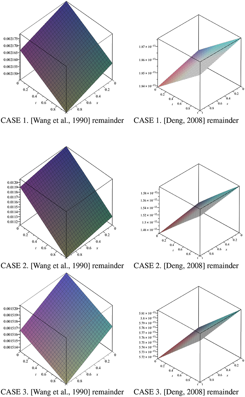
Figure 1. 3D plots of the remainder for the two proposed solutions of Wang et al. [8] and Deng [19] for the three cases using x ∈ [0, 1] and t ∈ [0, 1].

5. Numerical Methods

The study of stability, consistency, positivity, and boundedness of NSFD for the case δ = 4 was done in Appadu et al. [25], we have reproduced some of the main analyses.

5.1. FTCS Scheme

Using the FTCS scheme for Equation (7), we have

$\begin{array}{l}\frac{U_j^{n+1}-U_j^n}{k}={\displaystyle \left(\frac{U_{j+1}^n-2U_j^n+U_{j-1}^n}{h^2}\right)}-\alpha {(U_j^n)}^{\delta }\frac{U_{j+1}^n-U_{j-1}^n}{2h}\\ +\beta (1+\gamma ){(U_j^n)}^{\delta +1}-\beta \gamma U_j^n-\beta {(U_j^n)}^{2\delta +1}.& (18)\end{array}$

By making $U_j^{n+1}$ the subject, we have

$\begin{array}{l}{U}_j^{n+1}=U_j^n+\frac{k}{h^2}{\displaystyle (U_{j+1}^n-2U_j^n+U_{j-1}^n)}\\ -\frac{k\alpha }{2h}{(U_j^n)}^{\delta }{\displaystyle (U_{j+1}^n-U_{j-1}^n)}+k\beta (1+\gamma ){(U_j^n)}^{\delta +1}\\ -k\beta \gamma U_j^n-k\beta {(U_j^n)}^{2\delta +1}.& (19)\end{array}$

By using the freezing coefficient method and Von-Neumann stability analysis, we obtain the amplification factor as

$\begin{array}{l}\xi =1-I\frac{k\alpha }{h}{U}_{max}sinw+\frac{k}{h^2}(2cosw-2)\\ +k\beta {(U_{max})}^4(1+\gamma )-k\beta \gamma -k\beta {(U_{max})}^8.& (20)\end{array}$

Since $0\le U(x_j,t_n)\le {\gamma }^{1/\delta }$, it follows that $U_{max}={\gamma }^{1/4}$. On simplification, we obtain

$\begin{array}{ll}\mid \xi \mid =\sqrt{{\displaystyle (1-\frac{4k}{h^2}{sin}^2\frac{w}{2}{)}^2}+{\displaystyle (\frac{k\alpha }{h}sinw{)}^2}}.& (21)\end{array}$

Stability is guaranteed when 0 ≤ ∣ξ∣ ≤ 1 for w = [−π, π]. Region of stability is k ≤ 0.005. We next study the consistency.

We expand using Taylor's series expansion around (t_n, x_j) using Equation (19) and obtain

$\begin{array}{l}U+k{U}_t+\frac{k^2}{2}{U}_{tt}+\frac{k^3}{6}{U}_{ttt}+{O}(k^4)\\ =U+\frac{k}{h^2}{\displaystyle (h^2{U}_{xx}+\frac{h^4}{12}{U}_{xxxx}+{O}(h^6))}\\ -\frac{k\alpha }{2h}{U}^{\delta }{\displaystyle (2h{U}_x+\frac{1}{3}{h}^3{U}_{xxx}+{O}(h^5))}+k\beta (1+\gamma )U^{\delta +1}\\ -k\beta \gamma U-k\beta U^{2\delta +1}.& (22)\end{array}$

Dividing throughout by k and simplifying, we have

$\begin{array}{l}{U}_t-U_{xx}+\alpha U^{\delta }{U}_x-\beta (1+\gamma )U^{\delta +1}+\beta \gamma U+\beta U^{2\delta +1}\\ =-\frac{k}{2}{U}_{tt}-\frac{k^2}{6}{U}_{ttt}-\alpha \frac{h^2}{6}{U}^{\delta }{U}_{xxx}+\frac{h^2}{12}{U}_{xxxx}+{O}(k^3)\\ +{O}(h^4),& (23)\end{array}$

and as k, h → 0, we recover the generalised Burgers-Huxley equation. We note that the FTCS scheme is first-order accurate in time and second-order accurate in space.

REMARK 2. The generalisation of Equation (18) to a higher dimension is quite straight-forward. In ℝ^m, the approximate solution in the reaction term becomes $U_{\left\{j_1,j_2,\cdots ,m\right\}}^n$. The diffusion term △U and advection term takes the form of the generalised finite difference, refer to Prieto et al. [26].

5.2. Non-standard Finite Difference

The use and popularity of the NSFD scheme are due to anomalous behaviour of the traditional finite difference scheme when used in discretisation of some continuous differential equation. In particular, some partial differential equations are of practical importance. The idea of NSFD scheme gained the popular attention from many researchers after the work of Mickens [27]. Some noteworthy failure of standard finite difference methods is the lack of preservation of physical properties like positivity and boundedness for equations arising in mathematical biology [27]. The derivations are primarily based on the notion of dynamical consistency, which includes features like special solutions with predetermined stability. There are certain guidelines to follow while developing such techniques. They are as follows:

• Linear or non linear terms are modelled non-locally on the computational grid.

e.g. $u_n^3\approx 3u_{n+1}{(u_n)}^2-2{(u_n)}^3$.

• Use of non-classical denominator functions.

• The order of the difference equation should be the same as the order of the differential equation. In general, spurious solutions arise when the order of the difference equation is greater than the order of the differential Equation [27].

• The discrete approximation should preserve some important properties of the corresponding differential equation.

We discretise the 1-D generalised Burgers-Huxley equation i.e.

$\begin{array}{l}{u}_t=u_{xx}-\alpha u^{\delta }{u}_x+\beta (1+\gamma )u^{1+\delta }-\beta \gamma u-\beta u^{2\delta +1},\end{array}$

using the forward Euler in time and the usual second order approximation in the diffusion term. We employed the non-local discretisation in the advection and reaction terms as employed in Appadu et al. [25, 28].

To this end, we propose the following non standard finite difference scheme for Equation (7):

$\begin{array}{l}\frac{U_j^{n+1}-U_j^n}{\varphi (k)}={\displaystyle \left[\frac{U_{j+1}^n-2U_j^n+U_{j-1}^n}{{\left[\psi (h)\right]}^2}\right]}\\ -\alpha U_j^{n+1}{(U_j^n)}^{\delta -1}{\displaystyle \left(\frac{U_j^n-U_{j-1}^n}{\psi (h)}\right)}\\ +\beta (1+\gamma ){\displaystyle [2{(U_j^n)}^{\delta +1}-{(U_j^n)}^{\delta }{U}_j^{n+1}]}-\beta \gamma U_j^{n+1}\\ -\beta U_j^{n+1}{(U_j^n)}^{2\delta }.& (24)\end{array}$

where $\varphi (k)=\frac{e^{\beta k}-1}{\beta }$ and $\psi (h)=\frac{e^h-1}{h}$. To restate in a more concise form, we have

$\begin{array}{ll}{U}_j^{n+1}=\frac{\begin{array}{c}(1-2R)U_j^n+R(U_{j+1}^n+U_{j-1}^n)\\ +2\varphi (k)\beta (1+\gamma ){(U_j^n)}^{\delta +1}\end{array}}{\begin{array}{c}1+\alpha r{(U_j^n)}^{\delta -1}(U_j^n-U_{j-1}^n)+\varphi (k)\beta \gamma \\ +\varphi (k)\beta (1+\gamma ){(U_j^n)}^{\delta }+\varphi (k)\beta {(U_j^n)}^{2\delta }\end{array}}.& (25)\end{array}$

The denominator functions are defined as $R=\frac{\varphi (k)}{{\left[\psi (h)\right]}^2}$ and $r=\frac{\varphi (k)}{\psi (h)}$.

5.2.1. Positivity

If 1 − 2R ≥ 0 and 1 − αrγ ≥ 0 the numerical solution from NSFD obeys

$0\le U_j^n\le {\gamma }^{\frac{1}{\delta }},\Rightarrow 0\le U_j^{n+1}\le {\gamma }^{\frac{1}{\delta }},$

for all considered values of n and j.

PROOF: Since α, β ∈ ℝ⁺, and γ ∈ (0, 1). For positivity, we require 1 − 2R ≥ 0 and 1 − αrγ ≥ 0. Substituting R and using 1 − 2R > 0, we obtain

$\begin{array}{ll}{\displaystyle \left(\frac{e^{\beta k}-1}{\beta }\right)(\frac{\beta }{e^{\beta h}-1}{)}^2\le \frac{1}{2}},& (26)\end{array}$

which gives

$\begin{array}{ll}k\le \frac{1}{\beta }ln{\displaystyle (1+\frac{{(e^{\beta h}-1)}^2}{2\beta })}.& (27)\end{array}$

Simplifying 1 − αrγ ≥ 0 and after some manipulation, we have

$\begin{array}{ll}k\le \frac{1}{\beta }ln{\displaystyle (1+\frac{(e^{\beta h}-1)}{\alpha \gamma })}.& (28)\end{array}$

Thus, the positivity condition rests on the following conditions:

$\begin{array}{ll}k\le \{\begin{array}{c}\frac{1}{\beta }ln{\displaystyle (1+\frac{{(e^{\beta h}-1)}^2}{2\beta })},\\ \frac{1}{\beta }ln{\displaystyle (1+\frac{(e^{\beta h}-1)}{\alpha \gamma })}.\end{array}& (29)\end{array}$

On substituting h = 0.1, and evaluating for different values of α, β, and γ we obtain

(a) k ≤ 5.515 × 10⁻³ and k ≤ 2.4438 for α = β = 1.0.

(b) k ≤ 8.244 × 10⁻³ and k ≤ 8.375 × 10⁻¹ for α = 1.0, β = 5.0.

(c) k ≤ 5.515 × 10⁻³ and k ≤ 1.1325 for α = 5.0, β = 1.0.

We chose the time of the experiment to be t = 1.0. For positivity, we require k ≤ 5.515 × 10⁻³ for all the three cases.

5.2.2. Boundedness

We assume $0\le U_j^n\le {\gamma }^{\frac{1}{\delta }}$ for all considered values of n and j. Therefore,

$\begin{array}{l}(U_j^{n+1}-{\gamma }^{\frac{1}{\delta }}){\displaystyle [1+\alpha r{(U_j^n)}^{\delta -1}(U_j^n-U_{j-1}^n)+\varphi (k)\beta \gamma }\\ {\displaystyle +\varphi (k)\beta (1+\gamma ){(U_j^n)}^{\delta }+\varphi (k)\beta {(U_j^n)}^{2\delta }]}\\ =(1-2R)U_j^n+R(U_{j+1}^n+U_{j-1}^n)+2\varphi (k)\beta (1+\gamma ){(U_j^n)}^{\delta +1}\\ -{\gamma }^{\frac{1}{\delta }}-\alpha r{\gamma }^{\frac{1}{\delta }}{(U_j^n)}^{\delta -1}(U_j^n-U_{j-1}^n)-\varphi (k)\beta {\gamma }^{1+\frac{1}{\delta }}\\ -\varphi (k)\beta {\gamma }^{\frac{1}{\delta }}(1+\gamma ){(U_j^n)}^{\delta }-\varphi (k)\beta {\gamma }^{\frac{1}{\delta }}{(U_j^n)}^{2\delta }\le (1-2R){\gamma }^{\frac{1}{\delta }}\\ +2R{\gamma }^{\frac{1}{\delta }}+2\varphi (k)\beta (1+\gamma ){(U_j^n)}^{\delta +1}-{\gamma }^{\frac{1}{\delta }}\\ -\alpha r{\gamma }^{\frac{1}{\delta }}{(U_j^n)}^{\delta -1}(U_j^n-U_{j-1}^n)-\varphi (k)\beta {\gamma }^{1+\frac{1}{\delta }}\\ -\varphi (k)\beta {\gamma }^{\frac{1}{\delta }}{(U_j^n)}^{2\delta }\le 2\varphi (k)\beta (1+\gamma ){(U_j^n)}^{\delta +1}\\ -\alpha r{\gamma }^{\frac{1}{\delta }}{(U_j^n)}^{\delta -1}(U_j^n-U_{j-1}^n)-\varphi (k)\beta {\gamma }^{1+\frac{1}{\delta }}\\ -\varphi (k)\beta {\gamma }^{\frac{1}{\delta }}(1+\gamma ){(U_j^n)}^{\delta }-\varphi (k)\beta {\gamma }^{\frac{1}{\delta }}{(U_j^n)}^{2\delta }\\ \le \varphi (k)\beta (1+\gamma ){(U_j^n)}^{\delta +1}-\alpha r{\gamma }^{\frac{1}{\delta }}{(U_j^n)}^{\delta -1}(U_j^n-U_{j-1}^n)\\ -\varphi (k)\beta {\gamma }^{1+\frac{1}{\delta }}-\varphi (k)\beta {\gamma }^{\frac{1}{\delta }}{(U_j^n)}^{2\delta }\\ \le -\alpha r{(U_j^n)}^{\delta -1}(U_j^n-U_{j-1}^n)\le 0.& (30)\end{array}$

This implies that $0\le U_j^{n+1}\le {\gamma }^{\frac{1}{\delta }}$. Hence, boundedness property is satisfied.

5.2.3. Consistency

We consider Equation (25) and using the Taylor's series expansion around (nk, jh), we obtain

$\begin{array}{l}U+k{U}_t+\frac{k^2}{2}{U}_{tt}+\frac{k^3}{6}{U}_{ttt}+{O}(k^4)\\ =\frac{\begin{array}{l}{\displaystyle (1-2R)}U+R{\displaystyle (2U+h^2{U}_{xx}+\frac{h^4}{12}{U}_{xxxx}+{O}(h^6))}\\ +2k\beta (1+\gamma )U^{\delta +1}\end{array}}{\begin{array}{l}1+\alpha r{U}^{\delta -1}{\displaystyle (h{U}_x-\frac{h^2}{2}{U}_{xx}+{O}(h^3))}\\ +k\beta \gamma +k\beta (1+\gamma )U^{\delta }+k\beta U^{2\delta }\end{array}}.& (31)\end{array}$

Since $R=\frac{\varphi (k)}{{\left[\psi (h)\right]}^2}$, $r=\frac{\varphi (k)}{\psi (h)}$ and ϕ(k) ≈ k, ψ(h) ≈ h, we therefore approximate R as $\frac{k}{h^2}$ and r as $\frac{k}{h}$.

Equation (31) after some simplification can be rewritten as

$\begin{array}{l}{\displaystyle (U+k{U}_t+\frac{k^2}{2}{U}_{tt}+\frac{k^3}{6}{U}_{ttt}+{O}(k^4))}{\Gamma }_{\omega }\\ =U+k{U}_{xx}+\frac{k{h}^2}{12}{U}_{xxxx}+2k\beta (1+\gamma )U^{\delta +1},& (32)\end{array}$

where ${\Gamma }_{\omega }={\displaystyle [1+\alpha k{U}^{\delta -1}(U_x-\frac{h}{2}{U}_{xx}+{O}(h^2))+k\beta \gamma +k\beta (1+\gamma )U^{\delta }+k\beta U^{2\delta }]}$.

Expanding, simplifying, and dividing throughout by k, gives

$\begin{array}{l}\alpha U^{\delta }{U}_x-\frac{h}{2}\alpha U^{\delta }{U}_{xx}+\alpha \frac{h^2}{6}{U}^{\delta }{U}_{xxx}+\beta \gamma U+\beta (1+\gamma )U^{\delta +1}\\ +\beta U^{2\delta +1}+{\displaystyle (U_t+\frac{k}{2}{U}_{tt}+\frac{k^2}{6}{U}_{ttt}+{O}(k^3))}{\Gamma }_{\omega }=U_{xx}\\ +\frac{h^2}{12}{U}_{xxxx}+2\beta (1+\gamma )U^{\delta +1}.& (33)\end{array}$

As k, h → 0, we recover the generalised Burgers-Huxley equation which is given by Equation (7).

5.2.4. Accuracy

Using Equation (33), we have

$\begin{array}{l}{U}_t-U_{xx}+\alpha U^{\delta }{U}_x-\beta (1+\gamma )U^{\delta +1}+\beta \gamma U+\beta U^{2\delta +1}\\ =-{\displaystyle \left[\alpha k{U}^{\delta -1}\right(U_x-\frac{h}{2}{U}_{xx}+\frac{h^2}{6}{U}_{xxx})}\\ {\displaystyle +k\beta \gamma +k\beta (1+\gamma )U^{\delta }+k\beta U^{2\delta }]}{U}_t\\ -{\displaystyle (\frac{k}{2}{U}_{tt}+\frac{k^2}{6}{U}_{ttt})[1+\alpha k{U}^{\delta -1}(U_x-\frac{h}{2}{U}_{xx}+\frac{h^2}{6}{U}_{xxx})}\\ {\displaystyle +k\beta \gamma +k\beta (1+\gamma )U^{\delta }+k\beta U^{2\delta }]}\\ +\frac{h}{2}\alpha U^{\delta }{U}_{xx}-\frac{h^2}{6}\alpha U^{\delta }{U}_{xxx}+\frac{h^2}{12}{U}_{xxxx}+{O}(k^4)+{O}(h^3).& (34)\end{array}$

We deduce that NSFD has first-order accuracy in time and second order in space.

5.2.5. Stability

We consider Equation 24, using the freezing coefficient technique, we obtain

$\begin{array}{l}{U}_j^{n+1}-U_j^n\\ =R{\displaystyle [U_{j+1}^n-2U_j^n+U_{j-1}^n]}-r\alpha {(U_{max})}^{\delta }{\displaystyle (U_j^n-U_{j-1}^n)}\\ +\varphi (k)\beta (1+\gamma ){\displaystyle [2(U_j^n){(U_{max})}^{\delta }-{(U_{max})}^{\delta }{U}_j^{n+1}]}\\ -\varphi (k)\beta \gamma U_j^{n+1}-\varphi (k)\beta U_j^{n+1}{(U_{max})}^{2\delta },& (35)\end{array}$

where $U_{max}={\gamma }^{\frac{1}{\delta }}$. We use the ansatz $U_j^n={\xi }^n{e}^{Ijw}$ where w is the phase angle and obtain

$\begin{array}{l}{\xi }^{n+1}{e}^{Ijw}={\xi }^n{e}^{Ijw}+R{\displaystyle [{\xi }^n{e}^{I(j+1)w}-2{\xi }^n{e}^{Ijw}+{\xi }^n{e}^{I(j-1)w}]}\\ -r\alpha \gamma {\displaystyle ({\xi }^n{e}^{Ijw}-{\xi }^n{e}^{I(j-1)w})}\\ +\varphi (k)\beta (1+\gamma )\gamma {\displaystyle [2{\xi }^n{e}^{Ijw}-{\xi }^{n+1}{e}^{Ijw}]}\\ -\varphi (k)\beta \gamma {\xi }^{n+1}{e}^{Ijw}-\varphi (k)\beta {\gamma }^2{\xi }^{n+1}{e}^{Ijw}.& (36)\end{array}$

The amplification factor, ξ in Equation (36) takes the form

$\begin{array}{rr}\xi =\frac{\begin{array}{r}1-2R+R(e^{Iw}+e^{-Iw})+2\varphi (k)\beta \gamma (1+\gamma )\\ -\alpha r\gamma (1-e^{-Iw})\end{array}}{1+\varphi (k)\beta {\gamma }^2+\varphi (k)\beta \gamma +\varphi (k)\beta \gamma (1+\gamma )},& (37)\end{array}$

$\begin{array}{rr}=\frac{\begin{array}{r}1-2R+R(2cosw)+2\varphi (k)\beta \gamma (1+\gamma )\\ -\alpha r\gamma (1-cosw+Isinw)\end{array}}{1+2\varphi (k)\beta \gamma (1+\gamma )}.& (38)\end{array}$

$\begin{array}{l}=\frac{1-2R+R(2cosw)+2\varphi (k)\beta \gamma (1+\gamma )-\alpha r\gamma (1-cosw)}{1+2\varphi (k)\beta \gamma (1+\gamma )}\\ -I\frac{\alpha r\gamma sinw}{1+2\varphi (k)\beta \gamma (1+\gamma )}.& (39)\end{array}$

The scheme is stable whenever the Von-Neumann condition, |ξ| ≤ 1 is satisfied. The modulus of amplification factor is given by

$\begin{array}{l}\left|\xi \right|=\sqrt{{({R}(\xi ))}^2+{({I}(\xi ))}^2},\end{array}$

where ${R}(\xi )$ and ${I}(\xi )$ are the real and imaginary parts of ξ, respectively. From Equation (39), we get

$\begin{array}{ll}\left|\xi \right|=\sqrt{\frac{\begin{array}{c}{\displaystyle (1-2R+R(2cosw)+2\varphi (k)\beta \gamma (1+\gamma )}\\ -\alpha r\gamma (1-cosw){)}^2+(\alpha r\gamma sinw{)}^2\end{array}}{{\displaystyle (1+2\varphi (k)\beta \gamma (1+\gamma ){)}^2}}},& (40)\end{array}$

where w ∈ [−π, π]. On differentiation and solving for w, we obtain w = 0, π, and −π. We note for w = 0, we get |ξ| = 1.

Substituting w = π or −π in Equation (40) yields

$\begin{array}{ll}\left|\xi \right|=\frac{1+2\varphi (k)\beta \gamma (1+\gamma )-4R-2\alpha \gamma r}{1+2\varphi (k)\beta \gamma (1+\gamma )}.& (41)\end{array}$

which is

$\begin{array}{ll}-1\le \frac{1+2\varphi (k)\beta \gamma (1+\gamma )-4R-2\alpha \gamma r}{1+2\varphi (k)\beta \gamma (1+\gamma )}\le 1.& (42)\end{array}$

After some simplification,

$\begin{array}{ll}2R+\alpha \gamma r\le 1+2\varphi (k)\beta \gamma (1+\gamma ).& (43)\end{array}$

We note from Equation (43) that

$2R\le 1\Rightarrow 1-2R\ge 0\text{and }\alpha \gamma r\le 1\Rightarrow 1-\alpha \gamma r\ge 0,$

which are the conditions for positivity.

The inequalities

$\alpha \gamma r\le 2\varphi (k)\beta \gamma (1+\gamma )\text{and }2R\le 2\varphi (k)\beta \gamma (1+\gamma )$

are 2ϕ(k)βγ(1 + γ) − αγr ≥ 0 and 2ϕ(k)βγ(1 + γ) − 2R ≥ 0.

Thus, the conditions for stability are

$\begin{array}{l}1-2R\ge 0,1-\alpha \gamma r\ge 0,2\varphi (k)\beta \gamma (1+\gamma )-2R\ge 0,\\ \text{and }2\varphi (k)\beta \gamma (1+\gamma )-\alpha \gamma r\ge 0.& (44)\end{array}$

We would like to point out that we have obtained the conditions of positivity for stability.

REMARK 3. The generalisation of Equation (24) to a higher dimension rests on the fact that terms (reaction and advection) with non-standard approximation Uⁿ⁺¹ should have a minus sign. In ℝ^m, the approximate solution in the reaction term becomes $U_{\left\{j_1,j_2,\cdots ,m\right\}}^n$. The diffusion term △U and advection term takes the form of the generalised finite difference, refer to Prieto et al. [26]. In Appadu et al. [25], we have constructed a few versions of NSFD methods to solve a 2D generalised Burgers-Huxley equation.

6. Numerical Results and Error Analysis Using proposed Solution From Wang et al.

In this section, we have reproduced some results obtained by Appadu et al. [29]

Case 1: α = β = 1.0 and γ = 0.01.

Case 2: α = 1.0, β = 5.0, and γ = 0.01.

Case 3: α = 5.0, β = 1.0, and γ = 0.01.

In Table 1, we observed the absolute error of the FTCS scheme to be of order 10⁻⁴ − 10⁻⁵ while that from NSFD scheme is of the order 10⁻⁴. The relative error of both schemes is of order 10⁻³ − 10⁻⁴. When the reaction coefficient β dominates the advection coefficient α, we noticed a decline in the accuracy of both schemes as the absolute and relative errors increase to magnitude of order 10⁻³ − 10⁻⁴ and 10⁻³, respectively, as shown in Table 2. Absolute and relative errors decrease to 10⁻⁴ − 10⁻⁵ and 10⁻⁴ when α > β, we refer to Table 3. Figures 2, 3 shed more light on the behaviour and performance of the FTCS and NSFD scheme with respect to the exact solution of Wang et al. [8].

TABLE 1

Table 1. A comparison between the exact and numerical solutions at some values of x for α = 1.0, β = 1.0, and γ = 0.01 at time t = 1.0.

TABLE 2

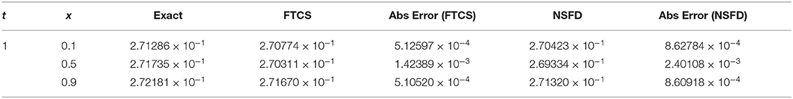
Table 2. A comparison between the exact and numerical solutions at some values of x for α = 1.0, β = 5.0, and γ = 0.01 at time t = 1.0.

TABLE 3

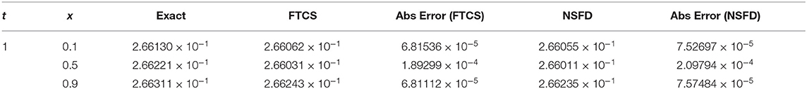
Table 3. A comparison between the exact and numerical solutions at some values of x for α = 1.0, β = 5.0, and γ = 0.01 at time t = 1.0.

FIGURE 2

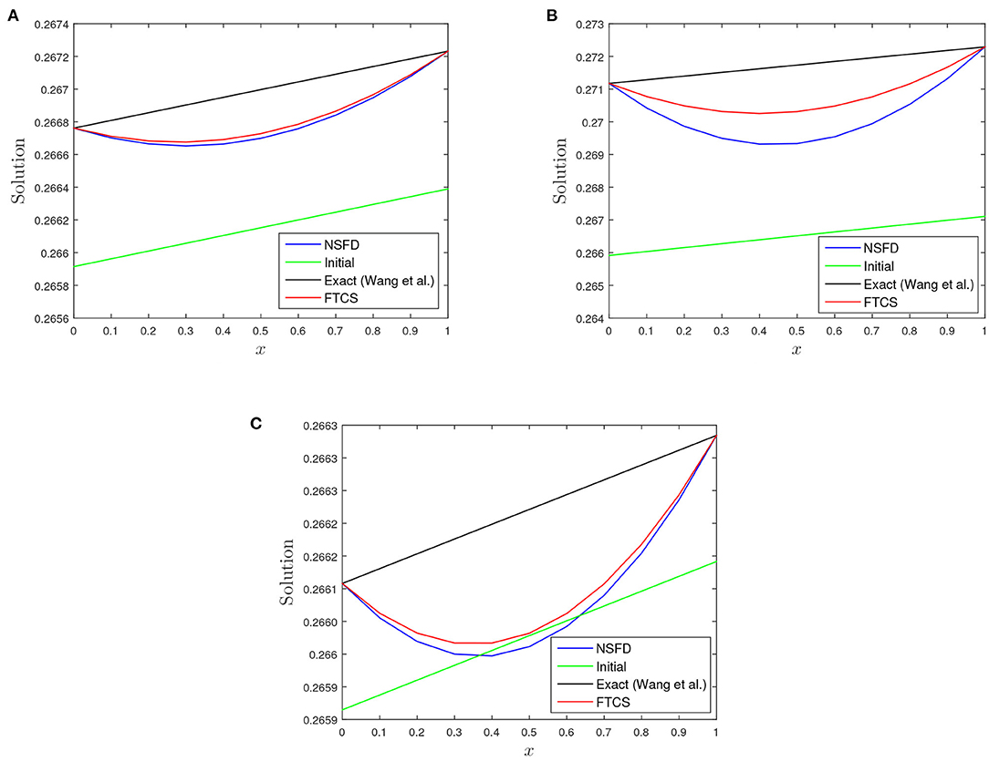
Figure 2. A plot of initial, numerical profiles, and profile from proposed solution [8] vs. x for the three test cases using FTCS and NSFD at t = 1.0 using h = 0.1 and k = 0.00125. (A) α = 1.0, β = 1.0, and γ = 0.01. (B) α = 1.0, β = 5.0, and γ = 0.01. (C) α = 5.0, β = 1.0, and γ = 0.01.

FIGURE 3

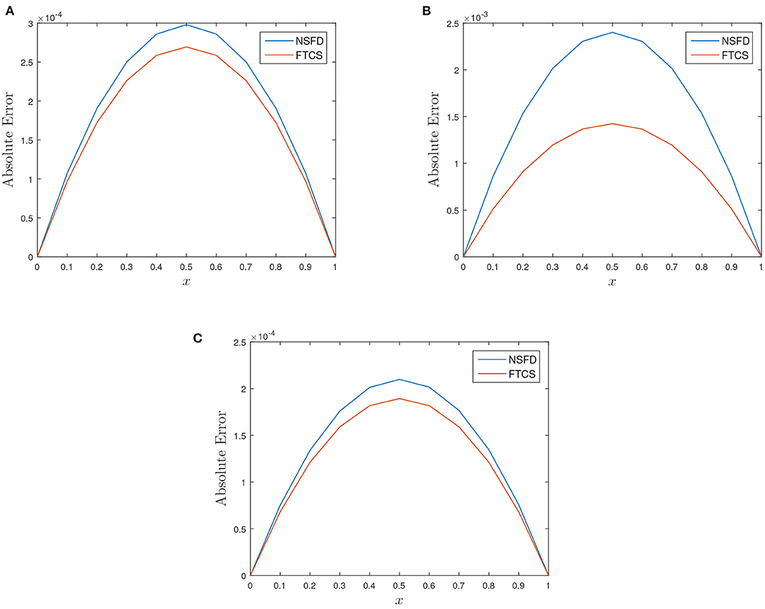
Figure 3. Plot of absolute error vs. x for the three test cases at t = 1.0 using h = 0.1 and k = 0.00125. (A) α = 1.0, β = 1.0, and γ = 0.01. (B) α = 1.0, β = 5.0, and γ = 0.01. (C) α = 5.0, β = 1.0, and γ = 0.01.

REMARK 4. There is always deviation in the numerical profiles (FTCS and NSFD) with the profile from proposed solution of Wang et al. [8] as depicted in Figure 1, despite performing grid refinement i.e., k → 0.

7. Numerical Results and Error Analysis Using proposed Solution From Deng

The results in this section are novel and are not taken from any reference.

Case 1: α = β = 1.0 and γ = 0.01.

Case 2: α = 1.0, β = 5.0, and γ = 0.01.

Case 3: α = 5.0, β = 1.0, and γ = 0.01.

Table 4 show the absolute error of the FTCS and NSFD schemes to be of order 10⁻⁷ while the relative error of both schemes is of order 10⁻⁶ − 10⁻⁷. When the reaction coefficient β dominates the advection coefficient α, we noticed a decline in the accuracy of both schemes (FTCS and NSFD) as the absolute errors increase to magnitude of order 10⁻⁵ − 10⁻⁷ and relative error to 10⁻⁶ and 10⁻⁵, respectively, as shown in Table 6. In Tables 5, 7, 9 show the rate of convergence as we perform grid refinement in time. Figures 4, 5 shed more light on the behaviour and performance of the FTCS and NSFD schemes with respect to the proposed solution of Deng [19].

TABLE 4

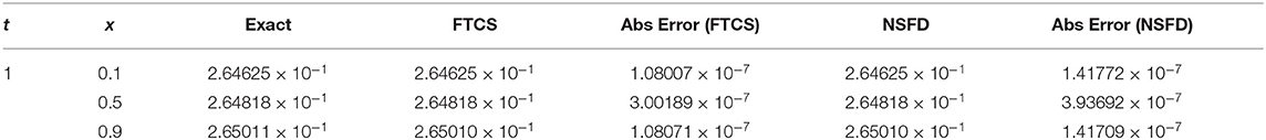
Table 4. A comparison between the exact and numerical solutions at some values of x for α = 1.0, β = 1.0, and γ = 0.01 at time t = 1.0.

TABLE 5

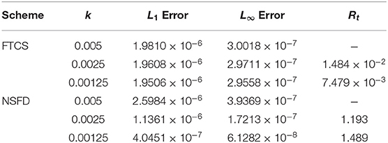
Table 5. L₁, L_∞ errors and rate of convergence (in time) for α = 1.0, β = 1.0, and γ = 0.01 (Case 1) at some different time-step size k with spatial mesh size h = 0.1 using FTCS and NSFD at t = 1.0.

TABLE 6

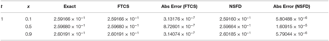
Table 6. A comparison between the exact and numerical solutions at some values of x for α = 1.0, β = 1.0, and γ = 0.01 at time t = 1.0.

TABLE 7

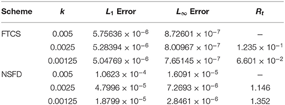
Table 7. L₁, L_∞ errors and rate of convergence (in time) for α = 1.0, β = 1.0, and γ = 0.01 (Case 2) at some different time-step size k with spatial mesh size h = 0.1 using FTCS and NSFD at t = 1.0.

FIGURE 4

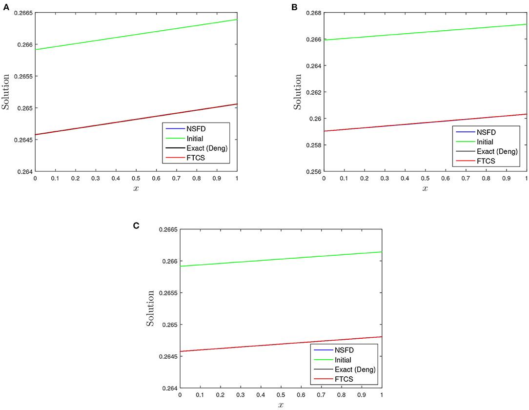
Figure 4. A plot of initial, numerical profiles, and profile from proposed solution [19] vs. x for the three test cases using FTCS and NSFD at t = 1.0 using h = 0.1 and k = 0.00125. (A) α = 1.0, β = 1.0, and γ = 0.01. (B) α = 1.0, β = 5.0, and γ = 0:01. (C) α = 5.0, β = 1.0, and γ = 0.01.

FIGURE 5

Figure 5. Plot of absolute error vs. x for the three test cases at t = 1.0 using h = 0.1 and k = 0.00125. (A) α = 1.0, β = 1.0, and γ = 0.01. (B) α = 1.0, β = 5.0, and γ = 0.01. (C) α = 5.0, β = 1.0, and γ = 0.01.

8. The Dynamics of a Travelling Wave by the Burgers-Huxley Equation

The Burgers-Huxley equation is a non linear PDE that exhibits many complex phenomena among which is the wave phenomenon. The proposed solutions are given in Equations

(9) and (10) both exhibit the dynamics of a travelling wave. A travelling wave is a wave that moves in a certain direction while maintaining a stable form. In this section, we show the travelling wave dynamics of the Burgers-Huxley equation using the proposed solution by Deng [19] and behaviour of the approximate solutions by looking at Equation (7) in an extended domain for the spatial variable x ∈ [−100, 100] and t ∈ [0, 1]. The plots are displayed in Figure 6.

FIGURE 6

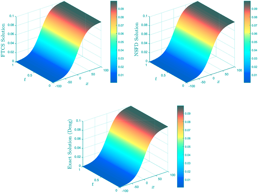
Figure 6. 3D plots of solution vs. t vs. x using FTCS, NSFD, and proposed solution [19] for α = 1, β = 1, δ = 1.0, and γ = 0.1 using k = 0.005 and h = 0.1.

9. Conclusion

In this work, we examined the two proposed solutions provided by Wang et al. [8] and Deng [19] for the generalised Burgers-Huxley equation. The FTCS and NSFD schemes are designed to approximate the solution of the generalised Burgers-Huxley equation. The numerical estimation tools of absolute error, relative error, and rate of convergence serve as the means of benchmarking the two proposed solutions. We observed that despite the consistency of the two (FTCS and NSFD) finite difference schemes and working within their region of stability, the results deviate from the proposed solution from Wang et al. [8] upon grid refinements. This directly has a greater impact on its error analysis as shown in Figure 1 and Tables 1–3. This anomalous behaviour was not experienced using the proposed solution of Deng [19] as seen in Figure 3 and Tables 4–9. In conclusion, the proposed solution of Wang et al. [8] indeed contains a minor error while the solution provided by Deng [19] is the true exact solution for the generalised Burgers-Huxley equation for the initial conditions given by Equation (8). In our future work, we will consider an application in microfluidic, microfluidics deals with the flow of fluids and suspensions in channels of sub-millimetre-sized cross-sections under the influence of external forces. In these instances, viscosity dominates over inertia, ensuring the absence of turbulence and the appearance of regular and predictable laminar flow streams, which implies an exceptional spatial and temporal control of solutes. The equation modelling microfluidics is as follows [30]:

$\begin{array}{ll}\{\begin{array}{l}\nabla ·u=0,\\ \rho {\displaystyle (\frac{\partial u}{\partial t}+(u·\nabla )u)}=-\nabla P+\eta {\nabla }^{2}u+\rho g& \end{array}& (45)\end{array}$

we will approach the set of partial differential equations given in Equation (45) using FTCS, NSFD, and possibly other methods.

TABLE 8

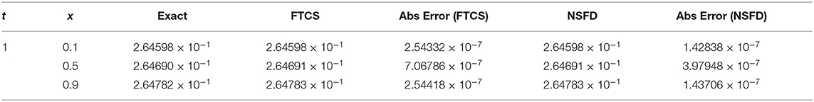
Table 8. A comparison between the exact and numerical solutions at some values of x for α = 1.0, β = 1.0, and γ = 0.01 at time t = 1.0.

TABLE 9

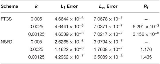
Table 9. L₁, L_∞ errors and rate of convergence (in time) for α = 1.0, β = 1.0, and γ = 0.01 (Case 3) at some different time-step size k with spatial mesh size h = 0.1 using FTCS and NSFD at t = 1.0.

Author Contributions

The plan of the paper was sent by AA, writing up was done by both authors. YT carried out the computations and analysis of the methods under the supervision of AA. AA and YT agree to be accountable for the content of the work.

Funding

YT acknowledges the support received from the Department of Mathematics and Applied Mathematics of the Nelson Mandela University which ensured that the author is registered for his Ph.D. study at the University for three years.

Conflict of Interest

The authors declare that the research was conducted in the absence of any commercial or financial relationships that could be construed as a potential conflict of interest.

Publisher's Note

All claims expressed in this article are solely those of the authors and do not necessarily represent those of their affiliated organizations, or those of the publisher, the editors and the reviewers. Any product that may be evaluated in this article, or claim that may be made by its manufacturer, is not guaranteed or endorsed by the publisher.

Acknowledgments

The authors are grateful to the two reviewers who provided feedback which allowed us to improve content and presentation of the paper considerably.

References

1. Adekanye O. The Construction of Nonstandard Finite Difference Schemes for dynamiCal Systems. Washington, DC: Howard University; (2017).

Google Scholar

2. Burgers JM. A mathematical model illustrating the theory of turbulence. Adv Appl Mech. (1948) 1:171–99. doi: 10.1016/S0065-2156(08)70100-5

CrossRef Full Text | Google Scholar

3. Abazari R, Borhanifar A. Numerical study of the solution of the Burgers and coupled Burgers equations by a differential transformation method. Comput Math Appl. (2010) 59:2711–22. doi: 10.1016/j.camwa.2010.01.039

CrossRef Full Text | Google Scholar

4. Mukundan V, Awasthi A. Linearized implicit numerical method for burgers' equation. Nonlinear Eng. (2016) 5:0031. doi: 10.1515/nleng-2016-0031

CrossRef Full Text | Google Scholar

5. Hodgkin AL, Huxley AF. A quantitative description of membrane current and its application to conduction and excitation in nerve. J Physiol. (1952) 117:500–44. doi: 10.1113/jphysiol.1952.sp004764

PubMed Abstract | CrossRef Full Text | Google Scholar

6. FitzHugh R. Impulses and physiological states in theoretical models of nerve membrane. Biophys J. (1961) 1:445–66. doi: 10.1016/S0006-3495(61)86902-6

PubMed Abstract | CrossRef Full Text | Google Scholar

7. Nagumo J, Arimoto S, Yoshizawa S. An active pulse transmission line simulating nerve axon. Proc IRE. (1962) 50:2061–70. doi: 10.1109/JRPROC.1962.288235

PubMed Abstract | CrossRef Full Text | Google Scholar

8. Wang XY, Zhu ZS, Lu YK. Solitary wave solutions of the generalized Burgers-Huxley equation. J Phys A. (1990) 23:271–4. doi: 10.1088/0305-4470/23/3/011

CrossRef Full Text | Google Scholar

9. Ismail HNA, Raslan K, Abd Rabboh AA. Adomian decomposition method for Burgers-Huxley and Burgers–Fisher equations. Appl Math Comput. (2004) 1:291–301. doi: 10.1016/j.amc.2003.10.050

CrossRef Full Text | Google Scholar

10. Batiha B, Noorani MSM, Hashim I. Application of variational iteration method to the generalized Burgers-Huxley equation. Chaos Solitons Fractals. (2008) 36:660–3. doi: 10.1016/j.chaos.2006.06.080

CrossRef Full Text | Google Scholar

11. Sari M, Gurarslan G. Numerical solutions of the generalized burgers-huxley equation by a differential quadrature method. Math Problems Eng. (2009) 2009:370765. doi: 10.1155/2009/370765

CrossRef Full Text | Google Scholar

12. Biazar J, Mohammadi F. Application of differential transform method to the generalized Burgers-Huxley Equation. Appl Appl Math. (2010) 5:629–43.

Google Scholar

13. Bratsos AG. A fourth order improved numerical scheme for the generalized burgers-Huxley Equation. Am J Comput Math. (2011) 1:660–3. doi: 10.4236/ajcm.2011.13017

CrossRef Full Text | Google Scholar

14. Ray SS, Gupta AK. Comparative analysis of variational iteration method and Haar wavelet method for the numerical solutions of Burgers-Huxley and Huxley equations. J Math Chem. (2014) 52:1066–80. doi: 10.1007/s10910-014-0327-z

CrossRef Full Text | Google Scholar

15. Singh BK, Arora G, Singh MK. A numerical scheme for the generalized Burgers-Huxley equation. J Egypt Math Soc. (2016) 24:629–837. doi: 10.1016/j.joems.2015.11.003

CrossRef Full Text | Google Scholar

16. Zibaei M, Zeinadini S, Namjoo M. Numerical solutions of Burgers-Huxley equation by exact finite difference and NSFD schemes. J Diff Equat Appl. (2016) 22:1098–113. doi: 10.1080/10236198.2016.1173687

CrossRef Full Text | Google Scholar

17. Verma KA, Kayenat S. An efficient Mickens' type NSFD scheme for the generalized Burgers Huxley equation. J Diff Equat Appl. (2020) 26:1213–46. doi: 10.1080/10236198.2020.1812594

CrossRef Full Text | Google Scholar

18. Cicek Y, Korkut S. Numerical solution of generalized burgers-huxley equation by lie-trotter splitting method. Numer Anal Appl. (2021) 14:90–102. doi: 10.1134/S1995423921010080

CrossRef Full Text | Google Scholar

19. Deng X. Travelling wave solutions for the generalized Burgers-Huxley equation. Appl Math Comput. (2008) 204:733–7. doi: 10.1016/j.amc.2008.07.020

CrossRef Full Text | Google Scholar

20. Macías-Díaz JE. A modified exponential method that preserves structural properties of the solutions of the Burgers-Huxley equation. Int J Comput Math. (2018) 95:3–19. doi: 10.1080/00207160.2017.1377339

CrossRef Full Text | Google Scholar

21. Ervin VJ, Macías-Díaz JE, Ruiz-Ramírez J. A positive and bounded finite element approximation of the generalized Burgers-Huxley equation. J Math Anal Appl. (2015) 424:1143–60. doi: 10.1016/j.jmaa.2014.11.047

CrossRef Full Text | Google Scholar

22. Nourazar SS, Soori M, Nazari-Golshan A. On the exact solution of burgers-huxley equation using the homotopy perturbation method. J Appl Math Phys. (2015) 95:285–94. doi: 10.4236/jamp.2015.33042

CrossRef Full Text | Google Scholar

23. Hadamard J. Sur les problèmes aux dérivées partielles et leur signification physique. Bull Univ Princeton. (1902) 13:49–52.

Google Scholar

24. Mohan MT, Khan A. On the generalized Burgers-Huxley equation: existence, uniqueness, regularity, global attractors and numerical studies. Discrete Continuous Dyn Syst B. (2021) 26:3943–88. doi: 10.3934/dcdsb.2020270

CrossRef Full Text | Google Scholar

25. Appadu AR, Tijani YO, Aderogba AA. On the performance of some NSFD methods for a 2-D generalized Burgers-Huxley equation. J Diff Equat Appl. (2021) 27:1537–73. doi: 10.1080/10236198.2021.1999433

CrossRef Full Text | Google Scholar

26. Prieto FU, Muñoz JJB, Corvinos LG. Application of the generalized finite difference method to solve the advection–diffusion equation. J Comput Appl Math. (2011) 235:1849–55. doi: 10.1016/j.cam.2010.05.026

CrossRef Full Text | Google Scholar

27. Mickens RE. Application of Nonstandard Finite Difference Scheme. Singapore: World Scientific (2000).

Google Scholar

28. Appadu AR, İnan B, Tijani YO. Comparative study of some numerical methods for the Burgers-Huxley equation. Symmetry. (2019) 11:1333. doi: 10.3390/sym11111333

CrossRef Full Text | Google Scholar

29. Appadu AR, Tijani YO, Munyakazi J. Computational study of some numerical methods for the generalized Burgers-Huxley equation. In: Awasthi A, John SJ, Panda S, editors. Computational Sciences-Modelling, Computing and Soft Computing. CSMCS Communications in Computer and Information Science, Vol. 1345. Singapore: Springer (2020).

Google Scholar

30. Bruus H. Governing equations in microfluidics. Microscale Acoustofluidics. (2014) 1–28. doi: 10.1039/9781849737067-00001

CrossRef Full Text | Google Scholar