The Mathematics of Smoothed Particle Hydrodynamics (SPH) Consistency

1 Introduction

The basic form of Smoothed Particle Hydrodynamics (SPH) was introduced more than 40 years ago by Gingold and Monaghan [1] and Lucy [2] for solving the equations of fluid dynamics in the context of astrophysical flows. Since then, SPH has become a popular numerical method due to its countless applications to the study of a great variety of astrophysical processes along with its ever-increasing applications to fluid and solid mechanics, magnetohydrodynamics, cosmology, geophysics, engineering, health sciences, and computer-generated animations, among others.

SPH is a Lagrangian scheme that is based on particle interpolation to compute smooth field variables. Such particles¹ act as control masses and carry all physical properties of the system to be simulated. Because of its Lagrangian nature, SPH has clear advantages over traditional mesh-dependent Eulerian methods. For example, it does not suffer from mesh distortions that affect the numerical accuracy in simulations of large material deformations. Most importantly, advection is performed exactly and therefore material history information can be tracked free of numerical diffusion. While these advantages cast SPH as a potential method for solving many kinds of problems, the method in its classical flavor suffers from slow numerical convergence due to loss of particle consistency, which has motivated in the last 20 years different modifications and corrections to the original formulation [3–13]. Consistency is a mathematical concept that is related to how well the discrete equations approximate the exact differential equations [14]. In other words, it is a measure of the local truncation error carried by the numerical discretization of the governing equations. In SPH, consistency is always approached under the assumption that the numerically approximated function is sufficiently smooth between particles. This is a quite acceptable assumption because information of the function is not available at scales smaller than the interparticle separation distances. Unlike traditional grid-based methods, the SPH discretization is performed in two separate steps: the kernel approximation and the particle approximation. Therefore, any error analysis will involve a two step process. In particular, the loss of particle consistency in standard SPH arises from the particle discretization procedure and the discrepancy that emerges between the kernel and the particle approximations is referred to as particle inconsistency [6]. In general three different sources of particle inconsistency have been identified, namely: truncation of the kernel support due to the presence of a physical boundary, irregular distributions of particles, and spatially varying smoothing lengths in adaptive calculations [6]. In particular, the problem of particle inconsistency in the presence of two-dimensional irregular boundaries was revised more recently by Fourtakas et al. [15], where C⁰ consistency is restored by discretizing the wall by means of a set of virtual particles.

Early corrective strategies to restore particle consistency were first advanced by Li and Liu [16] and Liu et al. [17], where the kernel function is modified to ensure that polynomial functions are exactly interpolated up to a given degree. Based on a variational formulation of SPH, Bonet and Lok [18] proposed kernel gradient corrections to allow exact evaluation of the gradient of a linear function, while Liu et al. [19] proposed a reconstruction approach of the kernel function that obeys the consistency conditions of SPH in continuous form (i.e., the conditions that the moments of the kernel must satisfy to guarantee completeness). However, this latter approach was quickly put aside because the reconstruction procedure may result in partially negative, non-symmetric, and non-monotonically decreasing smoothing functions, compromising the stability properties of SPH. More stable schemes for restoring particle consistency rely on Taylor series expansions of the kernel approximation of a function and its spatial derivatives. For example, if m derivatives are retained in the series expansion, then the resulting kernel and particle approximations will have (m + 1)th-order accuracy, or C^m consistency. Based on this observation, Chen et al. [3, 4] proposed the Corrective Smoothed Particle Method (CSPM), which is obtained by ignoring all derivatives in the expansion of the function and retaining only first-order terms in the expansions of the derivatives of the function. This method restores C¹ kernel consistency everywhere except at the boundaries, where the kernel consistency drops to C⁰. However, C¹ particle consistency is restored only for uniformly distributed particles, while at the boundaries and for irregular particle distributions the particle approximation is only C⁰-consistent. The CSPM approximations obtained this way have the same form of a Shepard’s interpolation for the function and its gradient [20]. Improvements to the CSPM approach were further introduced by Liu and Liu [6]. Their FPM scheme was designed to restore C¹ particle consistency everywhere by retaining first-order terms in the Taylor series expansions for the function and its derivatives and allowing the simultaneous solution of the resulting set of linear equations. An even better approach was proposed by Zhang and Batra [5] (their MSPH scheme) by retaining up to second-order terms in the Taylor series expansions. This method was claimed to restore C² particle consistency (i.e., third-order convergence rates) for the function and C¹ particle consistency for the first-order derivatives. However, a drawback of this approach is that when adding higher-order derivatives to the Taylor series expansions, the number of algebraic linear equations that must be solved simultaneously increases. Since the solution involves a matrix inversion, this not only affects the computational efficiency when large matrices are tried, but also compromises the stability of the overall scheme in situations where the matrix becomes ill-conditioned. A FPM-like scheme, which is free of kernel gradients and results in a symmetric corrective matrix was introduced by Huang et al. [10].

Alternative formulations to methods relying on Taylor series expansions were also reported in the literature. For example, Ferrand et al. [21, 22] proposed an approach based on a Shepard renormalization of the boundary integrals in the kernel approximation of the spatial derivatives in order to restore C⁰ consistency close to physical wall boundaries in weakly compressible SPH calculations, while Macià et al. [23] extended the scheme for incompressible SPH formulations, where a Poisson equation is solved for the pressure field, and performed a consistency analysis. A consistent Shepard interpolation for both the kernel and the kernel gradient was recently introduced by Reinhardt et al. [24] for applications to fluid animation. These authors noted that in the classical Shepard interpolation scheme the correction factors and the fluid quantities are calculated using different kernels, i.e., the uncorrected kernel is used for the correction factors, while the corrected kernel is employed in the calculation of all fluid quantities. This results in an inconsistent scheme since new errors are introduced, which may distort the density field even more than in simulations without a kernel correction. In this formulation C⁰ consistency is restored by correcting the volumes of source and neighboring particles simultaneously. A further recent contribution to SPH consistency from the computer graphics and animation community consisted in the formulation of a physically consistent implicit viscosity solver for incompressible and highly-viscous flows [25]. This method produces realistic animations of very complex flows as, for example, the buckling and rope coiling effects observed in nature when a thin stream of honey or caramel flows from a spoon. Such improvements are not only useful for animation purposes, but also for other science and engineering applications. Improved simulations of highly-viscous free-surface flows were recently reported by Kondo et al. [26]. A completely different scheme based on a piecewise high-order Moving-Least-Squares WENO reconstruction and the use of Riemann solvers was presented by Avesani et al. [27]. In particular, this latter approach was found to improve the accuracy and stability of SPH in the presence of sharp discontinuities.

As was first realized by Rasio [28] and then analyzed by Zhu et al. [13], a new source of inconsistency is due to the use of small numbers of neighbors per particle in simulations with compactly supported kernels. A formal derivation of the error carried by the SPH interpolation by Sigalotti et al. [29] has shown that the inconsistency is removed by increasing the number of neighbors. This was thereafter tested in the astrophysical context with reasonably good results [30, 31]. In this approach no corrections to the SPH discretization are required and full particle consistency is restored in the asymptotic limit N → ∞, h → 0, and n_neigh → ∞ with n_neigh/N → 0, where N is the total number of particles, h is the smoothing length, and n_neigh is the number of neighbors within the kernel support. Unlike most modern applications of SPH, Zhu et al. [13] demonstrated that C⁰ particle consistency can be achieved when working with a large number of neighbors and correspondingly small values of h. This result is consistent with the analysis performed by Read et al. [32], who found that working with a small number of neighbors, as it is common practice in SPH simulations, particle consistency is lost due to irreducible zeroth-order errors that will appear even though N → ∞ and h → 0. In spite of these improvements, the issue of convergence in a rigorous mathematical sense and its relation to the conservation properties have not been well understood. However, encouraging preliminary steps in this line were first put forward by Di Lisio et al. [33], Moussa and Vila [34], Quinlan et al. [35], Vignjevic et al. [36], Vaughan et al. [37], Fatehi and Manzari [38], and more recently by Sigalotti et al. [39], who developed an error analysis in n-dimensional space using the Poisson summation formula and derived for the first time the functional dependence of the error bounds on the SPH interpolation parameters, namely N, h, and n_neigh. In the following, an overview of the mathematical aspects of the SPH consistency will be given by focusing on the most recent advances. The paper is organized as follows. The standard SPH formulation along with the problem of particle inconsistency are briefly described in Section 2, while Section 3 deals with an overview of the most popular corrective schemes. Section 4 presents and discusses new insights and developments that have been made to improve the consistency of standard SPH. A brief discussion on the strategies that SPH practitioners must follow to achieve consistency in their applications is given in Section 5, while Section 6 contains the conclusions.

2 Conventional SPH Formulation

The foundation of SPH is interpolation theory. The starting point of the method lies on the Dirac sifting property

$f\left(\mathbf{x}\right)={\int }_{\mathrm{\Omega }}f\left({\mathbf{x}}^{\prime }\right)\delta \left(\mathbf{x}-{\mathbf{x}}^{\prime }\right)d^n{\mathbf{x}}^{\prime },(1)$

where f(x) is some smooth function defined in the domain $\mathrm{\Omega }\subseteq {\mathbb{R}}^n$ and evaluated at the generic point x ∈ Ω, δ(x − x′) is the Dirac delta distribution, and n denotes the spatial dimension (n = 1, 2, or 3).

2.1 Kernel Approximation

The kernel approximation is obtained by substituting the Dirac delta distribution by an interpolation function such that

$⟨f\left(\mathbf{x}\right)⟩={\int }_{\mathrm{\Omega }}f\left({\mathbf{x}}^{\prime }\right)W\left(\parallel \mathbf{x}-{\mathbf{x}}^{\prime }\parallel ,h\right)d^n{\mathbf{x}}^{\prime },(2)$

where ⟨f(x)⟩ is the smoothed estimate of f(x), W = W(∥x − x′ ∥, h) is the interpolation or smoothing kernel function, and h is the smoothing length. In general, W is a bell-shaped function defined such that: (1) it must satisfy the normalization condition

$M_0={\int }_{\mathrm{\Omega }}W\left(\parallel \mathbf{x}-{\mathbf{x}}^{\prime }\parallel ,h\right)d^n{\mathbf{x}}^{\prime }=1,(3)$

2) it must equal the Dirac delta distribution in the limit h → 0, 3) it must be positive definite, 4) it must be an even function such that W(∥x − x′ ∥, h) = W(∥x′ − x ∥, h), and 5) it must be a monotonically decreasing function. In addition, modern applications of SPH employ kernels of compact support for which W = 0 except within a sphere of radius kh from the center x, where k is some integer that depends on the kernel. Hence, W = 0 for ∥x − x′ ∥≥ kh. If f(x′) in the integrand of Eq. 2 is expanded in Taylor series about x, the kernel approximation becomes [39].

$⟨f\left(\mathbf{x}\right)⟩=f\left(\mathbf{x}\right)+\sum _{l=1}^{\infty }\frac{1}{l!}{\nabla }^{\left(l\right)}f\left(\mathbf{x}\right)\colon\colon \dots :{\int }_{\mathrm{\Omega }}{\left({\mathbf{x}}^{\prime }-\mathbf{x}\right)}^{l}W\left(\parallel \mathbf{x}-{\mathbf{x}}^{\prime }\parallel ,h\right)d^n{\mathbf{x}}^{\prime },(4)$

where ∇^(l) is the product of the ∇ operator l times with respect to coordinate x, the symbol ::…: is used to denote the lth-order inner product, and (x′ −x)^l is a tensor of rank l. It is clear from Eq. 4 that ⟨f(x)⟩ → f(x) only if the family of consistency relations are satisfied for the moments of the kernel

${\mathbf{M}}_l={\int }_{\mathrm{\Omega }}{\left({\mathbf{x}}^{\prime }-\mathbf{x}\right)}^{l}W\left(\parallel \mathbf{x}-{\mathbf{x}}^{\prime }\parallel ,h\right)d^n{\mathbf{x}}^{\prime }={\mathbf{0}}^{\left(l\right)},(5)$

for l = 1, 2, … , where 0⁽¹⁾ = (0, 0, 0) is the null vector and 0^(l) is the null tensor of rank l. C⁰ kernel consistency is always guaranteed by virtue of the normalization condition Eq. 3, while C¹ kernel consistency is automatically ensured because for l = 1 Eq. 5 is always satisfied due to the symmetry of the kernel. The same is also true for all odd values of l. Therefore, only for l even the above integrals do not necessarily vanish and for l = 2 a second-order error follows for the estimate of the function. Therefore, C² kernel consistency is not achieved by the kernel approximation unless a higher-order kernel is used for which M₂ = 0⁽²⁾ [40]. Similar expressions to Eqs 2, 5 for the estimate of the gradient and its moments can be derived as

$⟨\nabla f\left(\mathbf{x}\right)⟩={\int }_{\mathrm{\Omega }}f\left({\mathbf{x}}^{\prime }\right)\nabla W\left(\parallel \mathbf{x}-{\mathbf{x}}^{\prime }\parallel ,h\right)d^n{\mathbf{x}}^{\prime },(6)$

and

$\begin{array}{ccc}\hfill {\mathbf{M}}_0^{\prime }& =\hfill & {\int }_{\mathrm{\Omega }}\nabla W\left(\parallel \mathbf{x}-{\mathbf{x}}^{\prime }\parallel ,h\right)d^n{\mathbf{x}}^{\prime }={\mathbf{0}}^{\left(1\right)},\hfill \\ \hfill {\mathbf{M}}_1^{\prime }& =\hfill & {\int }_{\mathrm{\Omega }}\left({\mathbf{x}}^{\prime }-\mathbf{x}\right)\nabla W\left(\parallel \mathbf{x}-{\mathbf{x}}^{\prime }\parallel ,h\right)d^n{\mathbf{x}}^{\prime }=\mathbb{I},\hfill \\ \hfill {\mathbf{M}}_l^{\prime }& =\hfill & {\int }_{\mathrm{\Omega }}{\left({\mathbf{x}}^{\prime }-\mathbf{x}\right)}^l\nabla W\left(\parallel \mathbf{x}-{\mathbf{x}}^{\prime }\parallel ,h\right)d^n{\mathbf{x}}^{\prime }={\mathbf{0}}^{\left(l+1\right)},\hfill \end{array}(7)$

for l = 2, 3, … , where $\mathbb{I}$ is the unit tensor of second rank. Therefore, exact approximation to the gradient requires that the kernel consistency relations given by Eq. 7 are exactly fulfilled.

2.2 Particle Approximation

The SPH discretization makes reference to a set of Lagrangian particles which may, in general, be disordered as a consequence of their being convected with the fluid. The discretization is shown schematically in Figure 1, where the domain Ω is divided into N subdomains, Ω_k, within each of which lies a Lagrangian particle at point x_k chosen such that x_k ∈ Ω_k. It is common practice to define the boundaries of the Lagrangian subdomains, i.e., ∂Ω_k, such that their masses remain constant. The kernel support is termed Ω_s, which may be a circle in two-dimensions or a sphere in three-dimensions, and is centered at the observation point x_a. Thus, the numerical integration is performed over the intersection set between Ω_s and the finite model domain Ω. The elements of the intersection set are the neighbors around particle a (or subdomain Ω_a).

FIGURE 1

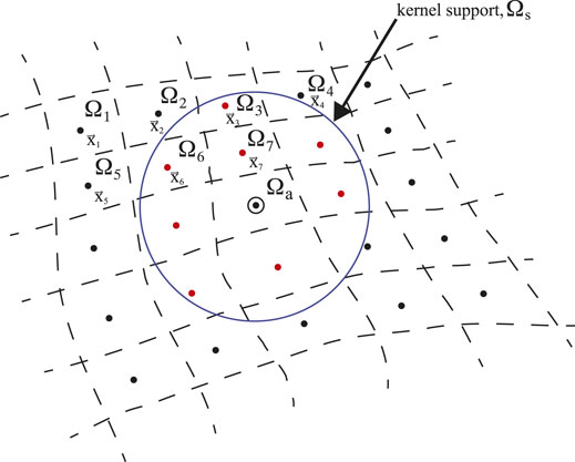
FIGURE 1. Schematic of the SPH discretization with a compactly supported kernel function.

Using the mean value theorem so that x_b ∈ Ω_b for each neighbor b of the observation particle a and denoting by V_b the volume of Ω_b, Eq. 2 in discretized form becomes

$f_a=⟨f\left({\mathbf{x}}_a\right)⟩=\sum _{b=1}^{n_{\text{neigh}}}{\int }_{{\mathrm{\Omega }}_b}f\left({\mathbf{x}}^{\prime }\right)W\left(\parallel {\mathbf{x}}_a-{\mathbf{x}}^{\prime }\parallel ,h\right)d^n{\mathbf{x}}^{\prime }\approx \sum _{b=1}^{n_{\text{neigh}}}f\left({\mathbf{x}}_b\right)W\left(\parallel {\mathbf{x}}_a-{\mathbf{x}}_b\parallel ,h\right)V_b,(8)$

where the last term in Eq. 8 is called the summation interpolant. From now on we will simplify the notation by setting W_ab = W(∥x_a − x_b ∥, h) and n_a = n_neigh for the number of neighbors of particle a, which should not be confused with the same letter used for the dimension. Here the subscript a is used to denote a generic observation particle and the subscript b is used to denote its neighbors. Therefore, in simplified form the particle estimate of function f(x) at the observation point x_a becomes

$f_a=\sum _{b=1}^{n_a}{f}_b{W}_{ab}{V}_b=\sum _{b\in {\mathcal{N}}_a}{f}_b{W}_{ab}{V}_b,(9)$

as it is traditionally written in the SPH literature [41–44]. Here ${\mathcal{N}}_a=\{\mathrm{1,2},\dots ,n_a\}$ is the set of all neighbors of particle a and the second summation stresses the fact that subscript b takes only values pertaining to this set. In general, all particles have the same number of neighbors so that the number of elements of ${\mathcal{N}}_a$ is always the same (i.e., n = n_a). In actual SPH applications it is customary to replace the particle volume V_b by the ratio m_b/ρ_b, where m_b and ρ_b are the mass and density of particle b, respectively. For quasi-ordered particles following a low-discrepancy sequence, Fulk [45] proved that the SPH approximation (9) is consistent with the identity operator, If(x) = f(x), under the uniform norm

$\parallel Sf-If{\parallel }_{\infty }=\parallel Kf-If+Sf-Kf{\parallel }_{\infty }\le \parallel Kf-If{\parallel }_{\infty }+\parallel Sf-Kf{\parallel }_{\infty },(10)$

only if V_b = m_b/ρ_b, where If = f(x_a) is the exact value of the function evaluated at point x_a, while Kf = ⟨f(x_a)⟩ and Sf = f_a are, respectively, the kernel and particle estimates of the function at x_a defined by Eqs 2, 9. In the limit of vanishing inter-particle distances ∥ Sf − Kf ∥_∞ → 0, whereas ∥ Kf − If ∥_∞ → 0 as h → 0. Therefore, it has always been common practice to write Eq. 9 as

$f_a=\sum _{b\in {\mathcal{N}}_a}{m}_b\frac{f_b}{{\rho }_b}{W}_{ab}.(11)$

Following similar steps, the particle approximation of Eq. 6 can be written as

${\left(\nabla f\right)}_a=\sum _{b\in {\mathcal{N}}_a}{m}_b\frac{f_b}{{\rho }_b}{\nabla }_a{W}_{ab}.(12)$

A better representation of the gradient, which vanishes exactly when the function is a constant, is given by [46]

${\left(\nabla f\right)}_a=\sum _{b\in {\mathcal{N}}_a}\frac{m_b}{{\rho }_b}\left(f_b-f_a\right){\nabla }_a{W}_{ab}.(13)$

Other alternative representations can be found in the literature guided by momentum conservation requirements [41, 42].

2.3 Particle Inconsistency

The SPH approximation given by Eq. 11 introduces two types of error. The first one comes from the kernel approximation which is ∝ h^m, where m is a small integer that depends on the order of completeness that is enforced. This error is independent of the particle distribution and for most commonly used kernels it contributes with a second-order term (i.e., m = 2). The second error originates from the discretization procedure and is a function of the number of neighbors, ϕ = ϕ(n), and depends on how they are actually distributed within Ω_s. It has long been conjectured that ϕ(n) ∝   log  n/n when the neighbors are quasi-ordered [46], while if they are randomly distributed then ϕ(n) ∝ n^−1/2 [13]. The dependence of the discretization error on n can be parameterized as ϕ(n) ∝ n^−p, where 1/2 ≤ p ≤ 1. Zhu et al. [13] noted that the reduction of the overall error would demand making h smaller and, at the same time, n larger so that the combined limit N → ∞, h → 0, and n → ∞, with n/N → 0, would be necessary to achieve full consistency. This limit was first noted by Rasio [28] using a simple analysis based on sound waves. From the matching between the smoothing and particle discretization errors, Zhu et al. [13] proposed the following power-law dependences of h and n on the total number of particles (N)

$h\propto N^{-1/\beta },n\propto N^{1-3/\beta },(14)$

where β − 3 + m/p. Thus, for m = 2 and a random distribution (p = 1/2), β − 7 and n ∝ N^0.57, while for quasi-ordered distributions (p = 1), β − 5 and n ∝ N^0.4. For an intermediate value of β(− 6), h ∝ N^−1/6 and n ∝ N^1/2. If higher-order kernels (m > 2) are chosen, a stronger scaling of n with N would be required. From a truncation error analysis of the SPH approximation of spatial derivatives in one dimension, Quinlan et al. [35] suggested that the SPH errors will decay as h² if h is reduced while maintaining Δ/h constant, where Δ is the inter-particle distance. If, on the other hand, Δ/h is reduced while maintaining h fixed, the error will also decrease, which is equivalent to increase the number of neighbors. Using the Euler equations, Read et al. [32] realized that the loss of particle consistency is due to the presence of h-independent, zeroth-order error terms that are irreducible even when N → ∞, h → 0, and n is maintained constant at the low values typically used in most SPH applications. They suggested as a convergence criterion that n must increase to ensure that ϕ(n) shrinks faster than the smoothing error (∝ h^m). A similar result was reported by Vaughan et al. [37], who found that if C⁰ consistency is not restored the error does not converge with h, whereas if C¹ consistency is achieved then the error goes as −$h^2$.

The claim of particle consistency based solely on the equivalence V_b → m_b/ρ_b is not sufficient because in general the conditions on the kernel moments given by Eqs 3, 5 are not fulfilled in discrete form, i.e.,

$\begin{array}{ccc}\hfill M_{0,a}& =\hfill & \sum _{b\in {\mathcal{N}}_a}\frac{m_b}{{\rho }_b}{W}_{ab}\ne 1,\hfill \end{array}(15)$

$\begin{array}{ccc}\hfill {\mathbf{M}}_{l,a}& =\hfill & \sum _{b\in {\mathcal{N}}_a}\frac{m_b}{{\rho }_b}{\left({\mathbf{x}}_b-{\mathbf{x}}_a\right)}^l{W}_{ab}\ne {\mathbf{0}}^{\left(l\right)},\hfill \end{array}(16)$

and similarly for the particle form of the integral conditions in Eq. 7 for the kernel gradient. The loss of C⁰ particle consistency is a clear manifestation of the violation of the discrete form of the probability function given by Eq. 15 even for regularly ordered particles because of noise errors that scale with n as −$n^{-1}$. In practical applications, as the particles are convected with the fluid, node disorder results in amplified noise, leading to loss of C⁰ consistency because of more severe deviations of the particle normalization condition from unity. Loss of C⁰ consistency also occurs when Ω_s is truncated by a physical boundary or when spatially and temporally adaptive kernels are employed [6].

2.4 Conservation Principles

The loss of particle consistency in fluid simulations may affect the fundamental principles of physics, such as the principles of conservation of mass, energy, linear momentum, and angular momentum. For most applications, the conservation of mass and linear momentum represents irreducible requirements. Restoring particle consistency is therefore important to guarantee local conservation because if a condition is satisfied locally everywhere within a domain, then it will be also satisfied globally.

Local and global mass conservation can be satisfied exactly by using Eq. 11 with f → ρ to evaluate the density provided that all particles with Lagrangian boundaries preserve their mass. As was demonstrated by Vignjevic et al. [36], if C⁰ particle consistency is achieved, then the homogeneity of space is not affected by the process of spatial discretization, which in turn has, as a consequence, the conservation of linear momentum. In other words, under C⁰ particle consistency the SPH interpolation becomes independent of rigid-body translations of the coordinates. To put this in mathematical form, let us first approximate the position vector x_a using Eq. 11

${\mathbf{x}}_a=\sum _{b\in {\mathcal{N}}_a}{\mathbf{x}}_b\frac{m_b}{{\rho }_b}{W}_{ab}.(17)$

The transformed coordinates x′ = x + Δx will then be estimated according to

${\mathbf{x}}_a^{\prime }=\sum _{b\in {\mathcal{N}}_a^{\prime }}{\mathbf{x}}_b^{\prime }\frac{m_b^{\prime }}{{\rho }_b^{\prime }}{W}_{ab}^{\prime },(18)$

where $W_{ab}^{\prime }=W(\parallel {\mathbf{x}}_a^{\prime }-{\mathbf{x}}_b^{\prime }\parallel ,h^{\prime })$, $m_b^{\prime }={\rho }_b^{\prime }{V}_b^{\prime }$, ${\mathcal{N}}_a^{\prime }=\{\mathrm{1,2},\dots ,n^{\prime }=n_a^{\prime }\}$, and n′ is the number of neighbors in the transformed support domain ${\mathrm{\Omega }}_s^{\prime }$ of radius kh′. Preservation of space homogeneity under uniform translations demands that ${\mathbf{x}}_a^{\prime }={\mathbf{x}}_a+⟨\mathrm{\Delta }\mathbf{x}⟩$, with ⟨Δx⟩ = Δx. Replacing ${\mathbf{x}}_b^{\prime }$ by x_b + Δx in Eq. 18 it is easy to show that

${\mathbf{x}}_a^{\prime }={\mathbf{x}}_a+\mathrm{\Delta }\mathbf{x}\sum _{b\in {\mathcal{N}}_a}\frac{m_b}{{\rho }_b}{W}_{ab}={\mathbf{x}}_a+\mathrm{\Delta }\mathbf{x}{M}_{0,a},(19)$

where we have made $m_b^{\prime }=m_b$, $W_{ab}^{\prime }=W_{ab}$, and n′ = n because under solid-body translations the coordinates of a point are independent of the translation of the coordinate axes. Therefore, Eq. 19 expresses that homogeneity of the discrete space is satisfied by the SPH interpolation only when the condition M_0,a = 1, i.e., only when C⁰ particle consistency is restored². Vignjevic et al. [36] also demonstrated that angular momentum conservation is exactly preserved only if the isotropy of space is not affected by the SPH interpolation. This is equivalent to demand that the SPH interpolation must be invariant under solid-body rotation of the coordinate axes. In order to simplify the mathematical operations, let us consider only small rotations so that the coordinates are transformed according to

${\mathbf{x}}^{\prime }=\mathbf{x}-d\mathbf{w}\times \mathbf{x}=\mathbf{x}-\mathbf{x}\cdot \nabla \left(d\mathbf{w}\times \mathbf{x}\right),(20)$

where dw is the differential rotation vector. Under solid-body rotation, the coordinates of a point are invariant with respect to a rotation of the coordinate axes and therefore [∇(dw ×x)]_a = ∇(dw ×x), or using the particle approximation given by Eq. 12

${\left[\nabla \left(d\mathbf{w}\times \mathbf{x}\right)\right]}_a=\sum _{b\in {\mathcal{N}}_a}\frac{m_b}{{\rho }_b}{\left(d\mathbf{w}\times \mathbf{x}\right)}_b{\nabla }_a{W}_{ab}=\nabla \left(d\mathbf{w}\times \mathbf{x}\right)\cdot \sum _{b\in {\mathcal{N}}_a}\frac{m_b}{{\rho }_b}{\mathbf{x}}_b{\nabla }_a{W}_{ab},(21)$

which implies that the first moment of the gradient given by Eq. 7 in discrete form must satisfy the condition

${\mathbf{M}}_1^{\prime }=\sum _{b\in {\mathcal{N}}_a}\frac{m_b}{{\rho }_b}{\mathbf{x}}_b{\nabla }_a{W}_{ab}=\mathbb{I},(22)$

in order to preserve the isotropy of the discrete space and conserve angular momentum. In summary, the particle approximation does not affect the conservation of linear and angular momentum provided that C⁰ and C¹ consistencies are restored for the function and its gradient. When thermal effects are important, energy conservation is ensured by the first law of thermodynamics from which an equation for either the internal energy or the enthalpy is derived. Rotational invariance using the more accurate representation given by Eq. 13 requires that, in addition to the condition represented by Eq. 22, the discrete zeroth moment of the kernel gradient, ${\mathbf{M}}_0^{\prime }$, must vanish.

3 Corrective SPH Schemes

As was outlined above, SPH particle inconsistency is a manifestation of the discrepancy between the spatially discretized equations and their corresponding kernel approximation in continuous form. Improvements on this drawback is therefore mandatory for SPH to become a robust and reliable simulation tool. Earlier approaches to restore particle consistency were based on kernel reconstruction techniques [19, 47, 48]. Although these methods can reproduce a polynomial function and its derivatives to any desired order, they can sometimes lead to reconstructed kernels that may be non-positive, not symmetric, and not monotonically decreasing, yielding inaccurate results. In addition, the computational effort for constructing higher-order reproducing kernel functions could be quite intensive. More robust and stable approaches rely on a Taylor series expansion of the function and its derivatives in the kernel estimate. In what follows the most popular methods based on Taylor series expansions will be briefly reviewed along with some alternative recent schemes.

3.1 The Corrective Smoothed Particle Method (CSPM)

The CSPM scheme was originally developed by Chen et al. [3, 4] as a corrective scheme for approximating a function and its derivatives. In this formulation, the conventional kernel estimate of a function is expressed in terms of its Taylor series expansion about an arbitrary point of its domain of definition. Expansion of the function f(x) about the point x_a up to second-order terms gives

$f\left(\mathbf{x}\right)=f\left({\mathbf{x}}_a\right)+\left({\mathbf{x}}_a-\mathbf{x}\right)\cdot \nabla f\left({\mathbf{x}}_a\right)+\frac{1}{2}\left({\mathbf{x}}_a-\mathbf{x}\right)\left({\mathbf{x}}_a-\mathbf{x}\right):\nabla \nabla f\left({\mathbf{x}}_a\right)+\mathcal{O}\left[{\left({\mathbf{x}}_a-\mathbf{x}\right)}^3\right].(23)$

Multiplying the above expression by the kernel function W_a = W(∥x_a − x ∥, h) and integrating over the domain volume V, the result is

${\int }_{V}f\left(\mathbf{x}\right)W_{a}dV=f\left({\mathbf{x}}_a\right){\int }_V{W}_{a}dV+\nabla f\left({\mathbf{x}}_a\right)\cdot {\int }_V\left(\mathbf{x}-{\mathbf{x}}_a\right)W_{a}dV+\cdots ,(24)$

which after solving for f(x_a) and neglecting all terms containing derivatives, the corrective kernel estimate of the function becomes

$f\left({\mathbf{x}}_a\right)=\frac{{\int }_{V}f\left(\mathbf{x}\right)W_{a}dV}{{\int }_V{W}_{a}dV},(25)$

which is identical to the Shepard kernel interpolation [20]. From now on, the angle brackets used to denote the kernel estimate of the function will be dropped for simplicity. The approximations for the derivatives are constructed the same way by multiplying Eq. 23 by ∇W_a for the first derivatives and by ∇∇W_a for the second derivatives and then integrating both expressions over the whole volume of the domain. Retaining terms up to first-order, the expansion for the first derivatives becomes

$\nabla f\left({\mathbf{x}}_a\right)\cdot {\int }_V\left(\mathbf{x}-{\mathbf{x}}_a\right)\nabla W_{a}dV={\int }_V\left[f\left(\mathbf{x}\right)-f\left({\mathbf{x}}_a\right)\right]\nabla W_{a}dV.(26)$

Similarly, retaining terms up to the second-order in the expansion for the second derivatives, the result is

$\begin{array}{ccc}\hfill \frac{1}{2}\nabla \nabla f\left({\mathbf{x}}_a\right):{\int }_V\left({\mathbf{x}}_a-\mathbf{x}\right)\left({\mathbf{x}}_a-\mathbf{x}\right)\nabla \nabla W_{a}dV& =\hfill & {\int }_V\left[f\left(\mathbf{x}\right)-f\left({\mathbf{x}}_a\right)\right]\nabla \nabla W_{a}dV\hfill \\ \hfill & -\hfill & \nabla f\left({\mathbf{x}}_a\right)\cdot {\int }_V\left(\mathbf{x}-{\mathbf{x}}_a\right)\nabla \nabla W_{a}dV.\hfill \end{array}(27)$

In three-space dimensions, Eqs 26, 27 represent two independent sets of three and six coupled equations, respectively. Due to the symmetry of W, the second term on the right-hand side of Eq. 24 vanishes identically for points that are far from the boundaries of the domain, implying that the estimate given by Eq. 25 is of second-order for unbounded domains. However, for points close to a boundary Eq. 25 is only a first-order approximation because the second term on the right-hand side of Eq. 23 no longer vanishes. The same holds for the kernel approximation of the derivatives. Therefore, the whole scheme achieves C¹ kernel consistency away from the boundaries and C⁰ kernel consistency for points near or on the boundary. For numerical work, the particle approximation of Eq. 25 is just

$f_a=\frac{1}{M_{0,a}}\sum _{b\in {\mathcal{N}}_a}\frac{m_b}{{\rho }_b}{f}_b{W}_{ab},(28)$

while the particle approximation of Eq. 26 for the corrective first-order derivatives can be written in terms of the linear matrix equation

${\mathbb{A}}_a\cdot {\mathbf{F}}_a^{\prime }={\mathbf{b}}_a,(29)$

where $\mathbb{A}$ is a 3 × 3 matrix, F′ is the vector solution whose elements are the three derivative components, and b is a column vector. Using index notation, these quantities are given by

$\begin{array}{ccc}\hfill A_{lm,a}& =\hfill & \sum _{b\in {\mathcal{N}}_a}\frac{m_b}{{\rho }_b}\left(x_b^l-x_a^l\right)\frac{\partial W_{ab}}{\partial x_a^m},\hfill \\ \hfill F_{l,a}^{\prime }& =\hfill & {\left(\frac{\partial f}{\partial x^l}\right)}_a,\hfill \\ \hfill b_{m,a}& =\hfill & \sum _{b\in {\mathcal{N}}_a}\frac{m_b}{{\rho }_b}\left(f_b-f_a\right)\frac{\partial W_{ab}}{\partial x_a^m},\hfill \end{array}(30)$

where in three dimensions l, m = 1, 2, and 3. Since the integral on the left-hand side of Eq. 27 is a tensor of rank four and the other two integrals on the right-hand side are of second rank, the six components of the second-order derivatives can be obtained by solving the linear equation

${\mathbb{B}}_a\cdot {\mathbf{F}}_a^{\prime \prime }={\mathbf{d}}_a,(31)$

where in index notation

$\begin{array}{ccc}\hfill B_{lksm,a}& =\hfill & \left(1-\frac{1}{2}{\delta }_{lk}\right)\sum _{b\in {\mathcal{N}}_a}\frac{m_b}{{\rho }_b}\left(x_b^l-x_a^l\right)\left(x_b^k-x_a^k\right)\frac{{\partial }^2{W}_{ab}}{\partial x_a^s\partial x_a^m},\hfill \\ \hfill F_{lk,a}^{\prime \prime }& =\hfill & {\left(\frac{{\partial }^{2}f}{\partial x^l\partial x^k}\right)}_a,\hfill \\ \hfill d_{lsm,a}& =\hfill & \sum _{b\in {\mathcal{N}}_a}\frac{m_b}{{\rho }_b}\left(f_b-f_a\right)\frac{{\partial }^2{W}_{ab}}{\partial x_a^s\partial x_a^m}-{\left(\frac{\partial f}{\partial x^l}\right)}_a\sum _{b\in {\mathcal{N}}_a}\frac{m_b}{{\rho }_b}\left(x_b^l-x_a^l\right)\frac{{\partial }^2{W}_{ab}}{\partial x_a^s\partial x_a^m},\hfill \end{array}(32)$

for l, k, s, m = 1, 2, and 3 in three dimensions. The solution of Eqs 29, 31 uniquely determine the particle estimate of the three components of the first-order derivatives and the six components of the second-order derivatives at the position of particle a.

3.2 The Finite Particle Method (FPM)

The FPM approach was proposed by Liu and Liu [6] as an improved extension of the CSPM method for the kernel and particle approximations of the function and its first derivatives. The main differences with the CSPM scheme is that terms up to second-order are retained in the expansion given by Eq. 24 for the kernel and particle approximations of both the function and its first-order derivatives and that the particle estimates of the function and its derivatives are solved simultaneously. Using Cartesian coordinates the problem reduces to solve a linear system of the form

$\mathbb{A}\cdot \left[\begin{array}{c}\hfill f\left({\mathbf{x}}_a\right)\hfill \\ \hfill {\left(\frac{\partial f\left(\mathbf{x}\right)}{\partial x}\right)}_a\hfill \\ \hfill {\left(\frac{\partial f\left(\mathbf{x}\right)}{\partial y}\right)}_a\hfill \\ \hfill {\left(\frac{\partial f\left(\mathbf{x}\right)}{\partial z}\right)}_a\hfill \end{array}\right]=\left[\begin{array}{c}\hfill {\int }_{V}f\left(\mathbf{x}\right)W_{a}dV\hfill \\ \hfill {\int }_{V}f\left(\mathbf{x}\right)\frac{\partial W_a}{\partial x}dV\hfill \\ \hfill {\int }_{V}f\left(\mathbf{x}\right)\frac{\partial W_a}{\partial y}dV\hfill \\ \hfill {\int }_{V}f\left(\mathbf{x}\right)\frac{\partial W_a}{\partial z}dV\hfill \end{array}\right],(33)$

where $\mathbb{A}$ is a 4 × 4 matrix, which in three dimensions looks like

$\mathbb{A}=\left[\begin{array}{cccc}\hfill {\int }_V{W}_{a}dV\hfill & \hfill {\int }_V\left(x-x_a\right)W_{a}dV\hfill & \hfill {\int }_V\left(y-y_a\right)W_{a}dV\hfill & \hfill {\int }_V\left(z-z_a\right)W_{a}dV\hfill \\ \hfill {\int }_V\frac{\partial W_a}{\partial x}dV\hfill & \hfill {\int }_V\left(x-x_a\right)\frac{\partial W_a}{\partial x}dV\hfill & \hfill {\int }_V\left(y-y_a\right)\frac{\partial W_a}{\partial x}dV\hfill & \hfill {\int }_V\left(z-z_a\right)\frac{\partial W_a}{\partial x}dV\hfill \\ \hfill {\int }_V\frac{\partial W_a}{\partial y}dV\hfill & \hfill {\int }_V\left(x-x_a\right)\frac{\partial W_a}{\partial y}dV\hfill & \hfill {\int }_V\left(y-y_a\right)\frac{\partial W_a}{\partial y}dV\hfill & \hfill {\int }_V\left(z-z_a\right)\frac{\partial W_a}{\partial y}dV\hfill \\ \hfill {\int }_V\frac{\partial W_a}{\partial z}dV\hfill & \hfill {\int }_V\left(x-x_a\right)\frac{\partial W_a}{\partial z}dV\hfill & \hfill {\int }_V\left(y-y_a\right)\frac{\partial W_a}{\partial z}dV\hfill & \hfill {\int }_V\left(z-z_a\right)\frac{\partial W_a}{\partial z}dV\hfill \end{array}\right].(34)$

In discrete form, the solution vector containing the particle estimate of the function and its first derivatives is given by

$\left[\begin{array}{c}\hfill f_a\hfill \\ \hfill {\left(\frac{\partial f}{\partial x}\right)}_a\hfill \\ \hfill {\left(\frac{\partial f}{\partial y}\right)}_a\hfill \\ \hfill {\left(\frac{\partial f}{\partial z}\right)}_a\hfill \end{array}\right]={\mathbb{A}}_a^{-1}\cdot \left[\begin{array}{c}\hfill \sum _{b\in {\mathcal{N}}_a}\frac{m_b}{{\rho }_b}{f}_b{W}_a\hfill \\ \hfill \sum _{b\in {\mathcal{N}}_a}\frac{m_b}{{\rho }_b}{f}_b\frac{\partial W_a}{\partial x_a}\hfill \\ \hfill \sum _{b\in {\mathcal{N}}_a}\frac{m_b}{{\rho }_b}{f}_b\frac{\partial W_a}{\partial y_a}\hfill \\ \hfill \sum _{b\in {\mathcal{N}}_a}\frac{m_b}{{\rho }_b}{f}_b\frac{\partial W_a}{\partial z_a}\hfill \end{array}\right],(35)$

where

${\mathbb{A}}_a^{-1}={\left[\begin{array}{cccc}\hfill \sum _{b\in {\mathcal{N}}_a}\frac{m_b}{{\rho }_b}{W}_a\hfill & \hfill \sum _{b\in {\mathcal{N}}_a}\frac{m_b}{{\rho }_b}{x}_{ba}{W}_{ab}\hfill & \hfill \sum _{b\in {\mathcal{N}}_a}\frac{m_b}{{\rho }_b}{y}_{ba}{W}_{ab}\hfill & \hfill \sum _{b\in {\mathcal{N}}_a}\frac{m_b}{{\rho }_b}{z}_{ba}{W}_{ab}\hfill \\ \hfill \sum _{b\in {\mathcal{N}}_a}\frac{m_b}{{\rho }_b}\frac{\partial W_{ab}}{\partial x_a}\hfill & \hfill \sum _{b\in {\mathcal{N}}_a}\frac{m_b}{{\rho }_b}{x}_{ba}\frac{\partial W_{ab}}{\partial x_a}\hfill & \hfill \sum _{b\in {\mathcal{N}}_a}\frac{m_b}{{\rho }_b}{y}_{ba}\frac{\partial W_{ab}}{\partial x_a}\hfill & \hfill \sum _{b\in {\mathcal{N}}_a}\frac{m_b}{{\rho }_b}{z}_{ba}\frac{\partial W_{ab}}{\partial x_a}\hfill \\ \hfill \sum _{b\in {\mathcal{N}}_a}\frac{m_b}{{\rho }_b}\frac{\partial W_{ab}}{\partial y_a}\hfill & \hfill \sum _{b\in {\mathcal{N}}_a}\frac{m_b}{{\rho }_b}{x}_{ba}\frac{\partial W_{ab}}{\partial y_a}\hfill & \hfill \sum _{b\in {\mathcal{N}}_a}\frac{m_b}{{\rho }_b}{y}_{ba}\frac{\partial W_{ab}}{\partial y_a}\hfill & \hfill \sum _{b\in {\mathcal{N}}_a}\frac{m_b}{{\rho }_b}{z}_{ba}\frac{\partial W_{ab}}{\partial y_a}\hfill \\ \hfill \sum _{b\in {\mathcal{N}}_a}\frac{m_b}{{\rho }_b}\frac{\partial W_{ab}}{\partial z_a}\hfill & \hfill \sum _{b\in {\mathcal{N}}_a}\frac{m_b}{{\rho }_b}{x}_{ba}\frac{\partial W_{ab}}{\partial z_a}\hfill & \hfill \sum _{b\in {\mathcal{N}}_a}\frac{m_b}{{\rho }_b}{y}_{ba}\frac{\partial W_{ab}}{\partial z_a}\hfill & \hfill \sum _{b\in {\mathcal{N}}_a}\frac{m_b}{{\rho }_b}{z}_{ba}\frac{\partial W_{ab}}{\partial z_a}\hfill \end{array}\right]}^{-1},(36)$

and x_ba = x_b − x_a, y_ba = y_b − y_a, and z_ba = z_b − z_a are the components of vector x_ba = x_b − x_a in a Cartesian coordinate system. It is often claimed that this correction scheme restores C¹ kernel and particle consistency for both the interior and boundary points, implying full second-order accuracy. Although it improves the C⁰ consistency of CSPM for the particle approximation of the function, it can be shown that the method achieves only C⁰ consistency in its discrete form given by Eqs 35, 36 for both the function and its first derivatives [29].

3.3 The Modified Smoothed Particle Hydrodynamics (MSPH) Scheme

Although this method was reported by Zhang and Batra [5] in 2004 before the FPM paper of Liu and Liu [6] was published, MSPH is just a straightforward extension of FPM by including second-order terms in the expansion given by Eq. 24 for the function and its first and second derivatives. The coupling of the particle estimates of the function and its first and second derivatives results in a system of 10 equations for the 10 unknowns f_a, $\partial f_a/\partial x_a^l$, and ${\partial }^2{f}_a/\partial x_a^l\partial x_a^k$ at point x_a, where l, k = 1, 2, and 3 in three dimensions. The details of the method are similar to those displayed for the FPM scheme and therefore they will not be repeated here. Although C² consistency is achieved by the kernel estimates of the function and its first and second derivatives, the particle approximation is actually C¹-consistent for the estimate of the function and C⁰-consistent for the first-order derivatives. Retention of third-order derivatives in the Taylor series expansions will result in a system of 20 linear equations that must be solved simultaneously for the particle approximation.

This method can be straightforwardly generalized to ensure any order of consistency. A generalization to kth-order was reported by Di Blasi et al. [8], where the estimates of the function and all its higher-order derivatives are obtained with kth-order consistency. Thus, increasing the order of the Taylor series expansions will also increase the computational cost because this will require inverting large corrective matrices. In addition, a serious drawback of this type of schemes is that the corrective matrix may be close to singularity especially when the kernel gradients do not exist or when they are either close or equal to zero. In these cases, the matrix will not admit inversion and the method will fail. More recently, a modification to the MSPH scheme was presented by Huang et al. [10] in which case the kernel gradient is not necessary in the whole calculation. This method which was dubbed “a kernel gradient free (KGF) SPH method” presents some advantages over the conventional FPM and MSPH corrective approaches in that kernels that are not differentiable or not sufficiently smooth can all be used in the KGF-SPH formulation. Also, due to the symmetry of the correction matrix, KGF-SPH is insensitive to the particle distribution, free of ill-conditioning of the correction matrix, and performs better than FPM and MSPH at low spatial resolution. A reformulation of the FPM and MSPH schemes was suggested by Sibilla [12], where only the first-, second-, and third-order derivatives are retained as unknowns. This scheme enforces C¹ particle consistency for the first-order derivatives and C⁰ consistency for the second-order derivatives, both inside the domain and close to the domain boundaries. Like the KGF-SPH scheme, it is not affected by irregular particle distributions.

3.4 A Boundary Integral SPH Formulation

A different strategy to restore consistency near wall boundaries was first introduced by Ferrand et al. [21, 22] in the context of a weakly compressible SPH formulation by just considering the contribution of the boundary integral terms in standard SPH, while Macià et al. [23] extended the scheme to incompressible SPH formulations. Apart from the treatment of the Poisson equation for the pressure, both schemes use the same principle. Therefore, for simplicity the method is described here in terms of the one-dimensional analysis reported by Macià et al. [23]. The generalization to multi-dimensions is straightforward. The method starts by considering a symmetric kernel function such that

${\int }_{-\infty }^{\infty }W\left(|x-x^{\prime }|,h\right)d{x}^{\prime }=1,(37)$

which is the one-dimensional form of Eq. 3. The kernel is assumed to have compact support and the kernel estimate of the function within the interval $(A,B)\subset \mathbb{R}$ is given by the Shepard interpolation

$⟨f\left(x_a\right)⟩=\frac{{\int }_A^{B}f\left(x\right)W_{a}dx}{{\int }_A^B{W}_{a}dx}=\frac{1}{\mathrm{\Gamma }\left(x_a\right)}{\int }_A^{B}f\left(x\right)W_{a}dx,(38)$

where f(x) is a scalar function on $\mathbb{R}$, W_a = W(|x_a − x|, h), and the angle brackets are re-used to distinguish the kernel estimate of the function from its exact value evaluated at x = x_a ∈ (A, B). The kernel approximation defined via Eq. 38 has C¹ consistency for all interior particles in the interval (A, B) and C⁰ consistency for particles at distances $\le kh$ from a domain boundary. For any x_a ∈ (A, B) far from a boundary Γ(x_a) = 1 in Eq. 38 and the kernel estimate becomes

$⟨f\left(x_a\right)⟩={\int }_{-\infty }^{\infty }f\left(x\right)W_{a}dx.(39)$

By expanding f(x) in Eq. 39 in Taylor series about x = x_a and subtracting the result from the exact value of the function evaluated at x = x_a, it is easy to show that ⟨f(x_a)⟩ − f(x_a) ∝ O(h²), while the same operation on Eq. 38 produces the result

$⟨f\left(x_a\right)⟩-f\left(x_a\right)=\frac{1}{\mathrm{\Gamma }\left(x_a\right)}\frac{df\left(x_a\right)}{d{x}_a}{\int }_A^B\left(x-x_a\right)W_{a}dx\sim O\left(h\right),(40)$

because the first moment of the kernel no longer vanishes.

Replacing f(x) by df(x)/dx in Eq. 38 produces the following expression for the kernel estimate of the first-order derivative

$⟨\frac{df\left(x_a\right)}{d{x}_a}⟩=\frac{1}{\mathrm{\Gamma }\left(x_a\right)}{\int }_A^B\frac{df\left(x\right)}{dx}{W}_{a}dx.(41)$

Subtracting this from the exact derivative evaluated at x = x_a, it can be demonstrated that the error carried by Eq. 41 far from a boundary is $\sim O(h^2)$, while in the proximity of a boundary it is $\sim O(h)$. In a completely analogous form, the expression for the kernel estimate of the second-order derivative

$⟨\frac{d^{2}f\left(x_a\right)}{d{x}_a^2}⟩=\frac{1}{\mathrm{\Gamma }\left(x_a\right)}{\int }_A^B\frac{d^{2}f\left(x\right)}{d{x}^2}{W}_{a}dx,(42)$

reproduces the exact derivative to second-order accuracy for unbounded domains and for points far from a boundary, while in the proximity of a domain boundary the approximation is only first-order accurate. In particular, when a gradient is calculated near a domain boundary, C⁰ particle consistency is restored for the estimate of the gradient if the boundary terms are included. The same is true for the particle estimate of the second-order derivatives, which also restores C⁰ consistency close to a domain boundary only when boundary terms along with the normalization factor Γ(x_a) are included. Mathematically, this can be seen by integrating by parts the kernel estimates given by Eqs 41, 42.

After straighforward integration by parts Eq. 41 becomes

$⟨\frac{df\left(x_a\right)}{d{x}_a}⟩=\frac{1}{\mathrm{\Gamma }\left(x_a\right)}\left[f\left(B\right)W\left(|x_a-B|,h\right)-f\left(A\right)W\left(|x_a-A|,h\right)\right]-\frac{1}{\mathrm{\Gamma }\left(x_a\right)}{\int }_A^{B}f\left(x\right)\frac{d{W}_a}{dx}dx.(43)$

Similarly, after integration by parts of Eq. 42, the kernel estimate of the second derivative becomes

$\begin{array}{ccc}\hfill ⟨\frac{d^{2}f\left(x_a\right)}{d{x}_a^2}⟩& =\hfill & \frac{2}{\mathrm{\Gamma }\left(x_a\right)}\left[\frac{f\left(x_a\right)-f\left(B\right)}{x_a-B}W\left(|x_a-B|,h\right)-\frac{f\left(x_a\right)-f\left(A\right)}{x_a-A}W\left(|x_a-A|,h\right)\right]\hfill \\ \hfill & +\hfill & \frac{2}{\mathrm{\Gamma }\left(x_a\right)}{\int }_A^B\left[\frac{f\left(x\right)-f\left(x_a\right)}{x-x_a}\right]\frac{d{W}_a}{dx}dx,\hfill \end{array}(44)$

where one-sided finite differences have been used to evaluate the first-order derivatives of the function at both extremes of the interval (A, B). Macià et al. [23] suggested the following particle discretization of Eqs 43, 44

${\left(\frac{df}{dx}\right)}_a=\frac{1}{{\mathrm{\Gamma }}_a}\left[f_N{W}_{N,a}-f_1{W}_{1,a}\right]+\frac{1}{{\mathrm{\Gamma }}_a}\sum _{b\in {\mathcal{N}}_a}\frac{m_b}{{\rho }_b}{f}_b{W}_{ab},(45)$

and

${\left(\frac{d^{2}f}{d{x}^2}\right)}_a=\frac{2}{{\mathrm{\Gamma }}_a}\left[\left(\frac{f_a-f_N}{x_a-B}\right)W_{N,a}-\left(\frac{f_a-f_1}{x_a-A}\right)W_{1,a}\right]+\frac{2}{{\mathrm{\Gamma }}_a}\sum _{b\in {\mathcal{N}}_a}\left(\frac{f_b-f_a}{x_b-x_a}\right)\frac{m_b}{{\rho }_b}\frac{d{W}_{ab}}{d{x}_a},(46)$

respectively, where the notation f₁ = f(x₁) = f(A) and f_N = f(x_N) = f(B) has been used. Also, note that the index b employed for the neighbors of particle a only runs for interior particles and excludes the lower and upper ends of the interval (A, B), i.e., b ≠ 1 and b ≠ N.

3.5 An Integral Approach to First Derivatives

An interesting formalism based on a matrix approach to the SPH Euler equations that improves the interpolation of physical magnitudes was introduced by García-Senz et al. [49]. In this approach first derivatives are approximated from an integral expression that leads to a tensor, instead of the usual vector, estimation of the gradients. The scheme reduces to the standard formulation in the continuum limit and results into a less noisy estimate of the gradients. Assuming that $f(\mathbf{x}):{\mathbb{R}}^3\to \mathbb{R}$ is a smooth and differentiable function, the method starts with the integral expression

$\mathbf{I}\left(\mathbf{x}\right)={\int }_{\mathrm{\Omega }\subset {\mathbb{R}}^3}\left[f\left({\mathbf{x}}^{\prime }\right)-f\left(\mathbf{x}\right)\right]\left({\mathbf{x}}^{\prime }-\mathbf{x}\right)W\left(\parallel {\mathbf{x}}^{\prime }-\mathbf{x}\parallel ,h\right)d^3{\mathbf{x}}^{\prime }.(47)$

Expanding the term f(x′) − f(x) in Taylor series about x′ = x and retaining terms up to first-order, the above integral becomes

$\mathbf{I}\left(\mathbf{x}\right)=\nabla f\left(\mathbf{x}\right)\cdot {\int }_{\mathrm{\Omega }\subset {\mathbb{R}}^3}\left({\mathbf{x}}^{\prime }-\mathbf{x}\right)\left({\mathbf{x}}^{\prime }-\mathbf{x}\right)W\left(\parallel {\mathbf{x}}^{\prime }-\mathbf{x}\parallel ,h\right)d^3{\mathbf{x}}^{\prime }.(48)$

Using Cartesian coordinates and writing

$\left({\mathbf{x}}^{\prime }-\mathbf{x}\right)=\left(x_1^{\prime }-x_1\right)\mathbf{i}+\left(x_2^{\prime }-x_2\right)\mathbf{j}+\left(x_3^{\prime }-x_3\right)\mathbf{k}(49)$

where x₁ = x, x₂ = y, and x₃ = z, Eq. 48 can be written as a linear matrix equation of the form

$\left[\begin{array}{c}\hfill \partial f/\partial x_1\hfill \\ \hfill \partial f/\partial x_2\hfill \\ \hfill \partial f/\partial x_3\hfill \end{array}\right]={\left[\begin{array}{ccc}\hfill A_{11}\hfill & \hfill A_{12}\hfill & \hfill A_{13}\hfill \\ \hfill A_{21}\hfill & \hfill A_{22}\hfill & \hfill A_{23}\hfill \\ \hfill A_{31}\hfill & \hfill A_{32}\hfill & \hfill A_{33}\hfill \end{array}\right]}^{-1}\left[\begin{array}{c}\hfill I_1\hfill \\ \hfill I_2\hfill \\ \hfill I_3\hfill \end{array}\right](50)$

that must be solved simultaneously for the three components of the gradient, where

$A_{ij}={\int }_{\mathrm{\Omega }}\left(x_i^{\prime }-x_i\right)\left(x_j^{\prime }-x_j\right)W\left(\parallel {\mathbf{x}}^{\prime }-\mathbf{x}\parallel ,h\right)d^3{\mathbf{x}}^{\prime }(51)$

for i, j = 1, 2, and 3, and

$I_k={\int }_{\mathrm{\Omega }}\left[f\left({\mathbf{x}}^{\prime }\right)-f\left(\mathbf{x}\right)\right]\left(x_k^{\prime }-x_k\right)W\left(\parallel {\mathbf{x}}^{\prime }-\mathbf{x}\parallel ,h\right)d^3{\mathbf{x}}^{\prime },(52)$

for k = 1, 2, and 3. For spherically symmetric kernels, A₁₁ = A₂₂ = A₃₃ and all off-diagonal terms vanish, i.e., A_ij = A_ji = 0 for i ≠ j. When the integrals in Eq. 51 are converted into finite sums, most of the symmetry properties of matrix $\mathbb{A}$ are lost because the diagonal elements may have different values and the off-diagonal elements may not vanish. However, the formulation of the gradient according to Eq. 50 preserves the property that the derivative of a linear function is always exact by construction. This can be easily seen in one-space dimension, where Eq. 50 in particle form reduces to

${\left(\frac{df}{dx}\right)}_a=\frac{1}{{\mathrm{\Lambda }}_a}\sum _{b\in {\mathcal{N}}_a}\frac{m_b}{{\rho }_b}\left(f_b-f_a\right)\left(x_b-x_a\right)W_{ab},(53)$

where

${\mathrm{\Lambda }}_a=\sum _{b\in {\mathcal{N}}_a}\frac{m_b}{{\rho }_b}{\left(x_b-x_a\right)}^2{W}_{ab}.(54)$

Although this method leads to improved results compared to standard SPH, it has only been tested for two-dimensional problems and the authors have commented on some difficulties that will probably come up in three-dimensional simulations. These difficulties include: 1) a much higher level of numerical noise as a result of an increased sensitivity to particle disorder compared to conventional SPH and 2) an inherent difficulty in handling sharp boundaries which is typical of matrix methods.

4 Recent Insights and Developments

Other alternative attempts have been recently proposed to improve the convergence properties of standard SPH. Advances in this direction were presented by Adami et al. [9], who proposed a transport-velocity formulation for solution of the fluid-dynamics equations that combines the homogenization of the particle configuration by a background pressure and reduces artificial numerical dissipation. A wide number of numerical tests have demonstrated the accuracy and stability of the scheme. In a further work, Litvinov et al. [11] have outlined the importance of partition of unity as a condition under which the conventional SPH approximation can achieve consistency and convergence. In particular, they argued that the inconsistency of standard SPH approximations for a random particle distribution may be due to the SPH definition of a particle volume, V_a = m_a/ρ_a, which does not exactly partition the total volume, as is indeed required by the Quasi Montecarlo method whose error goes as $\sim {(\log N)}^n/N$ under randomly perturbed particles, where now n = 1, 2, or 3 denotes the dimension. Exact partition of unity requires that

$\sum _{b=1}^N{V}_b=V,(55)$

that is, the sum of all particle volumes must equal the total volume of the system. In general, this condition is not exactly fulfilled by standard SPH because of either gaps between or overlaps of the particle volumes. Litvinov et al. [11] found that standard SPH will achieve better error properties and improve on the partition of unity by relaxing a particle distribution under a constant pressure field and invariant particle volume.

The use of the principle of least action to derive the equations of motion with a regularized density field in the context of measures has been illustrated by Evers et al. [50]. Depending on the order in which regularization and the principle of least action are applied two different equations can be derived, whose discrete counterparts coincide with the traditional scheme used in SPH. Measure theory provides a framework to study convergence as the number of particles goes to infinity. In particular, both the particle approximation and the limiting continuum setting can be formulated in terms of measures. For example, the Wasserstein distance on the space of probability measures provides a natural tool to characterize convergence. Convergence of measure-valued solutions was first studied by Di Lisio et al. [33], who proved the convergence of the SPH method with the use of measures in combination with the Wasserstein distance. The measure-valued formulation of Evers et al. [50] not only generalizes Di Lisio et al. [33] work in that the SPH-particle approach is just a special case because it can be applied to a class of approximating measures that is much broader than just sums of Dirac delta distributions. An important concluding remark from this study is that a favorable approach is to have h depending on the total number of particles N in such a way that h − O(N^−1/n) (where n denotes dimension) as N → ∞, and hence the joint limit N → ∞ and h → 0 must hold simultaneously. This entails a close relationship with the fact that the smoothing kernel asymptotically approaches a Dirac delta distribution when h → 0 and this can be achieved in the continuum limit when N → ∞ simultaneously.

4.1 Consistency and Self-Consistency Conditions

The particle density estimate as is frequently used in SPH can be derived from Eq. 11 by replacing f by ρ such that

${\rho }_a=\sum _{b=1}^N{m}_b{W}_{ab},(56)$

where in the original SPH formulation the sum is taken over all particles of the system. However, in modern applications of SPH a smoothing function of compact support is employed to limit the volume to a locally finite extent in order to improve the computational efficiency. This means that the sum will then operate only on a finite number (n) of particles around particle a. As was pointed out by Zhu et al. [13], consistency of this step requires that n → ∞ in order to approach the continuous limit. Therefore, there is a lack of self-consistency when working with finite values of N and n, where the condition

$\sum _{b\in {\mathcal{N}}_a}\frac{m_b}{{\rho }_b}{W}_{ab}=1,(57)$

is not satisfied with the density estimate given by Eq. 56 when the sum is made to operate on a finite number of neighbors. In order words, the violation of Eq. 57 implies that partition of unity is not exactly fulfilled by standard SPH as was claimed by Litvinov et al. [11]. Therefore, the joint limit N → ∞, h → 0, and n → ∞, with n/N → 0, is a necessary requirement to achieve consistency and self-consistency [13, 28]. This complies with the suggestion advanced by Evers et al. [50] that h → 0 as N → ∞ if the sum interpolant is taken over all particles of the system, as in Eq. 56. A previous error analysis of the SPH representation of the density and momentum equations have shown that for finite values of n, the errors carried by the SPH discretization will not decay even when N → ∞ and h → 0 because of an irreducible zeroth-order error that is independent of h and that will depend only on n [32]. Based on the above discussions, restoring particle consistency in SPH applications is impeded by the loss of self-consistency when using smoothing functions of compact support with a small number of neighbors.

As was already outlined in Section 2.3, Zhu et al. [13] derived power-law dependences of n and h on N complying with the joint limit N → ∞, h → 0, and n → ∞ by matching the SPH error from the kernel approximation (smoothing procedure), ∝ h^m with m = 2 in most cases, with that resulting from the particle approximation, ϕ(n) −n^−p, where 1/2 ≤ p ≤ 1. By balancing both errors, they suggested to use the scaling relations given by Eq. 14 as approximate requirements for SPH convergence. However, increasing the number of neighbors with resolution will demand using a particular class of kernel functions. It is well-known that conventional kernels, like the widely used cubic B-spline kernel [51], suffer from a pairing instability when supporting large numbers of neighbors. The instability manifests by particles coming into so close pairs that resolution is halved and, as a consequence, they become less sensitive to small perturbations within the volume of the kernel support [52–54]. One route to overcome this difficulty has been to use the Wendland functions [52, 55]. Wendland functions are a family of spherically symmetric interpolation kernels that are smooth everywhere and have positive Fourier transforms under compact support, thereby allowing the use of large number of neighbors without suffering from particle clumping. Also, the exact particle distribution depends on the actual flow dynamics and on the kernel function that is employed to perform particle interpolation. For example, in contrast to most conventional kernels, Wendland functions do not allow particle motions on a sub-resolution scale (i.e., within the kernel support) and therefore they maintain quasi-ordered particle distributions even in highly dynamical test problems [56]. A Wendland function that has been adopted in many recent tests and simulations [13, 30] is the Wendland C⁴ kernel function given by

$W\left(q,h\right)=\frac{495}{32\pi h^3}{\left(1-q\right)}^6\left(1+6q+\frac{35}{3}{q}^2\right),(58)$

for q ≤ 1 and 0 otherwise, where q = ∥x − x′ ∥/h.

The magnitude of self-inconsistency due to violation of the partition of unity was further examined by Zhu et al. [13] and later on by Gabbasov et al. [30] in three-dimensional simulations of the protostellar collapse, where the full set of gravitohydrodynamics equations were solved. In particular, Zhu et al. [13] found through a simple test that for a random particle distribution the density distribution approaches a Dirac-δ distribution as n is increased, leading to approximate volume partitioning. Also, the standard deviation measured in the density estimate as a function of varying n showed the expected inferred trend of σ(ρ) ∝ n^−1/2. When the particles were relaxed into a quasi-ordered distribution, the density distribution as a function of varying n was much narrower at all resolutions compared to the random case and σ(ρ) ∝ n⁻¹ with increasing n as expected. These results were further confirmed through full hydrodynamical simulations by Gabbasov et al. [30], where particle consistencies close to C¹ were confirmed for values of N above 9 million particles and n higher than 24 thousand neighbors.

4.2 Consistent Shepard Interpolation

Since the introduction of SPH to the fascinating field of computer graphics and animation in 1996 by Desbrun and Gascuel [57], the method has been extensively revised and improved to produce realistic animations of deformable bodies and complex flow scenarios. The ever-increasing demand for good visual quality and realism for computer-generated animations has imposed new challenges to many SPH practitioners. Following this line of research, Reinhardt et al. [24] have recently implemented a generalization of the classical Shepard interpolation to achieve constant completeness (or true C⁰ consistency) for both interior particles and particles near a rigid boundary. The essence of the new approach consisted in realizing that the classical particle Shepard correction of the smoothing kernel defined as

${\tilde{W}}_{ab}=c_a^{\mathrm{s}\mathrm{h}}{W}_{ab}=\frac{W_{ab}}{\sum _{k\in {\mathcal{N}}_a}\left(m_k/{\rho }_k\right)W_{ak}},(59)$

introduces new errors because the densities of neighboring particles entering in the normalization factor $c_a^{\mathrm{s}\mathrm{h}}$ are calculated with the uncorrected kernel, while any fluid attribute, say

${\tilde{A}}_a=\sum _{b\in {\mathcal{N}}_a}\frac{m_b}{{\rho }_b}{A}_b{\tilde{W}}_{ab},(60)$

is calculated using the corrected kernel. This approach is inconsistent and when applied to solve the hydrodynamics equations, the density calculation is inaccurate and produces erroneous pressure forces that may induce instabilities in the course of the simulation. In order to restore consistency with the Shepard interpolation, Reinhardt et al. [24] have proposed to use the corrected kernel, ${\tilde{W}}_{ab}$, to compute the correction factors, c_a, in Eq. 59. To do so, it is necessary to correct the densities of all neighboring particles, which is equivalent to correct their volumes according to the prescription V_b = m_b/(c_bρ_b) such that the correction factors become

$c_a=\frac{1}{\sum _{b\in {\mathcal{N}}_a}\left[m_b/\left(c_b{\rho }_b\right)\right]W_{ab}},(61)$

which must be solved implicitly. They found that use of the power method provides an unconditionally stable and fast converging algorithm for the calculation of the correction factors. To this end, they proposed working with the equivalent form of Eq. 61

${\tilde{c}}_a=\frac{1}{c_a}=\sum _{b\in {\mathcal{N}}_a}{\tilde{c}}_b\frac{m_b}{{\rho }_b}{W}_{ab}=\sum _{b\in {\mathcal{N}}_a}{\tilde{c}}_b{a}_{ab},(62)$

where a_ab = m_bW_ab/ρ_b are the elements of matrix $\mathbb{A}={(a_{ab})}_{(a,b)\in N\times N}$, which satisfy the condition 0 ≤ a_ab ≤ 1. Solving Eq. 62 is equivalent to solve the linear system $\mathbb{A}\cdot \tilde{\mathbf{c}}=\tilde{\mathbf{c}}$, which implies finding an eigenvector $\tilde{\mathbf{c}}$ to the eigenvalue λ = 1 of matrix $\mathbb{A}$, where the elements of vector $\tilde{\mathbf{c}}$ are the correction factors ${\tilde{c}}_a$ for a = 1, 2, … , N. Because of the condition 0 ≤ a_ab ≤ 1, matrix $\mathbb{A}$ is a column stochastic matrix and so the eigenvalue λ = 1 exists, while for all other eigenvalues |λ| < 1. This allows the use of the power method to find the solution vector $\tilde{\mathbf{c}}$ through the recurrence relation

${\tilde{\mathbf{c}}}^{\left(r+1\right)}=\frac{\mathbb{A}\cdot {\tilde{\mathbf{c}}}^{\left(r\right)}}{\parallel \mathbb{A}\cdot {\tilde{\mathbf{c}}}^{\left(r\right)}\parallel }.(63)$

For details of the mathematical derivation and convergence proof of the method, the interested reader is referred to Reinhardt et al. [24] paper. Once the correction factors are determined, the corrected kernel follows as

${\tilde{W}}_{ab}=\frac{W_{ab}}{{\tilde{c}}_a},(64)$

which can be used to perform the SPH simulation step. In order to restore full C⁰ consistency, the kernel gradients must be corrected as well. From Eq. 64 it follows that

$\nabla {\tilde{W}}_{ab}=\nabla \left(\frac{W_{ab}}{{\tilde{c}}_a}\right)=\frac{\nabla W_{ab}-W_{ab}\left(\nabla {\tilde{c}}_a/{\tilde{c}}_a\right)}{{\tilde{c}}_a},(65)$

where from Eq. 12, the gradient of the correction factors has the form

$\nabla {\tilde{c}}_a=\sum _{b\in {\mathcal{N}}_a}\frac{m_b}{\left({\rho }_b/{\tilde{c}}_b\right)}\nabla W_{ab}.(66)$

Although the use of Eqs 65, 66 increases the accuracy, they do not ensure full C⁰ consistency because in general the discrete form of the zeroth moment of the kernel gradient, ${\mathbf{M}}_{0,a}^{\prime }\ne {\mathbf{0}}^{(1)}$, implying that the gradient of constant functions is not exactly reproduced. In fact, reproduction of the consistency condition ${\mathbf{M}}_{0,a}^{\prime }={\mathbf{0}}^{(1)}$ would require that $\nabla {\tilde{c}}_a$, as given by Eq. 66, vanishes identically. However, in general this is not true. To overcome this trouble, Reinhardt et al. [24] have proposed to adjust the gradient of a fluid quantity A_a according to

$\nabla A_a=\sum _{b\in {\mathcal{N}}_a}{A}_b\frac{m_b}{c_b{\rho }_b}\nabla {\tilde{W}}_{ab}-A_a{\xi }_{s_a},(67)$

where, for instance, the form

${\xi }_{s_a}=\sum _{b\in {\mathcal{N}}_a}{m}_b\left(\frac{1}{{\rho }_b^2}+\frac{1}{{\rho }_a^2}\right)\nabla {\tilde{W}}_{ab},(68)$

is suggested when animating the fluid with a weakly compressible SPH formulation. For particles near a solid boundary, C⁰ consistency is restored by adjusting the density according to

${\rho }_a=\sum _{b\in {\mathcal{N}}_a^{\text{fluid}}}{m}_b{\tilde{W}}_{ab}+\sum _{k\in {\mathcal{N}}_a^{\text{boundary}}}{\mathrm{\Psi }}_{b_k}\left({\rho }_0\right)W_{b_{a}k},(69)$

where ${\mathcal{N}}_a^{\text{fluid}}$ is the set of neighbors of particle a pertaining to the fluid domain, ${\mathcal{N}}_a^{\text{boundary}}$ is the set of boundary neighbors of particle a, ρ₀ is a reference density, and ${\mathrm{\Psi }}_{b_k}({\rho }_0)$ is a pseudo-mass given by the expression

${\mathrm{\Psi }}_{b_k}\left({\rho }_0\right)=\frac{{\rho }_0}{\sum _{j\in {\mathcal{N}}_k^{\text{boundary}}}{W}_{b_{k}j}}.(70)$

A consistent approach for particles near the boundary is maintained by including the boundary particles into the calculation of the correction factors, which is accomplished by replacing the uncorrected kernels in Eqs 69, 70 by the corrected ones such that the density of a boundary particle, namely ${\rho }_{b_a}$, is given by

${\rho }_{b_a}=\sum _{k\in {\mathcal{N}}_a^{\text{boundary}}}{\mathrm{\Psi }}_{b_k}\left({\rho }_0\right){\tilde{W}}_{b_{a}k},(71)$

and

${\mathrm{\Psi }}_{b_k}\left({\rho }_0\right)=\frac{{\rho }_0}{\sum _{j\in {\mathcal{N}}_k^{\text{boundary}}}{\tilde{W}}_{b_{k}j}}.(72)$

With the use of the above prescriptions smooth density distributions can be obtained at the rigid boundaries of a body with only very small deviations from the reference density ρ₀.

4.3 The Poisson Summation

The Poisson summation formula was first used by Monaghan [41] as a tool to estimate the errors carried by the SPH summation interpolant for a linear function, f(x) = α + βx, in one-space dimension using equidistant particles and a Gaussian kernel

$W_G\left(x,h\right)=\frac{1}{\sqrt{\pi }h}\exp \left(-\frac{x^2}{h^2}\right).(73)$

However, no clear conclusion about the SPH particle consistency resulted from this analysis. The difficulty was problably due to the fact that it was not until 2016 that it was discovered that the Poisson summation formula is not unique, but belongs to a wider class allowing the construction of crystalline measures with locally finite support and spectrum [58]. This brought out the Poisson summation formula as a powerful tool for the error analysis of particle methods involving the evaluation of quadratures. As was recently demonstrated by Sigalotti et al. [39], the use of this formula will enable the simultaneous treatment of both the kernel and the particle approximation errors for arbitrary particle distributions. In particular, the method allowed to derive for the first time the explicit dependence of the error bounds on the SPH interpolation parameters, namely N, h, and n, from which the consistency scaling relations introduced by Zhu et al. [13] arise naturally. In Sigalotti et al. [39] the analysis is first performed in one dimension and then its generalization to n dimensions is fully developed. Here we shall describe the salient features of the analysis and its results in three-space dimensions, which is the case of interest in most real life applications. As a starting point, let $\mathrm{\Lambda }\subset {\mathbb{R}}^3$ be a crystalline lattice and $\mathrm{\Phi }(\mathbf{x}):{\mathbb{R}}^3\to \mathbb{R}$ a smooth function of locally finite support Γ belonging to space $D({\mathbb{R}}^3)$ of all smooth functions with compact support in ${\mathbb{R}}^3$. In passing, we note that every function of $D({\mathbb{R}}^3)$ belongs to the Schwartz space, $S({\mathbb{R}}^3)$, of all infinitely continuous functions on ${\mathbb{R}}^3$ with fast decay at infinity along with all derivatives. The distributional Fourier transform of Φ, namely $\widehat{\mathrm{\Phi }}$, in the dual lattice Λ^∗ is given by the Poisson formula [58].

$\sum _{b_1,b_2,b_3\in \mathrm{\Lambda }}\mathrm{\Phi }\left(b_1,b_2,b_3\right)=\sum _{\mathbf{j}\in {\mathrm{\Lambda }}^{\ast }}\widehat{\mathrm{\Phi }}\left(\mathbf{j}\right),(74)$

where the triplet of integers (b₁, b₂, b₃), with $b_i\in \mathbb{Z}(i=\mathrm{1,2,3})$, denotes the projections of the lattice node (or particle) labels $b\in \mathbb{Z}$ on the axes of a 3-dimensional Cartesian coordinate system and j = (j₁, j₂, j₃) belongs to the dual of the space labels b. If we set the summation on the left-hand side of Eq. 74 equal to the right-hand side of Eq. 8 for the particle estimate of a funtion $f(\mathbf{x}):{\mathbb{R}}^3\to \mathbb{R}$ at particle position x_a, the Poisson summation formula becomes

$f_a=\sum _{\mathbf{j}\in {\mathrm{\Lambda }}^{\ast }}{\int }_{\mathrm{\Omega }}f\left({\mathbf{x}}_b\right)W\left(\parallel {\mathbf{x}}_a-{\mathbf{x}}_b\parallel ,h\right)\exp \left(-i2\pi \mathbf{j}\cdot \mathbf{b}\right)\frac{m_b}{{\rho }_b}{d}^3\mathbf{b},(75)$

where $\mathbf{b}\in {\mathbb{N}}^3$ and Ω ∈ supp(W) is the integration domain in 3-dimensional Euclidean space. Since b = b(x_b) is a bijective function, it admits the inverse x_b = x_b(b). Differentiation leads to $d^3{\mathbf{x}}_b=|{\mathbf{J}}_{{\mathbf{x}}_b}|d^3\mathbf{b}$, where ${\mathbf{J}}_{{\mathbf{x}}_b}$ is the Jacobian of the transformation whose determinant is given by

$|{\mathbf{J}}_{{\mathbf{x}}_b}|=\frac{m_b}{{\rho }_b}\approx \frac{\mathcal{V}}{n},(76)$

where $\mathcal{V}=4\pi k^3{h}^3/3$ is the spherical volume of the kernel support and kh is its radius. Note that the first equality in Eq. 76 only holds in the SPH sense. Since it is common practice in SPH to assume the mass of particles to be constant, the particle volumes will change according to the value of the local density. If the local density increases, the particle volume shrinks. If, on the other hand, the local density decreases, then the particle volume expands. Moreover, the relation $m_b/{\rho }_b\approx \mathcal{V}/n$ holds because the number of neighbors per particle must remain the same. Expanding f(x_b) in Taylor series about x_a in the integrand of Eq. 75 yields the difference between the particle approximation f_a and the exact value of the function at x_a,

$\begin{array}{ccc}\hfill f_a-f\left({\mathbf{x}}_a\right)& =\hfill & \sum _{l=1}^{\infty }\frac{1}{l!}{\nabla }^{\left(l\right)}f\left({\mathbf{x}}_a\right)\colon\colon \dots :{\int }_{\mathrm{\Omega }}{\left({\mathbf{x}}_b-{\mathbf{x}}_a\right)}^{l}W\left(\parallel {\mathbf{x}}_a-{\mathbf{x}}_b\parallel ,h\right)d^3{\mathbf{x}}_b\hfill \\ \hfill & +\hfill & \sum _{\begin{array}{c}\mathbf{j}\in {\mathrm{\Lambda }}^{\star }\\ \mathbf{j}\ne \mathbf{0}\end{array}}^{\infty }\sum _{l=0}^{\infty }\frac{1}{l!}{\nabla }^{\left(l\right)}f\left({\mathbf{x}}_a\right)\colon\colon \dots :{\mathbf{M}}_l^F\left(\mathbf{j}\right),\hfill \end{array}(77)$

where 0 is the null vector and

${\mathbf{M}}_l^F\left(\mathbf{j}\right)={\int }_{\mathrm{\Omega }}{\left({\mathbf{x}}_b-{\mathbf{x}}_a\right)}^{l}W\left(\parallel {\mathbf{x}}_a-{\mathbf{x}}_b\parallel ,h\right)\exp \left(-i2\pi \mathbf{j}\cdot \mathbf{b}\right)d^3{\mathbf{x}}_b.(78)$

These integrals must vanish for all values of l to guarantee full particle consistency. Integration of $d^3{\mathbf{x}}_b=|{\mathbf{J}}_{{\mathbf{x}}_b}|d^3\mathbf{b}$ over the support of particle a and use of Eq. 76 leads to the following expression

$n\left({\mathbf{x}}_a,h\right)={\int }_{{\mathrm{\Omega }}_b}\frac{\rho \left(\mathbf{x}\right)}{m\left(\mathbf{x},h\right)}{d}^3\mathbf{x},(79)$

which for h ≪ 1 becomes

$n\left({\mathbf{x}}_a,h\right)=\frac{4\pi }{3}\frac{{\rho }_a}{m_a}{k}^3{h}^3+O\left(h^5\right).(80)$

According to Eq. 80, the limit n(x_a, h) → ∞ as h → 0 demands that ρ_a/m_a − h^−β, with β > 3. This is true because in the limit h → 0 the volume of the kernel support shrinks to a point $(\mathcal{V}\to 0)$ with no mass. Hence, m_a − h^β and it follows from Eq. 80 that n − h^3−β, which reproduces the consistency scaling suggested by Zhu et al. [13]. In the continuous limit the ratio $n/N\to \mathcal{V}/V$ as N → ∞, where V is the finite volume of the system. Since $N\to nV/\mathcal{V}-h^{-\beta }$, it follows that N → ∞ faster than n as h → 0 so that n/N → 0 in the transition from the discrete to the continuous space. The minimum resolvable mass is the mass contained within the kernel support and therefore M_min = nm_a = nm. Since m ∝ h^β and n ∝ h^3−β, then M_min − n^3/(3−β). Since β varies between β − 5 for quasi-ordered particle distributions to β − 7 for random distributions, an intermediate choice of β − 6 could well describe the typical particle distributions encountered in SPH simulations. Therefore, for β − 6, the minimum resolvable mass scales as n⁻¹ so that as n is increased the mass resolution is improved. As we shall see below, these scaling relations together with Eq. 80 have important implications for the partition of unity. In terms of the uniform norm given by Eq. 10 and after some involved algebraic steps, Eq. 77 can be manipulated to derive an error bound for the full SPH estimate of a function [39], which can be written as

$\parallel Sf-If{\parallel }_{\infty }\le \frac{32{\left(1+\gamma \right)}^3{a}_0{k}^3}{3{\pi }^{2}n}\left({\tilde{e}}_r^{\left(0\right)}+h{\tilde{e}}_r^{\left(1\right)}+h^2{\tilde{e}}_r^{\left(2\right)}\right)+h^2{e}_r^{\left(2\right)}+O\left(h^3\right),(81)$

where a₀ is the maximum value of the smoothing function (evaluated at the center of the spherical kernel support), γ = 0.5572 … is the Euler-Mascheroni constant, and the terms ${\tilde{e}}_r^{(l)}$ (between parentheses) and $e_r^{(2)}$ are proportional to derivatives of the approximating function. Expression 81 gives the error bound for the full SPH interpolation in terms of n and h. The first term on the right-hand side of the inequality is the contribution of the particle approximation, while the last term arises from the smoothing procedure. If n is fixed to some finite number and h → 0 as N → ∞, it is clear that the zeroth-order term proportional to ${\tilde{e}}_r^{(0)}$ will survive, implying a loss of consistency. This term decays only for sufficiently large values of n. Therefore, full consistency is restored only when the joint limit n → ∞ and h → 0, which is only possible when N → ∞, is satisfied.

4.4 Approximate Partition of Unity

Equation 80 leads to a concept of partition of unity that differs from Eq. 55 introduced by Litvinov et al. [11], where exact partitioning of the volume is achieved when the sum over all particle volumes equals the total volume of the system. In this case the presence of void spaces or overlaps between adjacent particle volumes will cause that the total volume is not exactly partitioned, i.e.,

$\frac{1}{V}\sum _{b=1}^N{V}_b\ne 1.(82)$

However, solving for the ratio m_a/ρ_a in Eq. 80 yields the expression

$\frac{m_a}{{\rho }_a}=\frac{4\pi }{3}\frac{k^3{h}^3}{n}+O\left(h^5\right),(83)$

where the volume of the kernel support is $\mathcal{V}=4\pi k^3{h}^3/3$. Hence, Eq. 83 becomes

$\frac{m_a}{{\rho }_a}=\frac{\mathcal{V}}{n}+O\left(h^5\right).(84)$

If the ratio m_a/ρ_a is associated with the volume of particle a, V_a, it follows from Eq. 84 that the sum over all particles lying within the kernel support of particle a is given by

$\frac{1}{\mathcal{V}}\sum _{b\in {\mathcal{N}}_a}{V}_b=1+O\left(h^5\right),(85)$

where it has been assumed for simplicity that all particles have the same mass. Equation 85 implies that for sufficiently small (but finite) sizes of the kernel support, and independently of whether h is fixed or variable, partition of unity can be achieved only in an approximate sense. Only in the continuous limit when h → 0, exact partition of unity can be fulfilled provided that the joint limit n → ∞, m → 0, and N → ∞ is satisfied. Thus, Eq. 85 differs from Eq. 55 in that for compact kernel supports exact partition of unity demands that the volumes of all neighboring particles exactly fit the volume of the kernel support. If this requirement is fulfilled, the conditions M_0,a = 1 and ${\mathbf{M}}_{0,a}^{\prime }=\mathbf{0}$ will be exactly satisfied. For example, Zhu et al. [13] calculated numerically the deviation from an exact partition of unity by evaluating the standard deviation measured in the distributions of M_0,a as a function of n for a compactly supported Wendland kernel and a low-discrepancy set of particles, finding that σ(M_0,a) − n⁻¹ as is indeed predicted by the error bound given by Eq. 81. Therefore, the inconsistency in the volume estimate declines as the number of neighbors increases because in this limit h must also decrease. As this limit is observed, it was demonstrated numerically that the particle approximations of the derivatives converge essentially at the same rate as the particle estimate of the function, regardless of the particle distribution [29].

5 Some Strategies for SPH Practitioners

The issue of consistency restoring in SPH has advanced to the point that the SPH practitioners can choose from a number of possible strategies to ensure convergence and consistency of their model simulations. When dealing with incompressible fluid flows, C⁰ particle consistency may be enough to produce acceptably good results at a relatively low computational cost. Such schemes include the FPM approach of Liu and Liu [6] and the boundary integral SPH formulation introduced by Ferrand et al. [21] and Macià et al. [23]. However, in the light of the most recent developments, the consistent Shepard interpolation formulation advanced by Reinhardt et al. [24] seems to be a better choice for restoring C⁰ particle consistency and improving the volume preservation of the fluid. For example, the consistent Shepard interpolation scheme can be combined with the implicit viscosity solver introduced by Weiler et al. [25] to model complex physical effects in highly viscous fluids, such as rope coiling and melting. Very recent progress in improving the physical consistency of highly viscous, free surface flow calculations has been reported by Kondo et al. [26].

Unlike incompressible fluids, with the exception perhaps of turbulent flows, compressible fluid flows are likely to develop small-scale structures. Such flows are commonplace in many astrophysical phenomena, in the transport of gas through pipelines, in the motion of airplanes and similar high-velocity vehicles, in shock wave formation, and in commercial and industrial applications such as abrasive blasting and supersonic wind tunnels, among many others. For example, formation processes in astrophysics involve flows over many orders of magnitude increase in density and temperature by simultaneously spanning a wide range of spatial and time scales. As a good example, the star formation process involves a continuous gas flow from galactic scales (measured in kiloparsecs (kpc), where 1 kpc = 3.086 × 10¹⁶ km) down to stellar scales (measured in astronomical units (AU), where 1 AU = 1.496 × 10⁸ km). In this case and in cases where compressions, expansions, and shock waves form in small-scale systems, it is important to solve the smallest features that compose the structure of the flow. Resolution requirements become an important factor in this kind of simulations. However, for such flows particle consistency demands using a large number of neighbors and correspondingly small values of the smoothing length according to the power-law scalings advanced by Zhu et al. [13], which define the number of neighbors and the size of the kernel support in terms of the total number of particles filling the computational domain. As the number of neighbors is increased, the minimum resolvable mass is reduced which is a key aspect for solving small local structures in compressible flows at all scales. In these simulations consistency and volume partitioning is improved as the number of neighbors per particle is increased and the smoothing length is reduced with increasing total number of particles. This has, as a consequence, increased accuracy and a reduction of the minimum resolvable mass, leading in most cases to better than C⁰ completeness [30].

6 Conclusion

Smoothed Particle Hydrodynamics (SPH) is a Lagrangian particle-based method that has emerged in recent years as a popular numerical technique for the simulation of a large variety of problems in computational fluid and solid mechanics and related areas. On the surface SPH looks like deceptively simple and robust, but when we delve into its convergence properties, in spite of its widespread applications and recent progress in consolidating its theoretical foundations, the method still has unknown properties that need to be investigated. Undoubtedly a long-standing and non-trivial problem that has concerned many practitioners is the lack of mathematical consistency that the SPH approximation typically experiences. The lack of consistency is a key feature of SPH because it not only affects its accuracy and convergence properties, but also the conservation of fundamental principles of physics, such as the principles of conservation of linear momentum, angular momentum, and energy. In the light of these shortcomings and deficiencies, the issue of SPH consistency has become a very hot and important topic of research.

Several corrective methods and strategies have been proposed over the years to restore SPH consistency and misunderstandings regarding its concept have been clarified. In this overview, we have provided a comprehensive survey of the most successful corrective methods and strategies that have been recently developed to address the problem of SPH consistency. In particular, methods based on Taylor series expansions of the kernel approximations of a function and its derivatives can be formulated to achieve any degree of consistency. However, the improved accuracy of these corrective schemes comes at the price of involving the inversion of large matrices that apart from implying an increased computational cost for time-evolving simulations, may also involve a loss of numerical stability due to matrix ill-conditioning for some specific problems. Other methods consisted in generalizing the kernel approximation of a function and its derivatives by including the boundary integrals and in specialized representations of the kernel and particle estimates of the derivatives. It was not until recently that the Poisson summation formula was employed to study the convergence properties of SPH, allowing for the derivation of the functional dependence of the error bounds carried by the particle interpolation formula on the SPH parameters, namely the total number of particles, N, the smoothing length, h, and the total number of neighbors within the kernel support, n. This dependence indicates that the error of the particle discretization decays as n is increased in compliance with previous findings that have pointed to the joint limit N → ∞, h → 0, and n → ∞ as the only possible way to guarantee full SPH consistency. Whereas this route seems quite promising, it is not free of difficulties. For example, regardless of how large N and n may be and of how small the size of h may be consistency will be restored only in an approximate sense. Although, the use of large values of n along with small sizes of the kernel support may result in drastic improvements of the SPH accuracy and convergence, they may incur high computational costs which, on the other hand, can discourage many practitioners. However, at the present state, the SPH practitioner can choose from a number of possible strategies to mitigate the lack of consistency in their model applications. Unquestionably the improvement of SPH certainly rests on a more accurate volume estimate, or in other words, on the elimination of the zeroth-order error so that the resulting scheme will be confidently second-order accurate because of the symmetry of the smoothing function.

Author Contributions

LS wrote the paper, while JK and MG. worked on improving the manuscript and adding some sections. All authors agree to be accountable for the content of the present work.

Funding

We acknowledge funding from the European Union’s Horizon 2020 Programme under the ENERXICO Project, grant agreement No. 828947 and from the Mexican CONACYT-SENER-hidrocarburos Programme under grant agreement B-S-69926.

Conflict of Interest

The authors declare that the research was conducted in the absence of any commercial or financial relationships that could be construed as a potential conflict of interest.

Publisher’s Note

All claims expressed in this article are solely those of the authors and do not necessarily represent those of their affiliated organizations, or those of the publisher, the editors and the reviewers. Any product that may be evaluated in this article, or claim that may be made by its manufacturer, is not guaranteed or endorsed by the publisher.

Acknowledgments

One of us (LS) acknowledges support from the Department of Basic Sciences of the Autonomous Metropolitan University (UAM-A) of Mexico. We are grateful to the reviewers who have raised a number of suggestions and comments that have greatly improved the style and content of the manuscript. In particular, we thank one of the reviewers for having directed our attention to the newest research on consistency in the field of computer graphics and animation.

Footnotes

¹These are actual interpolation points carrying physical properties, such as mass, density, volume, velocity, temperature, etc. Sometimes these interpolation points are also referred to as pseudo-particles in the sense that they are not true particles. However, as is more frequently used in the SPH literature, we will refer to them simply as particles.

²A simple way to enforce the condition M_0,a = 1 at a physical boundary is to use Shepard’s interpolation, where the kernel W_ab is normalized according to ${\tilde{W}}_{ab}\to W_{ab}/M_{0,a}$.

References

1. Gingold, RA, and Monaghan, JJ. Smoothed Particle Hydrodynamics: Theory and Application to Non-spherical Stars. Monthly Notices R Astronomical Soc (1977) 181:375–89. doi:10.1093/mnras/181.3.375

CrossRef Full Text | Google Scholar

2. Lucy, LB. A Numerical Approach to the Testing of the Fission Hypothesis. Astronomical J (1977) 82:1013–24. doi:10.1086/112164

CrossRef Full Text | Google Scholar

3. Chen, JK, Beraun, JE, and Jih, CJ. An Improvement for Tensile Instability in Smoothed Particle Hydrodynamics. Comput Mech (1999) 23:279–87. doi:10.1007/s004660050409

CrossRef Full Text | Google Scholar

4. Chen, JK, Beraun, JE, and Jih, CJ. Completeness of Corrective Smoothed Particle Method for Linear Elastodynamics. Comput Mech (1999) 24:273–85. doi:10.1007/s004660050516

CrossRef Full Text | Google Scholar

5. Zhang, GM, and Batra, RC. Modified Smoothed Particle Hydrodynamics Method and its Application to Transient Problems. Comput Mech (2004) 34:137–46. doi:10.1007/s00466-004-0561-5

CrossRef Full Text | Google Scholar

6. Liu, MB, and Liu, GR. Restoring Particle Consistency in Smoothed Particle Hydrodynamics. Appl Numer Maths (2006) 56:19–36. doi:10.1016/j.apnum.2005.02.012

CrossRef Full Text | Google Scholar

7. Zhou, D, Chen, S, Li, L, Li, H, and Zhao, Y. Accuracy Improvement of Smoothed Particle Hydrodynamics. Eng Appl Comput Fluid Mech (2008) 2:244–51. doi:10.1080/19942060.2008.11015225

CrossRef Full Text | Google Scholar

8. Di Blasi, G, Francomano, E, Tortorici, A, and Toscano, E. On the Consistency Restoring in Sph. In: J Vigo-Aguiar (CMMSE, editor. Proceedings of the International Conference on Computational and Mathematical Methods in Science and Engineering (2009). p. 393–404.

Google Scholar

9. Adami, S, Hu, XY, and Adams, NA. A Transport-Velocity Formulation for Smoothed Particle Hydrodynamics. J Comput Phys (2013) 241:292–307. doi:10.1016/j.jcp.2013.01.043

CrossRef Full Text | Google Scholar

10. Huang, C, Lei, JM, Liu, MB, and Peng, XY. A Kernel Gradient Free (Kgf) Sph Method. Int J Numer Meth Fluids (2015) 78:691–707. doi:10.1002/fld.4037

CrossRef Full Text | Google Scholar

11. Litvinov, S, Hu, XY, and Adams, NA. Towards Consistence and Convergence of Conservative Sph Approximations. J Comput Phys (2015) 301:394–401. doi:10.1016/j.jcp.2015.08.041

CrossRef Full Text | Google Scholar

12. Sibilla, S. An Algorithm to Improve Consistency in Smoothed Particle Hydrodynamics. Comput Fluids (2015) 118:148–58. doi:10.1016/j.compfluid.2015.06.012

CrossRef Full Text | Google Scholar

13. Zhu, Q, Hernquist, L, and Li, Y. Numerical Convergence in Smoothed Particle Hydrodynamics. ApJ (2015) 800:6. doi:10.1088/0004-637X/800/1/6

CrossRef Full Text | Google Scholar

14. Mäkelä, M, Nevanlinna, O, and Sipilä, AH. On the Concepts of Convergence, Consistency, and Stability in Connection with Some Numerical Methods. Numer Math (1974) 22:261–74. doi:10.1007/BF01406967

CrossRef Full Text | Google Scholar

15. Fourtakas, G, Vacondio, R, and Rogers, BD. On the Approximate Zeroth and First-Order Consistency in the Presence of 2-D Irregular Boundaries in SPH Obtained by the Virtual Boundary Particle Methods. Int J Numer Meth Fluids (2015) 78:475–501. doi:10.1002/fld.4026

CrossRef Full Text | Google Scholar

16. Li, S, and Liu, WK. Moving Least-Square Reproducing Kernel Method Part II: Fourier Analysis. Comp Methods Appl Mech Eng (1996) 139:159–93. doi:10.1016/S0045-7825(96)01082-1

CrossRef Full Text | Google Scholar

17. Liu, W-K, Li, S, and Belytschko, T. Moving Least-Square Reproducing Kernel Methods (I) Methodology and Convergence. Comp Methods Appl Mech Eng (1997) 143:113–54. doi:10.1016/S0045-7825(96)01132-2

CrossRef Full Text | Google Scholar

18. Bonet, J, and Lok, T-SL. Variational and Momentum Preservation Aspects of Smooth Particle Hydrodynamic Formulations. Comp Methods Appl Mech Eng (1999) 180:97–115. doi:10.1016/S0045-7825(99)00051-1

CrossRef Full Text | Google Scholar

19. Liu, MB, Liu, GR, and Lam, KY. Constructing Smoothing Functions in Smoothed Particle Hydrodynamics with Applications. J Comput Appl Maths (2003) 155:263–84. doi:10.1016/S0377-0427(02)00869-5

CrossRef Full Text | Google Scholar

20. Randles, PW, and Libersky, LD. Smoothed Particle Hydrodynamics: Some Recent Improvements and Applications. Comp Methods Appl Mech Eng (1996) 139:375–408. doi:10.1016/S0045-7825(96)01090-0

CrossRef Full Text | Google Scholar

21. Ferrand, M, Violeau, D, Rogers, BD, and Laurence, DRP. Consistent wall Boundary Treatment for Laminar and Turbulent Flows in Sph. In: Proceedings of the 6th International SPHERIC SPH Workshop (2011). p. 275–82.

Google Scholar

22. Ferrand, M, Laurence, DR, Rogers, BD, Violeau, D, and Kassiotis, C. Unified Semi-analytical wall Boundary Conditions for Inviscid, Laminar or Turbulent Flows in the Meshless SPH Method. Int J Numer Meth Fluids (2013) 71:446–72. doi:10.1002/fld.3666

CrossRef Full Text | Google Scholar

23. Macià, F, González, LM, Cercos-Pita, JL, and Souto-Iglesias, A. A Boundary Integral SPH Formulation: Consistency and Applications to ISPH and WCSPH. Prog Theor Phys (2012) 128:439–62. doi:10.1143/PTP.128.439

CrossRef Full Text | Google Scholar

24. Reinhardt, S, Krake, T, Eberhardt, B, and Weiskopf, D. Consistent Shepard Interpolation for Sph-Based Fluid Animation. ACM Trans Graph (2019) 38:1–11. doi:10.1145/3355089.3356503

CrossRef Full Text | Google Scholar

25. Weiler, M, Koschier, D, Brand, M, and Bender, J. A Physically Consistent Implicit Viscosity Solver for Sph Fluids. Comp Graphics Forum (2018) 37:189. doi:10.1111/cfg.1334910.1111/cgf.13349

CrossRef Full Text | Google Scholar

26. Kondo, M, Fujiwara, T, Masaie, I, and Matsumoto, J. A Physically Consistent Particle Method for High-Viscous Free-Surface Flow Calculation. Comp Part Mech (2021) 12. doi:10.1007/s40571-021-00408-y

CrossRef Full Text | Google Scholar

27. Avesani, D, Dumbser, M, and Bellin, A. A New Class of Moving-Least-Squares Weno-Sph Schemes. J Comput Phys (2014) 270:278–99. doi:10.1016/j.jcp.2014.03.041

CrossRef Full Text | Google Scholar

28. Rasio, FA. Particle Methods in Astrophysical Fluid Dynamics. Prog Theor Phys Suppl (2000) 138:609–21. doi:10.1143/PTPS.138.609

CrossRef Full Text | Google Scholar

29. Sigalotti, L Di G, Klapp, J, Rendón, O, Vargas, CA, and Peña-Polo, F. On the Kernel and Particle Consistency in Smoothed Particle Hydrodynamics. Appl Numer Maths (2016) 108:242–55. doi:10.1016/j.apnum.2016.05.007

CrossRef Full Text | Google Scholar

30. Gabbasov, R, Sigalotti, L Di G, Cruz, F, Klapp, J, and Ramírez-Velasquez, JM. Consistent Sph Simulations of Protostellar Collapse and Fragmentation. ApJ (2017) 835:287. doi:10.3847/1538-4357/aa5655

CrossRef Full Text | Google Scholar

31. Ramírez-Velasquez, JM, Sigalotti, L Di G, Gabbasov, R, Cruz, F, and Klapp, J. Impetus: Consistent Sph Calculations of 3d Spherical Bondi Accretion on to a Black Hole. Monthly Notices R Astronomical Soc (2018) 477:4308–29. doi:10.1093/mnras/sty876

CrossRef Full Text | Google Scholar

32. Read, JI, Hayfield, T, and Agertz, O. Resolving Mixing in Smoothed Particle Hydrodynamics. Monthly Notices R Astronomical Soc (2010) 405:no. doi:10.1111/j.1365-2966.2010.16577.x

CrossRef Full Text | Google Scholar

33. Di Lisio, R, Grenier, E, and Pulvirenti, M. The Convergence of the Sph Method. Comput Maths Appl (1998) 35:95–102. doi:10.1016/S0898-1221(97)00260-5

CrossRef Full Text | Google Scholar

34. Ben Moussa, B, and Vila, JP. Convergence of SPH Method for Scalar Nonlinear Conservation Laws. SIAM J Numer Anal (2000) 37:863–87. doi:10.1137/S0036142996307119

CrossRef Full Text | Google Scholar

35. Quinlan, NJ, Basa, M, and Lastiwka, M. Truncation Error in Mesh-free Particle Methods. Int J Numer Meth Engng (2006) 66:2064–85. doi:10.1002/nme.1617

CrossRef Full Text | Google Scholar

36. Vignjevic, R, Reveles, JR, and Campbell, J. Sph in a Total Lagrangian Formalism. Comp Model Eng Sci (2006) 14:181–98. doi:10.3970/cmes.2006.014.141

CrossRef Full Text | Google Scholar

37. Vaughan, GL, Healy, TR, Bryan, KR, Sneyd, AD, and Gorman, RM. Completeness, Conservation and Error in Sph for Fluids. Int J Numer Meth Fluids (2008) 56:37–62. doi:10.1002/fld.1530

CrossRef Full Text | Google Scholar

38. Fatehi, R, and Manzari, MT. Error Estimation in Smoothed Particle Hydrodynamics and a New Scheme for Second Derivatives. Comput Maths Appl (2011) 61:482–98. doi:10.1016/j.camwa.2010.11.028

CrossRef Full Text | Google Scholar

39. Sigalotti, L Di G, Rendón, O, Klapp, J, Vargas, CA, and Cruz, F. A New Insight into the Consistency of the Sph Interpolation Formula. Appl Maths Comput (2019) 356:50–73. doi:10.1016/j.amc.2019.03.018

CrossRef Full Text | Google Scholar

40. Lind, SJ, and Stansby, PK. High-order Eulerian Incompressible Smoothed Particle Hydrodynamics with Transition to Lagrangian Free-Surface Motion. J Comput Phys (2016) 326:290–311. doi:10.1016/j.jcp.2016.08.047

CrossRef Full Text | Google Scholar

41. Monaghan, JJ. Smoothed Particle Hydrodynamics. Rep Prog Phys (2005) 68:1703–59. doi:10.1088/0034-4885/68/8/r01

CrossRef Full Text | Google Scholar

42. Liu, MB, and Liu, GR. Smoothed Particle Hydrodynamics (Sph): An Overview and Recent Developments. Arch Computat Methods Eng (2010) 17:25–76. doi:10.1007/s11831-010-9040-7

CrossRef Full Text | Google Scholar

43. Monaghan, JJ. Smoothed Particle Hydrodynamics and its Diverse Applications. Annu Rev Fluid Mech (2012) 44:323–46. doi:10.1146/annurev-fluid-120710-101220

CrossRef Full Text | Google Scholar

44. Lind, SJ, Rogers, BD, and Stansby, PK. Review of Smoothed Particle Hydrodynamics: towards Converged Lagrangian Flow Modelling. Proc R Soc A (2020) 476:20190801. doi:10.1098/rspa.2019.0801

PubMed Abstract | CrossRef Full Text | Google Scholar

45. Fulk, DA. A Numerical Analysis of Smoothed Particle Hydrodynamics. Montgomery, Alabama, USA: Ph.D. thesis, School of Engineering of the Air Force Institute of Technology, Air University (1994).

Google Scholar

46. Monaghan, JJ. Smoothed Particle Hydrodynamics. Annu Rev Astron Astrophys (1992) 30:543–74. doi:10.1146/annurev.aa.30.090192.002551

CrossRef Full Text | Google Scholar

47. Dilts, GA. Moving-least-squares-particle Hydrodynamics?I. Consistency and Stability. Int J Numer Meth Engng (1999) 44:1115–55. doi:10.1002/(sici)1097-0207(19990320)44:8<1115:aid-nme547>3.0.co;2-l

CrossRef Full Text | Google Scholar

48. Bonet, J, and Kulasegaram, S. Correction and Stabilization of Smooth Particle Hydrodynamics Methods with Applications in Metal Forming Simulations. Int J Numer Meth Engng (2000) 47:1189–214. doi:10.1002/(SICI)1097-0207(20000228)47:6{∖textless}1189:AID-NME830{∖textgreater}3.0.CO;2-I

CrossRef Full Text | Google Scholar

49. García-Senz, D, Cabezón, RM, and Escartín, JA. Improving Smoothed Particle Hydrodynamics with an Integral Approach to Calculating Gradients. A&A (2012) 538:A9. doi:10.1051/0004-6361/201117939

CrossRef Full Text | Google Scholar

50. Evers, JHM, Zisis, IA, van der Linden, BJ, and Duong, MH. From Continuum Mechanics to Sph Particle Systems and Back: Systematic Derivation and Convergence. Z Angew Math Mech (2018) 98:106–33. doi:10.1002/zamm.201600077

CrossRef Full Text | Google Scholar

51. Monaghan, JJ, and Lattanzio, JC. A Refined Particle Method for Astrophysical Problems. Astron Astrophysics (1985) 149:135–143. Available at: https://ui.adsabs.harvard.edu/abs/1985A&A...149..135M.

Google Scholar

52. Dehnen, W, and Aly, H. Improving Convergence in Smoothed Particle Hydrodynamics Simulations without Pairing Instability. Monthly Notices R Astronomical Soc (2012) 425:1068–82. doi:10.1111/j.1365-2966.2012.21439.x

CrossRef Full Text | Google Scholar

53. Price, DJ. Smoothed Particle Hydrodynamics and Magnetohydrodynamics. J Comput Phys (2012) 231:759–94. doi:10.1016/j.jcp.2010.12.011

CrossRef Full Text | Google Scholar

54. Hayward, CC, Torrey, P, Springel, V, Hernquist, L, and Vogelsberger, M. Galaxy Mergers on a Moving Mesh: a Comparison with Smoothed Particle Hydrodynamics. Monthly Notices R Astronomical Soc (2014) 442:1992–2016. doi:10.1093/mnras/stu957

CrossRef Full Text | Google Scholar

55. Wendland, H. Piecewise Polynomial, Positive Definite and Compactly Supported Radial Functions of Minimal Degree. Adv Comput Math (1995) 4:389–96. doi:10.1007/BF02123482

CrossRef Full Text | Google Scholar

56. Rosswog, S. Sph Methods in the Modelling of Compact Objects. Living Rev Comput Astrophys (2015) 1:1–109. doi:10.1007/lrca-2015-1

CrossRef Full Text | Google Scholar

57. Desbrun, M, and Gascuel, M-P. Smoothed Particles: a New Paradigm for Animating Highly Deformable Bodies. In: R Boulic, and G Hégron, editors. Proceedings of the Eurographics Workshop on Computer Animation and Simulation ’96. Vienna: Springer (1996). p. 61–76. doi:10.1007/978-3-7091-7486-9_5

CrossRef Full Text | Google Scholar

58. Meyer, YF. Measures with Locally Finite Support and Spectrum. Proc Natl Acad Sci USA (2016) 113:3152–8. doi:10.1073/pnas.1600685113

PubMed Abstract | CrossRef Full Text | Google Scholar