Correlation analysis of financial assets based on asymmetric copula

Introduction

In investment risk management, diversified investment strategies are generally adopted to avoid risks, and a large number of studies show that selecting assets with low correlation for a portfolio can reduce investment risks. Therefore, it is very important to analyze the correlation between assets in the risk analysis of financial assets.

In origin correlation analysis, Pearson's linear correlation coefficient is generally used to describe the correlation between variables. However, since the calculation of Pearson's correlation coefficient requires the existence of finite variance, financial time series usually follow a thick-tailed distribution, and the variance sometimes does not exist. This greatly limits the application of Pearson's correlation coefficient in the correlation analysis of financial assets.

As a function that connects the joint distribution function and the edge distribution function of random variables, the copula almost contains all the dependent information of random variables. Because it does not limit the type of edge distribution, the copula has been widely used in describing the correlation between financial assets. Common copula-based correlation measures include Spearman's ρ and Kendall's τ.

In recent years, some scholars have done a lot of studies on the application of the copula model and obtained some important results. For example, Romano [1] applied copula theory to study the problem of portfolio risk in the Italian capital market. Rosenberg and Schuerman [2] used the copula theory to analyze the aggregation of market risk, credit risk, and operational risk. Patton [3] studied the impact of asymmetric correlation structure on the performance of two asset portfolios. In addition, Patton [4] proposed the definition of conditional copula and used it to characterize the asymmetric dependence structure between exchange rates. Palaro and Hotta [5] used the conditional copula to dynamically analyze the dependence relationship among financial assets. Nikolai et al. [6] summarized in detail the development and application of copula function in recent years and made a reasonable prospect for its future development. Many Chinese scholars have also conducted numerous studies on the copula and obtained many conclusions [7–18]. Zhang [7] analyzed the feasibility of the copula function application in financial data analysis. Zhang [8] studied the calculation method of multi-asset VaR based on the copula. Wu et al. [9] applied the copula theory to the risk analysis of the financial asset portfolio. Besides, Wu et al. [11] combined the T GARCH model with multivariate normal copula and multivariate T copula to analyze the portfolio problem among multiple stocks. Wei and Zhang [12] combined the copula function with the GARCH model to analyze the correlation structure between Shanghai and Shenzhen stock markets, and Wei and Zhang [13] used the copula function and the GARCH model to conduct a dynamic analysis of the interdependence between the various sectors of the Shanghai Stock market. Zhang and Li [14] studied the integration risk of the asset portfolio based on copula from the goodness-of-fit. Li et al. [16] measured the financial risk based on Claytoncopula, and Du and Zhang [17] used mixed cane copula to compare the calculation accuracy of VAR of the asset portfolio. Ren and Zhang [18] studied the value at risk of the financial asset portfolio by using multiple Archimedean Copula. Among copula functions, Archimedean Copula has been widely used in the financial field due to its simple construction method and thick-tailed distribution. For example, Clayton Copula [19] with the characteristics of lower tail dependence distribution, Frank Copula [20] with asymptotically independent tail distribution, Gumbel Copula [21] with upper tail dependence, and Joe copula [22] with both upper and lower tails dependence all have been widely used in correlation analysis of financial assets. However, the correlation measures spearman's ρ, Kendall's τ, Blest's correlation coefficient, Kochar, and Gupta's based on the Archimedean copula are all symmetric correlation measures. This is not characteristic of the relationship between financial assets. Generally speaking, for two variables X and Y, the dependence relationship between X and Y is not the same as that between Y and X. In order to describe the dependence structure between variables more accurately, scholars have carried out a large number of studies on the asymmetric copula model between variables. Alfonsi and Brigo [23] proposed a new construction method for asymmetric copula functions based on periodic functions. Khoudragi [24] proposed a method to construct copula based on the product copula function. Liebscher [25] proposed a method for constructing asymmetric copula functions based on copula and Archimedes Copula, respectively.

In this paper, based on the asymmetric copula function that constructed by Eckhard Liebscher, this paper analyzes the static and time-varying dynamic relationship between the Shanghai Composite Index and the Shenzhen Composite Index. Through analysis, it is found that the asymmetric copula can better depict the tail distribution characteristics between variables than the traditional Archimedes copula Gumbel function, and, in the static analysis, the concept of the copula correlation coefficient is introduced. For the asymmetric copula function, copulas correlation coefficients ρ_1|2 and ρ_2|1, in general, are not equal; the paper engraves the asymmetric relationship between variables through the calculation of the asymmetric copulas correlation coefficient. In addition, in the time-varying analysis, this paper improves the evolution process of the traditional tail-dependence coefficient and makes a comparative analysis between the new evolution process and the traditional evolution process through empirical analysis. The result shows that the improved dynamic evolution equation can better reflect the dynamic evolution process of the tail-dependence coefficient.

The paper is arranged as follows: Part one consists of the Introduction and Part two consists of the construction of the asymmetric copula function. This section introduces the construction method of the asymmetric copula function proposed by Eckhard Liebscher and discusses its tail distribution characteristics. The third part is a correlation analysis of asymmetric copula function. First, this paper gives the parameter estimation method of the asymmetric copula function by using the empirical tail copula function; in this section, the definition of the copula correlation coefficient is introduced, and the estimation value of the copula correlation coefficient is calculated by Monte Carlo simulation so as to explain the asymmetric dependence relationship between variables. Part four is a static empirical analysis based on the asymmetric copula function. The correlation between the Shanghai Composite Index returns and the Shenzhen Composite Index returns is analyzed statically by using the asymmetric copula function. Part five is a dynamic empirical analysis based on asymmetric copula function. The traditional dynamic evolution equation is improved, and the empirical analysis shows that the improved dynamic evolution equation can more accurately describe the dynamic evolution process of the upper- and tail-dependence coefficients. Part six consists of the Conclusion.

Construction method of asymmetric copula function

Archimedes copula function

Let $C(u_1,\cdots ,u_d)={\phi }^{-1}\left[\phi (u_1)+\cdots +\phi (u_d)\right]$,; here, u_i ∈ [0, 1], φ is a strictly decreasing function for [0, 1] to [0, ∞). According to a document [10], if φ⁻¹ is d- monotonous, namely, ${(-1)}^k\frac{d^k}{d{t}^k}{\phi }^{-1}(t)\ge 0$, the function C(u₁, ⋯, u_d) is a copula function.

The Archimedean copula is a symmetric copula function, which can also be expressed in another form:

$\begin{array}{l}C(u_1,\cdots ,u_d)={\phi }_0^{-1}({\phi }_0(u_1)\times \cdots \times {\phi }_0(u_d)),u_i\in \left[0,1\right],\\ \text{where }{\phi }_0:\left[0,1\right]\to \left[0,1\right],{\phi }_0(t)=exp(-\phi (t)).\end{array}$

In the Archimedean copulas, Clayton copula, Frank copula, and Gumbel copula are widely used in the financial field due to their thick-tailed distribution.

Tail copula function and tail-dependence coefficient

Definition 2.1. Set H is a distribution function, the corresponding copula is C, if for each point in ${\overline{ℝ}}_{+}^2=\frac{{\left[0,\infty \right]}^2}{\left\{(\infty ,\infty )\right\}}$, the following limits ${\Lambda }_L(x,y)={\displaystyle \underset{t\to \infty }{lim}}t·C\left(\frac{x}{t},\frac{y}{t}\right)$ exists, then, the function Λ_L(x, y): ${\overline{ℝ}}^2\to ℝ$ is called the lower-tail copula function associated with H.

Likewise, if ${the\Lambda }_U(x,y)={\displaystyle \underset{t\to \infty }{lim}}t\overline{C}\left(\frac{x}{t}\underset{t\to \infty }{lim},\frac{y}{t}\right)$ limit exists, we say Λ_U(x, y) the upper tail copula function.

Tail-dependence estimation is not an easy task, especially for non-standard distributions. It is for this reason that we are prompted to consider tail-dependence coefficients, or, rather, tail-dependence coefficients are a special case of tail copula functions.

Definition 2.2. (The tail-dependence coefficient) A random vector (X, Y) is called upper tail dependence; if Λ_U(1, 1) exists and ${\lambda }_U={\Lambda }_U(1,1)=t\overline{C}{\displaystyle (\frac{1}{t},\frac{1}{t})}$ > 0, λ_U is called the upper tail-dependence coefficient; if λ_U = 0, (X, Y) is said to be upper tail independent. Similarly, the lower tail-dependence coefficient is defined by λ_L = Λ_L(1, 1). If λ_L > 0(= 0), the lower tail-dependence coefficient exists, and λ_L = 0 says (X, Y) is the lower tail asymptotically independent.

$\begin{array}{l}\text{In addition},\text{ for }{\lambda }_U={\displaystyle \underset{t\to \infty }{lim}}t·\overline{C}\left(\frac{1}{t},\frac{1}{t}\right)={\displaystyle \underset{t\to \infty }{lim}}\frac{\overline{C}\left(\frac{1}{t},\frac{1}{t}\right)}{\frac{1}{t}}\\ ={\displaystyle \underset{u\to 0}{lim}}\frac{\overline{C}(u,u)}{u}={\displaystyle \underset{u\to 1}{lim}}\frac{\overline{C}\left(1-u,1-u\right)}{1-u};\\ {\lambda }_L={\displaystyle \underset{t\to \infty }{lim}}t·C\left(\frac{x}{t},\frac{y}{t}\right)={\displaystyle \underset{t\to \infty }{lim}}\frac{C\left(\frac{x}{t},\frac{y}{t}\right)}{\frac{1}{t}}={\displaystyle \underset{u\to 0}{lim}}\frac{C(u,u)}{u}.\end{array}$

Therefore, this definition is essentially consistent with the definition of the tail-dependence coefficient by Joe [22].

The upper- and lower-tail-dependence coefficients are the values of the upper- and lower-tail-dependence functions at a point. By comparison, the tail-dependence function can more intuitively reflect the dependence structure between variables.

As the dependence relationship between financial variables is not fixed, the dependence coefficient and even the dependence structure between variables may change with the change of time. Therefore, many scholars have carried out a large number of dynamic analyses on the dependence structure between financial variables. In the past dynamic correlation analysis, we mostly used the symmetric copula function model to describe the dependence relationship, so the dependence relationship is also mostly symmetric, but, in practice, the dependence relationship between different variables is not symmetric. Specifically, for X and Y variables, the dependence relationship between X and Y is not equal to the dependence relationship between Y and X. Based on this, this paper uses the asymmetric copula function to dynamically analyze the correlation between financial variables. First, the asymmetric copula function model that was selected for analysis is presented.

Asymmetric copula function model

According to the expression of Archimedean copulas $C(u_1,\cdots ,u_d)={\phi }_0^{-1}({\phi }_0(u_1)\times \cdots \times {\phi }_0(u_d)),u_i\in \left[0,1\right],{\phi }_0:\left[0,1\right]\to \left[0,1\right]$, we can see, since the functions acting on each u_i are the same, the Archimedean copula is characterized by symmetry. In order to construct the asymmetric copula function, we can compound different functions φ₀(u_i) for different u_i. Based on this idea, Eckhard Liebscher generalized the Archimedes copula function in literature [25] and proposed a construction method of the asymmetric copula function.

Theorem 2.1 Let $C(u_1,\cdots ,u_d)=\phi (\frac{1}{m}\sum _{j=1}^m{h}_{j1}({\phi }^{-1}(u_1))\cdots h_{jd}({\phi }^{-1}(u_d)))$, here, φ^(d)exists,φ′(u) > 0, φ⁽ⁱ⁾(u) ≥ 0, i = 2, ⋯, d, u ∈ [0, 1], let φ(0) = 0, φ(1) = 1. Assume that, for each j ∈ {1, ⋯, m} and k ∈ {1, ⋯, d}, h_jk is derivable and strictly increasing function on [0, 1] to [0, 1], and $h_{jk}(0)=0,h_{jk}(1)=1,\frac{1}{m}\sum _{j=1}^m{h}_{jk}(x)=x,k=1,\cdots ,d,x\in \left[0,1\right]$, so C(u₁, ⋯, u_d) can be concluded to be an absolutely continuous copula function.

Proof: Fist,

$\begin{array}{l}C({\text{u}}_1,1,\cdots ,1)=\phi \left(\frac{1}{m}{\displaystyle \sum _{j=1}^m}{h}_{j1}\left({\phi }^{-1}({\text{u}}_1)\right)\right)={\text{u}}_1,\\ C(0,{\text{u}}_2,\cdots ,u_d)=\phi (0)=0.\end{array}$

Then, we show that $\frac{{\partial }^d}{\partial {\text{u}}_1\partial {\text{u}}_2\cdots \partial u_d}\text{C}(u)\ge 0$for all u; i.e., the copula has a density. Let $\tilde{\phi }(·)=\phi \left(\frac{·}{m}\right)$. By induction, we can prove that

$\begin{array}{l}\frac{{\partial }^k}{\partial u_1\partial u_2\cdots \partial u_k}C\left(u\right)\\ ={\displaystyle \sum _{v=1}^k{\tilde{\phi }}^{\left(v\right)}}\left({\displaystyle \sum _{j=1}^m{h}_{j1}\left({\phi }^{-1}\left(u_1\right)\right)}\cdots h_{jd}\left({\phi }^{-1}\left(u_d\right)\right)\right)\\ \times {\displaystyle \sum _{M_1\cup \cdots \cup M_{\mu }\text{ is a decomposition of }\left\{1,\cdots ,k\right\}}{a}_{vk}}\left(M_1,\cdots ,M_{\mu }\right)\\ \times {\displaystyle \prod _{i=1}^{\mu }\frac{\partial }{\partial u_{M_i}}}\left({\displaystyle \sum _{j=1}^m{h}_{j1}\left({\phi }^{-1}\left(u_1\right)\right)}\cdots h_{jd}\left({\phi }^{-1}\left(u_d\right)\right)\right){(}^{\ast })\end{array}$

For k = 1, ⋯, d. The notation $\frac{\partial }{{\partial u}_M}$ means $\frac{{\partial }^l}{{\partial u}_{i_1}\cdots {\partial u}_{i_l}}$, where M = {i₁, ⋯, i_l}. In formula (^*), a_vk(M₁, ⋯, M_μ) denotes an integer depending on k, v, M₁, ⋯, M_μ. Obviously, (^*) is true for k = 1. Differentiating both sides of (11) w_·r_·t_·u_k+1, the right-hand side gets the form of the right-hand side of (11) with k replaced by k + 1. Therefore, by induction, we obtain that (11) is valid for all 1 ≤ k ≤ d. Since $\frac{{\partial }^m}{{\partial u}_{i_1}\cdots {\partial u}_{i_m}}(\sum _{j=1}^m{h}_{j1}({\phi }^{-1}({\text{u}}_1))\cdots h_{jd}({\phi }^{-1}({\text{u}}_{\text{d}})))\ge 0$ for different i₁, ⋯, i_m by assumption, we have $\frac{\partial }{{\partial u}_M}(\sum _{j=1}^m{h}_{j1}({\phi }^{-1}({\text{u}}_1))\cdots h_{jd}({\phi }^{-1}({\text{u}}_{\text{d}})))\ge 0$ for M ⊂ {1, ⋯, k}. Remember that ${\tilde{\phi }}^{(v)}(u)\ge 0$, by assumption. Thus, the proof of this theorem is complete.

Example 2.1. Let $\phi (t)=\frac{{exp(-{\alpha (1-t)}^{\frac{1}{r}})-e}^{-\alpha }}{1-e^{-\alpha }}$, so ${\phi }^{-1}(t)=1-(-\frac{ln(e^{-\alpha }+t-t{e}^{-\alpha }}{\alpha }{)}^r$, then set $h_{1k}=x^{{\zeta }_k},{\zeta }_k\in [1,2],h_{2k}=2x-x^{{\zeta }_k}$, where r ∈ (1, +∞), to be simple, let d = 2, m = 2. According to the theorem, φ(t) and h_ij(x) can be composited to construct the asymmetric copula function.

$\begin{array}{l}{C}^{*}(u_1,u_2)=\phi \left(\frac{1}{2}{\displaystyle \sum _{j=1}^2}{h}_{j1}\left({\phi }^{-1}(u_1)\right)h_{j2}\left({\phi }^{-1}(u_2)\right)\right)\end{array}$

In the following, the upper tail copulaΛ_U(x, y) and the upper- and lower tail-dependence coefficients of the copula $C^{*}(u_1,u_2)$are calculated.

First, the upper tail copula function is evaluated as follows:

$\begin{array}{l}{\Lambda }_U(x,y)=x+y-{\displaystyle \underset{t\to \infty }{lim}}\frac{\partial C\left(1-\frac{x}{t},1-\frac{y}{t}\right)}{\partial \left(1-\frac{x}{t}\right)}x\\ -{\displaystyle \underset{t\to \infty }{lim}}\frac{\partial C\left(1-\frac{x}{t},1-\frac{y}{t}\right)}{\partial \left(1-\frac{y}{t}\right)}y\\ =x+y-x·2^{\frac{1}{r}-1}-y·2^{\frac{1}{r}-1}\\ {\lambda }_U(r)={\Lambda }_U(1,1)=1+1-2^{\frac{1}{r}-1}-2^{\frac{1}{r}-1}=2-2^{\frac{1}{r}}\end{array}$

The lower-tail-dependence coefficient λ_L = 0 can be calculated by using the same method, that is, the copula function constructed in the example is upper tail dependence and lower tail asymptotically independent.

In order to compare the tail dependence structure of asymmetric copula and Archimedean copula, this paper analyzes the tail-dependence function of Gumbel copula, which also has the characteristics of upper-tail-dependence distribution.

Gumbel copula is an Archimedean copula that is generated by ${\phi (t)=(-lnt)}^{\frac{1}{\alpha }},\alpha \in (0,1$], $C(u,v)=exp\left(-{\left({(-lnu)}^{\frac{1}{\alpha }}+{(-lnv)}^{\frac{1}{\alpha }}\right)}^{\alpha }\right)$, the upper-tail-dependence function of C(u, v) is calculated by the following:

$\begin{array}{l}{\Lambda }_U(x,y)={\displaystyle \underset{t\to \infty }{lim}}t\overline{C}\left(\frac{x}{t},\frac{y}{t}\right)\\ ={\displaystyle \underset{t\to \infty }{lim}}t\left(\frac{x}{t}+\frac{y}{t}-1+C\left(1-\frac{x}{t},1-\frac{y}{t}\right)\right)\\ =x+y+{\displaystyle \underset{t\to \infty }{lim}}t·C\left(1-\frac{x}{t},1-\frac{y}{t}\right)\\ =x+y+{\displaystyle \underset{t\to \infty }{lim}}\frac{C\left(1-\frac{x}{t},1-\frac{y}{t}\right)-1}{\frac{1}{t}}\\ =x+y-2^{\alpha -1}·x-2^{\alpha -1}·y\end{array}$

So, ${\lambda }_U(r)={\Lambda }_U(1,1)=1+1-2^{\alpha -1}-2^{\alpha -1}=2-2^{\alpha }$,; the upper-tail-dependence function and the upper-tail-dependence coefficient of Gumbel copula have the same form as the asymmetric copula function $C^{*}(u_1,u_2)$.

Correlation analysis of the asymmetric copula function

Parameter estimation method of the asymmetric copula function

Due to the complex structure, the commonly used parameter estimation methods, such as maximum likelihood estimation, marginal distribution inference method, and maximum likelihood estimation, are not easy to calculate for the asymmetric copula function. In this paper, we present a parameter estimation method of asymmetric copula function based on empirical tail copula function.

First, the concept of rank is given.

Definition 3.1. Let(x₁, y₁), (x₂, y₂), ⋯, (x_N, y_N) be N samples of a random variable (X, Y); arrange x₁, x₂, ⋯, x_N in order, from small to large; the position of x_n in the queue, namely, rank r_n, is called its rank. Similarly, the rank of y_n iny₁, y₂, ⋯, y_Nis s_n, where n = 1, 2, ⋯, N.

Suppose (X, Y), (X₁, Y₁), ⋯, (X_m, Y_m) are random vectors with distribution functions F, edge distributions G, H, and joint distributions C, in the following non-parametric estimates of upper- and lower-tail-dependent functions are given.

Let C_m represent the empirical copula function, defined as follows:

$\begin{array}{l}{C}_m(u,v)=F_m(G_m^{-1}(u),H_m^{-1}(v)),(u,v)\in {\left[0,1\right]}^2\end{array}$

Here, F_m, G_m, H_m represent the empirical distribution functions corresponding to F, G, H. Similarly, experience survival can be defined as copula $\overline{C_m}(u,v)$.

$\begin{array}{l}\overline{C_m}(u,v)=\overline{H}({\overline{F_m}}^{-1}(u),{\overline{G_m}}^{-1}(v)),(u,v)\in {\left[0,1\right]}^2\end{array}$

$\overline{H_m}(x,y)=\frac{1}{m}{\displaystyle {\sum }_{j=1}^m{I}_{\left\{x_j>x,y_j>y\right\}}},\overline{F_m}(u)=1-F_m(u),\overline{G_m}(v)=1-G_m(v),\text{ so }{\overline{F_m}}^{-1}(u)=sup\left\{x\in ℝ|\overline{F}(x)\ge u\right\},$ and sup {Φ} = −∞

Let $R_{m_1}^j$ and $R_{m_2}^j$ represent the rank of X_j and Y_j, respectively, j = 1, 2, ⋯, m, and then the estimation of tail-dependent function as the following:

$\begin{array}{l}{\widehat{\Lambda }}_{L,m}(x,y)=\frac{m}{k}{C}_M\left(\frac{kx}{m},\frac{ky}{m}\right)\approx \frac{1}{k}{\displaystyle \sum _{j=1}^m}{I}_{\left\{R_{m_1}^j\le kx,R_{m_2}^j\le ky\right\}}\\ {\widehat{\Lambda }}_{U,m}(x,y)=\frac{m}{k}{\overline{C}}_M\left(\frac{kx}{m},\frac{ky}{m}\right)\\ \approx \frac{1}{k}{\displaystyle \sum _{j=1}^m}{I}_{\left\{R_{m_1}^j\ge m-kx,R_{m_2}^j\ge m-ky\right\}}\end{array}$

They are called the experience tail copulas function; ${\widehat{\lambda }}_U={\widehat{\Lambda }}_U(1,1),{\widehat{\lambda }}_L={\widehat{\Lambda }}_L(1,1)$are called the experience tail correlation coefficient.

Since the empirical tail copula function is calculated according to the empirical copula function, the empirical copula function is only related to the sample data. For the same group of sample data, when the asymmetric copula function or Archimedes copula function is used to describe the interdependent structure between variables, an empirical tail copula can be used as an estimate of their tail copulas. Through previous analysis, we know the upper-tail-dependence function of asymmetric copulas as ${\Lambda }_U^{C^{*}}(x,y)=x+y-x·2^{\frac{1}{r}-1}$,and the upper-tail-dependence coefficient ${\lambda }_U^{C^{*}}(x,y)={\Lambda }_U(1,1)=2-2^{\frac{1}{r}}$, the upper-tail-dependence function of Gumbel copulas as ${\Lambda }_U^G(x,y)=x+y-x·2^{\alpha -1}-x·2^{\alpha -1}$, the upper-tail-dependence coefficient ${\lambda }_U^G(x,y)={\Lambda }_U(1,1)=2-2^{\alpha }$, because the empirical tail-dependence coefficient ${\widehat{\lambda }}_U,{\widehat{\lambda }}_L$can also be estimated as either ${\lambda }_U^C$ or ${\lambda }_U^G$. Since ${\lambda }_U^{C^{*}}(r)=2-2^{\frac{1}{r}}$, we can get an estimation of r that is calculated from ${\lambda }_U^{C^{*}}$. In addition to using ${\lambda }_U^G$ to estimate ${\lambda }_U^{C^{*}}$, we can also directly estimate ${\lambda }_U^{C^{*}}$ with empirical tail-dependence coefficients, and also get the parameter estimates of the asymmetric copula function.

Copula correlation coefficient

Nelsen [26] gives Spearman's ρ and Kendall's τ expressions.

Definition 3.2. Let the random variable (U, V) with copula C(U, V), expressions of Spearman's ρ and Kendall's τ as follows:

$\begin{array}{l}\rho (C)=12{\displaystyle {\int }_0^1}{\displaystyle {\int }_0^1}C(u,v)dudv-3,\tau (C)\\ =4{\displaystyle {\int }_0^1}{\displaystyle {\int }_0^1}C(u,v)dC(u,v)-1\end{array}$

In correlation analysis, Pearson's correlation coefficient describes the linear correlation between variables, while Spearman's ρ and Kendall's τ describe the non-linear correlation between variables, but cannot describe the asymmetric relationship between variables. Therefore, in order to describe the asymmetric correlation between variables, many scholars have carried out numerous studies. Sungur [27] proposed a correlation coefficient based on the copula function. Dabrawska [28] analyzed a correlation measure based on regression. Dette et al. [29] proposed a regression-dependent non-parametric measure based on copula function on the basis of regression correlation measure. Shih and Emura [30] improved the copula correlation coefficient proposed by Sungur and gave an expression of the copula correlation coefficient based on convolution operation. Based on the copula correlation coefficient proposed by Jia-Han Shih, this paper analyzes the asymmetric dependence relation of the asymmetric copula function that is presented in this paper.

Sungur [27] pointed out, ρ_2|1(C) and ρ_1|2(C) respectively express directional dependence of V on Uand directional dependence of U on V, where ${\rho }_{2|1}(C)=\frac{Var\left\{E(V|U)\right\}}{Var(V)},{\rho }_{1|2}(C)=\frac{Var\left\{E(U|V)\right\}}{Var(U)},{\rho }_{2|1}(C),{\rho }_{1|2}(C)\in \left[0,1\right]$. As can be seen from the definition that ρ_2|1(C) measure the part of the variation in V that is explained by U and ρ_1|2(C) measure the part of the variation in U that is explained by V, if ρ_2|1(C) > ρ_1|2(C) , then it means that U explains more change in V than V explains the change in U.

Based on Sungur's research, Jia - Han Shih improved the definition of the type of ρ_2|1(C) and ρ_1|2(C), and put forward the following two methods of definition.

Definition 3.3. Let the random variable (U, V) have copula C(U, V), according to Spearman's ρ of the convolution copula C^T*C or C*C^T, the copula correlation coefficient can be defined as follows: ${\rho }_{2|1}(C)=\rho (C^{T*}C)$ and ${\rho }_{1|2}(C)=\rho (C*C^T)$.

where convolution is defined as follows:

$\begin{array}{l}\left(C^{T*}C\right)(u,v)={\displaystyle {\int }_0^1}{\partial }_2{C}^T(u,t){\partial }_1(t,v)dt,u,v\in \left[0,1\right]\end{array}$

Since Parsow et al. [31] proved that if C₁, C₂ are copula, then C₁*C₂(u, v) is also copula, that is, the copula function is closed under convolution operation. Therefore, the above definition indicates that the copula correlation coefficient ρ_2|1(C)ρ_1|2(C) is Spearman's ρ of copula function obtained after convolution operation of C^T and C. Thus, the calculation problem of the copula correlation coefficient is transformed into Spearman's ρ of convolution copula function. According to the definition, if C is asymmetric, then ρ_2|1(C) ≠ ρ_1|2(C). If C is symmetrical, then ρ_2|1(C) = ρ_1|2(C).

According to the definition of Spearman's ρ, we can obtain:

$\begin{array}{l}{\rho }_{2|1}(C)=\rho (C^{T*}C)=12{\displaystyle {\int }_0^1}{\displaystyle {\int }_0^1}{C}^{T*}Cdudv-3\\ {\rho }_{1|2}(C)=\rho (C^{*}{C}^T)=12{\displaystyle {\int }_0^1}{\displaystyle {\int }_0^1}{C}^{*}{C}^{T}dudv-3\end{array}$

If the C is symmetrical, C^T = C, then ${\rho }_{2|1}(C)=12{\int }_0^1{\int }_0^1{C}^T*Cdudv-3=12{\int }_0^1{\int }_0^{1}C*C^{T}dudv-3={\rho }_{1|2}(C)$,. There is no conclusion that the Archimedean copula is closed under convolution; in other words, for an Archimedean copula C (u, v), convolving with itself is not necessarily the same type of Archimedean copula. The definition of Spearman's ρ is $\rho (C)=12{\int }_0^1{\int }_0^{1}C(u,v)dudv-3$,; therefore, ρ_2|1(C) and ρ(C) are two dependent indicators from different angles. Even for the FGM copula function closed under convolution operation, that is, for the FGM copula, C^T*C and C*C^T are still FGM copula, but the obtained copula function and the original copula function have different parameters, and the dependence relationship is also different.

The copula correlation coefficient gives us a way to define the asymmetric correlation between variables, but, for the general asymmetric copula function, expressions of C_u(v) and C_v(u) are very complex and difficult to calculate. Therefore, the literature [31] presents a method to calculate estimates of copula correlation coefficients using the quasi-Monte Carlo simulation.

Estimation of the copula correlation coefficient

Sungur [27, 33] mentioned that, if (U, V) is a random vector with uniform edge distribution of [0, 1] and copula C, then in the case of given U = u, the conditional distribution function of V is represented by C_U(V), and then $C_U(V)=P(V\le v|U=u)=\frac{\partial C(U,V)}{\partial u}$. The copula regression function of V on U can be expressed with $r_{V|U}^C(u)$, and $r_{V|U}^C(u)=E_C(V|U=u)=1-{\int }_0^1{C}_U(V)dV$. Similarly, $C_V(U)=P(U\le u|V=v)=\frac{\partial C(U,V)}{\partial v},r_{U|V}^C(v)=E_C(U|V=v)=1-{\int }_0^1{C}_V(U)dU$, and then,

$\begin{array}{l}{\rho }_{1|2}\left(C\right)=\frac{Var\left\{E(U|V)\right\}}{Var(U)}=\frac{Var\left\{r_{U|V}^c(v)\right\}}{Var(U)}\\ =\frac{E\left[{\left(r_{U|V}^C\left(v\right)-\frac{1}{2}\right)}^2\right]}{\frac{1}{12}}=12E\left[{\left(r_{U|V}^C\left(v\right)\right)}^2\right]-3\\ {\rho }_{2|1}\left(C\right)=\frac{Var\left\{E(V|U)\right\}}{Var(V)}=\frac{Var\left\{r_{V|U}^c(u)\right\}}{Var(V)}\\ =\frac{E\left[{\left(r_{V|U}^C\left(u\right)-\frac{1}{2}\right)}^2\right]}{\frac{1}{12}}=12E\left[{\left(r_{V|U}^C\left(u\right)\right)}^2\right]-3.\end{array}$

For asymmetric copula functions, C_U(V) and C_V(U) calculations are complicated.

Kim and Kim [32] proposed the copula correlation coefficient estimation method by using the method of quasi-Monte Carlo simulation, and the specific steps are as follows:

Step 1. First, the pseudo-Monte Carlo simulation method is used to generate two independent random sequences on [0,1], (u₁, ⋯, u_n), (v₁, ⋯, v_n).

Step 2. Analog data were used to calculate C_U(v_n) andC_V(u_n ),

$\begin{array}{l}{C}_U(v_n)={\frac{\partial C(U,V,\alpha )}{\partial U}|}_{V=v_n},C_V(u_n)={\frac{\partial C(U,V,\alpha )}{\partial V}|}_{U=u_n}.\end{array}$

Step 3. According to C_U(v_n) and C_V(u_n), the estimation of the copulas regression function $r_{V|U}^C(u),r_{U|V}^C(v)$can be calculated; specific methods are as follows:

$\begin{array}{l}{r}_{V|U}^C(u)\approx {\tilde{r}}_{V|U}^C(u)=1-\frac{1}{n}{\displaystyle \sum _{i=1}^n}{C}_U(v_i),r_{U|V}^C(v)\approx {\tilde{r}}_{U|V}^C(v)\\ =1-\frac{1}{n}{\displaystyle \sum _{i=1}^n}{C}_V(u_i).\end{array}$

Step 4. The estimation of the copula correlation coefficient was calculated according to the estimation of the copula regression function.

$\begin{array}{l}{\rho }_{1|2}\approx {\tilde{\rho }}_{1|2}=\frac{12}{n}{\displaystyle \sum _{i=1}^n}{\left({\tilde{r}}_{U|V}^C(u_i)\right)}^2-3,{\rho }_{2|1}\approx {\tilde{\rho }}_{2|1}\\ =\frac{12}{n}{\displaystyle \sum _{i=1}^n}{\left({\tilde{r}}_{V|U}^C(v_i)\right)}^2-3\end{array}$

The above is the method to estimate the copula correlation coefficient. For the asymmetric copula function mentioned in this paper, we can use the above method to estimate its copula correlation coefficient so as to explain the asymmetric correlation between variables.

The following is a static analysis of the correlation between financial assets using the asymmetric copula function that is introduced in Example 3.1. The specific steps are as follows:

Step 1. First, the edge distribution of financial time series is modeled. Since the fluctuation of financial time series is characterized by time variation, aggregation, skew, peak, and thick tail, we can choose ARCH, GARCH, and SV models to describe the distribution characteristics of financial time series to describe the edge distribution.

Step 2. According to the GARCH model selected by the sample data, the original time series is transformed by probability integral, and the marginal distribution is transformed into (0, 1) uniform distribution, and the transformed variables are represented by (u, v).

Step 3. Parameter estimation and copula function selection. First, the maximum likelihood estimation method is used to estimate the parameter r in copula function from three common Archimedean copulas, Gumbel, Clayton, and Frank, and the copula with the best fitting degree is selected by AI C_k.

Step 4. According to the tail distribution characteristics of the copula selected in Step 3, the asymmetric copula function with the same distribution characteristics is selected, and the parameter estimates of the asymmetric copula function are given according to the tail dependence coefficients of the copula selected in Step 3.

Step 5. By calculating the copula function selected in Step 3 and the square Euclidean distance between the asymmetric copula function selected in Step 4 and the empirical copula function, the goodness of fit between the two copula functions was judged.

Step 6. Finally, according to the estimation methods of copula correlation coefficients ρ_1|2 and ρ_2|1 that have been introduced before, copulas correlation coefficient estimations of the asymmetric copulas are calculated, which were selected in Step 4, thus explaining the asymmetric correlation between financial variables.

Static empirical analysis based on asymmetric copula function

Data selection and statistical description

In order to analyze the relationship between the Shanghai stock market and the Shenzhen stock market, the Shanghai Composite Index and the Shenzhen Composite Index are selected as the research objects (represented by X₁, X₂ respectively). The stock price is defined as the daily closing price P_t. The time span of sample selection is from 31 July 2015 to 27 September 2021, with a total of 1,500 valid data. The data source is the Sina Securities network.

The return rate of assets X_ion the t trading day R_jt = 100(ln p_nt − lnP_nt−1). The following is a correlation analysis of the return rates R_1t, R_2t of financial assets X₁, X₂. First, the statistical characteristics analysis table of return rates is presented, as shown in Table 1. The data show that the return rates of both the Shanghai Composite Index and the Shenzhen Composite index are right-biased, and both show peaks. The ADF test statistics are significant at the significance level of 0.01, so both sequences are stationary.

TABLE 1

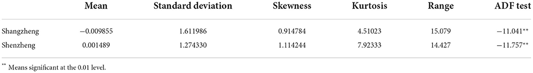
Table 1. Analysis of statistical characteristics of the return rate.

Selection of edge sequence

Since the conditional distribution of financial time series shows the distribution characteristics of wave aggregation, peak, and thick tail, while t-distribution and GED distribution show the distribution characteristics of the thick tail, the GARCH model can well describe the fluctuation law of financial time series. Therefore, GARCH-T or GARCH-GED can be selected to describe the distribution characteristics of the peak, thick tail, and fluctuation aggregation of financial time series. The GARCH-t and GARCH-GED models were used to simulate and analyze the sample data with R software. The simulation result shows that the GARCH (1, 1)-t model can describe the fluctuation rule of each return rate series well. The specific model is as follows:

$\begin{array}{l}{R}_{nt}={\epsilon }_{nt},n=1,2,t=1,2,\cdots ,T\\ {\epsilon }_{nt}=h_{nt}^{\frac{1}{2}}{\xi }_{nt}\\ h_{nt}=W_n+{\alpha }_n{\epsilon }_{n,t-1}^2+{\beta }_n{h}_{n,t-1}\\ ({\xi }_{1t}{,\xi }_{2t})~C(T_{v_1}({\xi }_{1t}),T_{v_2}({\xi }_{2t}))\end{array}$

where T_v1(·) and T_v2(·) express the normalized t-distribution of mean 0, variance 1, the freedom degrees of v₁ and v₂, respectively, namely, ${\sqrt{\frac{v_1}{v_1-2}}\xi }_{1t}~t(v_1){,\sqrt{\frac{v_2}{v_2-2}}\xi }_{2t}~t(v_2)$.

Parameter estimation results of the GARCH model with two edge sequences are shown in Table 2.

TABLE 2

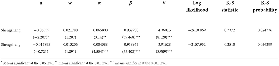
Table 2. Parameter estimation of the GARCH model.

According to the k-s probability value, it can be seen that, by using the estimated conditional marginal distribution, the sequence after the probability integral transformation of the original financial time series can be considered to obey (0, 1) uniform distribution, indicating that the GARCH (1,1)-t model can better simulate the marginal distribution of various financial series.

Selection of copula model

The following is the correlation analysis of the two sequences obtained after the probability integral transformation of the original financial sequence using Clayton, Gumbel, and Frank Archimedes copulas, respectively. The analysis results are as follows:

The Akaike Information Criterion (AIC) is a standard to measure the excellence of statistical model fitting. The smaller the AIC value is, the better the model is. Generally, the model with the smallest AIC is selected. Bayesian Information Criterion (BIC) refers to BIC that is similar to AIC, which is used for model selection. The smaller the value, the better the model is.

According to AIC and BIC criteria in Table 3, the Gumbel copula is selected to describe the interdependence structure between the Shanghai Composite Index and the Shenzhen Composite index. According to the results of the analysis in 2.3,${\lambda }_U(\alpha )=2-2^{\alpha }$, and according to 4-3,α = 0.2857, so λ_U = 0.7810 , λ_L = 0, we can say that there is a strong upper tail dependence between the Shanghai Composite Index and the Shenzhen Composite Index.

TABLE 3

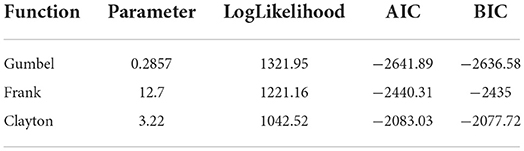
Table 3. Parameter estimation of the copula function.

Selection of asymmetric copula functions

As we know from the previous analysis, the return rates of the Shanghai Composite Index and the Shenzhen Composite Index have a strong upper tail dependence relationship. Here, we select the asymmetric copula function with the distribution characteristics of upper tail dependence for analysis. According to the previous analysis, the asymmetric copula $C^{*}(u,v)=\phi (\frac{1}{2}\sum _{j=1}^2{h}_{j1}({\phi }^{-1}(u))h_{j2}({\phi }^{-1}(v)))$, where $\phi (t)=\frac{{exp(-\alpha {(1-t)}^{\frac{1}{r}})-e}^{-\alpha }}{1-e^{-\alpha }},r\in (1,+\infty ),h_{11}(x)=x^{\frac{3}{2}},h_{21}(x)=2x-x^{\frac{3}{2}},h_{12}(x)=x^2,h_{22}(x)=2x-x^2$, namely, $c^{*}\left(u,v\right)=\phi (\frac{1}{2}({\left({\phi }^{-1}\left(u\right)\right)}^{\frac{3}{2}}{\left({\phi }^{-1}\left(v\right)\right)}^2+\left(2\left({\phi }^{-1}\left(u\right)\right)-{\left({\phi }^{-1}\left(u\right)\right)}^{\frac{3}{2}}\right)(2\left({\phi }^{-1}\left(v\right)\right)-{\left({\phi }^{-1}\left(v\right)\right)}^2)))$, and Gumbel copula are identical in form with the tail-dependence function and the tail-dependence coefficient, and, according to the previous discussion, the upper-tail-dependence coefficient of C^*(u, v) is ${\lambda }_U^{C^{*}}=2-2^{\frac{1}{r}},$ and it is identical in form with Gumbel copula. According to the analysis results in 4.3, the upper- and lower-tail- dependence coefficients of Gumbel copula are, respectively, λ_U = 0.7810 , λ_L = 0, so ${\lambda }_U^{C^{*}}$and ${\lambda }_U^G$can be estimated by empirical tail-dependence functions and empirical tail-dependence coefficients. Therefore, the value ${\lambda }_U^G$ can be used as an estimate of ${\lambda }_U^{C^{*}}$, namely, $2-2^{\frac{1}{r}}=0.78$,so $\widehat{r}=3.5$.

In order to compare the advantages and disadvantages of the asymmetric copula C^*‵, Gumbel copula in describing dependent structures, the square Euclidean distance between asymmetric copula C^*, Gumbel copula, and empirical copula is calculated respectively; the result is as follows: (and $C_i^{*}$ is the asymmetric copula function with α = i. For example, $C_1^{*}$ indicates α = 1).

This is only the case where α = 1, 2... 10. It can be seen from the Euclidean distance in Table 4 that when α = 5, 6, 7, 8, 9, 10, the Euclidean distance between the asymmetric copula C^* and the empirical distribution function is smaller than that between Gumbel and the empirical distribution function, and that, when α = 6 and α = 7, d² minimizes. Both equal 0.0640. The smaller the Euclidean distance is, the higher the fitting degree of the original data is. Therefore, when describing the interdependent structure of financial variables, asymmetric copula shows higher advantages than Archimedean copula. In addition, the asymmetric copula function can also describe the asymmetric interdependent structure between variables, and more truly reflect the interdependent relationship between variables.

TABLE 4

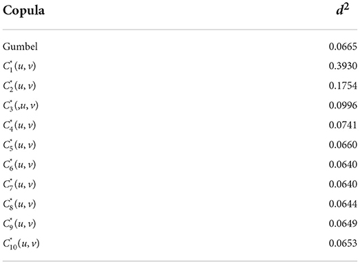
Table 4. d² of C^* (u,v) and Gumbel.

According to the above analysis, the upper-tail-dependence coefficient of the asymmetric copula is only related to parameter r. The larger the value of r is, the larger the value of the tail-dependence coefficient will be. Therefore, we can say that parameter R is a parameter representing the strength of tail dependence. In addition, the Euclidean distance between the copula function and the empirical copula function can be changed by changing the parameter α, and the empirical copula can reflect the overall dependence pattern of the data. Therefore, it can be said that the parameter α is the parameter representing the overall dependence structure. The different parameters of asymmetric copula provide convenience for a more accurate description of the correlation between variables.

Copula correlation coefficient of the asymmetric copula

The biggest advantage of using the asymmetric copula function to describe the interdependent structure of financial variables is that the asymmetric interdependent relationship between financial variables can be explained by the copula correlation coefficient.

According to the discussion in 3.3, at first, the stochastic simulation method is used to generate two independent random sequences (u₁, ⋯, u_n), (v₁, ⋯, v_n),u_i, v_iϵ [0, 1], for some fixed U, and then calculate ${C^{*}}_U(v_i)={\frac{\partial C^{*}(U,V)}{\partial U}|}_{V=v_i}$. Since

$\begin{array}{l}{C}^{*}(U,V)={\phi }^{-1}\left(\frac{1}{2}{(\phi (u))}^{\frac{3}{2}}{(\phi (v))}^2+\frac{1}{2}\left(2\phi (u)-{(\phi (u))}^{\frac{3}{2}}\right)\left(2\phi (v)-{(\phi (v))}^2\right)\right),\text{We can get}\\ {\frac{\partial C^{*}(U,V)}{\partial U}|}_{V=v_i}=\frac{\left(\frac{3}{4}{\phi }^{\frac{1}{2}}(u){\phi }^2(v_i)+\frac{1}{2}\left(2-\frac{3}{2}{\phi }^{\frac{1}{2}}(u)\right)\left(2\left(\phi (v_i)-{\phi }^2(v_i)\right)\right)\right){\left(-ln\left(e^{-\alpha }+u-u{e}^{-\alpha }\right)\right)}^{r-1}exp(-\alpha {(1-s)}^{\frac{1}{r}})}{{(\alpha {(1-s)}^{\frac{1}{r}})}^{r-1}(e^{-\alpha }+u-u{e}^{-\alpha })}\\ r_{V|U}^C(u)\approx {\tilde{r}}_{V|U}^C(u)=1-\frac{1}{n}{\displaystyle \sum _{i=1}^n}{C}_U(v_i)\\ r_{U|V}^C(v)\approx {\tilde{r}}_{U|V}^{C*}(v)=1-\frac{1}{n}{\displaystyle \sum _{i=1}^n}{C}_V(u_i),{\rho }_{2|1}\approx {\tilde{\rho }}_{2|1}=\frac{12}{n}{\displaystyle \sum _{i=1}^n}{\left({\tilde{r}}_{V|U}^{C*}(v_i)\right)}^2-3\end{array}$

where r = 3.5; the result can be obtained by Matlab, ${\tilde{\rho }}_{2|1}=0.3536$. This result shows that 35.36% of the changes in the Shenzhen Composite Index can be explained by the copula regression on the Shanghai Composite Index.

The same method should be used to calculate ${\tilde{\rho }}_{2|1}$. First, for some fixed V, we calculated $C_V^{*}(u_i)={\frac{\partial C^{*}(U,V)}{\partial V}|}_{U=u_i}$,

$\begin{array}{l}{\frac{\partial C^{*}\left(U,V\right)}{\partial V}|}_{U=u_i}=\frac{\left({\phi }^{\frac{3}{2}}\left(u_i\right)\phi \left(v\right)+\left(2\phi \left(u_i\right)-{\phi }^{\frac{3}{2}}\left(u_i\right)\right)\left(1-\phi \left(v_i\right)\right)\right){\left(-ln\left(e^{-\alpha }+v-v{e}^{-\alpha }\right)\right)}^{r-1}exp\left(-\alpha {\left(1-s\right)}^{\frac{1}{r}}\right)}{{\left(\alpha {\left(1-s\right)}^{\frac{1}{r}}\right)}^{r-1}\left(e^{-\alpha }+v-v{e}^{-\alpha }\right)}\\ {\tilde{r}}_{U|V}^{C*}\left(v\right)=1-\frac{1}{n}{\displaystyle \sum _{i=1}^n}{C}_V\left(u_i\right),{\tilde{\rho }}_{1|2}=\frac{12}{n}{\displaystyle \sum _{i=1}^n}{\left({\tilde{r}}_{U|V}^{C^{{}^{*}}}\left(v_i\right)\right)}^2-3,\\ \text{where r}=3.5,\\ {\phi }^{-1}\left(t\right)=\frac{{exp\left(-{\alpha \left(1-t\right)}^{\frac{1}{r}}\right)-e}^{-\alpha }}{1-e^{-\alpha }},\phi \left(t\right)=1-{\left(-\frac{ln\left(e^{-\alpha }+t-t{e}^{-\alpha }\right)}{\alpha }\right)}^r.\end{array}$

Using Matlab to calculate available ${\tilde{\rho }}_{1|2}=0.8450$, the results show that changes in the Shanghai index, 84.5% of the part can be explained by the Shenzhen index on the Shenzhen index Copula regression. The different values of ${\tilde{\rho }}_{1|2}^{\dot{\text{N}}}{\tilde{\rho }}_{2|1}$ illustrate the different relationships between the Shanghai index and the Shenzhen index. It provides conditions for correctly describing the dependence between variables.

Time-varying analysis based on the asymmetric copula function

Because the correlation between variables will change with the change of time, scholars have conducted a lot of research on the dynamic copula model, and some results have been obtained. Deng [34] gave the estimation of Var based on a time-varying copula. Wei and Zhang [35] analyzed the correlation mode and dynamic correlation structure among financial markets, respectively, based on the copula theory and the time series model. Wang et al. [36, 37] analyzed the time-varying correlation model and the variable structure correlation model between financial assets based on Spearman's ρ respectively. However, the symmetric Archimedean copula and elliptic copula were used in most previous analyses. In this paper, we used the asymmetric copula function to analyze the time dependence of variables.

The basic idea of time-varying analysis is to determine the evolution process of the population parameter, according to the dynamic evolution process of the dependent indexes and the correspondence between the dependent indexes and the population parameter. According to the previous analysis, the upper-tail-dependence coefficient ${\lambda }_U(r)=2-2^{\frac{1}{r}}$, and the lower-tail-dependence coefficient λ_L = 0 for the asymmetric copula C^*. Since there is a one-to-one correspondence between the upper-tail-dependence coefficient and the population parameter r, this paper uses the dynamic evolution process of the upper-tail-dependence coefficient to analyze the time variation of asymmetric copula C^*.

Improvement of the dynamic evolution process of the upper-tail-dependence coefficient

Patton [38] was the first to study the time-dependent copula model and proposed that the dynamic evolution process of the parameter ρ of the binary normal copula function could be described by an equation similar to ARMA (1, 10). For tail-dependence coefficients, the commonly used dynamic evolution equation is as follows:

$\begin{array}{ll}{\lambda }_m^U=\Lambda ({\gamma }_U+{\beta }_U{\lambda }_{m-1}^U+{\alpha }_U{W}_m)& (5-1)\end{array}$

$\begin{array}{ll}{\lambda }_m^L=\Lambda ({\gamma }_L+{\beta }_L{\lambda }_{m-1}^L+{\alpha }_L{W}_m)& (5-2)\end{array}$

In the above equation, the function Λ(·) is the logistic transformation function, defined as $\Lambda (x)=\frac{1}{1+e^{-x}}$. The reason why Λ(x) is defined is to ensure that the upper-tail correlation coefficient and the lower-tail correlation coefficient are in the interval of (0, 1) at any time. The right side of the equation includes an autoregressive term and an exogenous variable W_m. There are two common forms of the exogenous variable at present: one is $W_m=\frac{1}{q}\sum _{i=1}^q|u_{m-j}-v_{m-j}|$,; another is ${W^{\prime }}_m=\frac{1}{q}\sum _{i=1}^q{u}_{m-j}{v}_{m-j};q$means the lagging term, where W_m is the mean of the absolute value of the difference between u_i and v_i in the lagging q period, and ${W^{\prime }}_m$ is the mean of the product of dependent random variables u_i and v_i in the lagging q period. If X and Y are positively correlated, U and V are probability integral transformations of X and Y, so U and V are also positively correlated; therefore, the variable will be the main diagonal on the unit square, because |u_t−v_t|, and the point (u_t, v_t) is proportional to the main diagonal of the shortest distance. Therefore, W_mselects the mean of the absolute value of the difference between u_t and v_tin the lag q period as an exogenous variable, and because the tail-dependence coefficient describes the dependence relationship of variables at the extreme value, so ${W^{\prime }}_m$_m selects the mean of the product of two dependent variables in the lag q period as an exogenous variable.

The dynamic evolution process of the tail dependence coefficients above describes the local evolution process of the copula function model to a certain extent. The autoregressive term on the right-hand side of the equation can explain the sustainability of the tail distribution, but in the process of exogenous variables calculation, only using the lag q period data. These data are not necessarily tail data, and the evolution process of the upper tail and the lower tail is uniform in form, so it is not very good to reflect the tail data influence on the tail-dependence coefficient based on this idea. This paper attempts to improve the above evolution equation into the following form:

$\begin{array}{ll}{\lambda }_m^{*U}=\Lambda ({\gamma }_U^{*}+{\beta }_U^{*}{\lambda }_{m-1}^{*U}+{\alpha }_u^{*}{W}_m^{*U})& (5-3)\end{array}$

$\begin{array}{ll}{\lambda }_m^{*L}=\Lambda ({\gamma }_L^{*}+{\beta }_L^{*}{\lambda }_{m-1}^L+{\alpha }_L^{*}{W}_m^{*L})& (5-4)\end{array}$

The function Λ (·) is still the logistic transformation function, defined as $\Lambda (x)=\frac{1}{1+e^{-x}}$

$\begin{array}{l}{W}_m^{*U}=\frac{1}{q}{\displaystyle \sum _{j=1}^q}|u_{m-j}-v_{m-j}|I\left(u_{m-j}>\frac{3}{4},v_{m-j}>\frac{3}{4}\right),\hfill \\ \hfill W_m^{*L}=\frac{1}{q}{\displaystyle \sum _{j=1}^q}|u_{m-j}-v_{m-j}|I\left(u_{m-j}<\frac{1}{4},v_{m-j}<\frac{1}{4}\right)\hfill \end{array}$

Equation 5-3 represents the dynamic evolution equation of the upper-tail-dependence coefficient, and Equation 5-4 represents the dynamic evolution equation of the lower-tail-dependence coefficient.

Exogenous variables can also be taken in the following form:

$\begin{array}{l}{W}_m^{*U}=\frac{1}{q}{\displaystyle \sum _{j=1}^q}{u}_{m-j}{v}_{m-j}I\left(u_{m-j}>\frac{3}{4},v_{m-j}>\frac{3}{4}\right)\\ W_m^{*L}=\frac{1}{q}{\displaystyle \sum _{j=1}^q}{u}_{m-j}{v}_{m-j}I\left(u_{m-j}<\frac{1}{4},v_{m-j}<\frac{1}{4}\right)\end{array}$

In an exogenous variable expression, an indicator function

$\begin{array}{l}I\left(u_{m-j}>\frac{3}{4},v_{m-j}>\frac{3}{4}\right)=\{\begin{array}{cc}1,& \\ & u_{m-j}>\frac{3}{4},v_{m-j}>\frac{3}{4}\\ 0,& \\ & else\end{array}\\ I\left(u_{m-j}<\frac{1}{4},v_{m-j}<\frac{1}{4}\right)=\{\begin{array}{cc}1,& \\ & u_{m-j}<\frac{1}{4},v_{m-j}<\frac{1}{4}\\ 0,& \\ & else\end{array}\end{array}$

By multiplying the indicator function, we can better characterize the dynamic distribution of the variable in the tail.

Here, we still take asymmetric copula C^* as an example to conduct a dynamic analysis of the correlation between financial assets. The analysis steps are as follows:

Step 1. First, the edge distribution of financial time series is modeled.

Step 2. According to the GARCH model selected by the sample data, the original time series is transformed by probability integral, and the marginal distribution is transformed into (0, 1) uniform distribution, and the transformed variables are expressed by (U, V).

Step 3. The statistics of the upper-tail-dependence coefficient should be calculated according to the sample data, and the upper-tail-dependence coefficient sample statistics are as follows:

$\begin{array}{l}{\lambda }^U=\frac{{\displaystyle {\sum }_{i=m}^{950}}I(u_i>\frac{3}{4},v_i>\frac{3}{4})}{{\displaystyle {\sum }_{i=m}^{950}}I(u_i>\frac{3}{4})},m=1,2,\cdots ,900\end{array}$

Step 4. According to the sample data distribution obtained in Step 3, the parameters of the following four dynamic evolution equations are calculated.

$\begin{array}{l}{\lambda }_{1m}^{*U}=\Lambda \left({\gamma }_{1u}^{*}+{\beta }_{1u}^{*}{\lambda }_{1m-1}^{*U}+{\alpha }_{1u}^{*}{W}_{1m}^{*U}\right)\end{array}$

where $W_{1m}^{*U}=\frac{1}{q}\sum _{j=1}^q|u_{m-j}-v_{m-j}|I(u_{m-j}>\frac{3}{4},v_{m-j}>\frac{3}{4})$;

$\begin{array}{l}{\lambda }_{2m}^{*U}=\Lambda \left({\gamma }_{2u}^{*}+{\beta }_{2u}^{*}{\lambda }_{2m-1}^{*U}+{\alpha }_{2u}^{*}{W}_{2m}^{*U}\right)\end{array}$

where $W_{2m}^{*U}=\frac{1}{q}\sum _{j=1}^q{u}_{m-j}{v}_{m-j}I(u_{m-j}>\frac{3}{4},v_{m-j}>\frac{3}{4})$;

$\begin{array}{l}{\lambda }_{1m}^U=\Lambda \left({\gamma }_{1U}+{\beta }_{1U}{\lambda }_{1m-1}^U+{\alpha }_{1U}{W}_{1m}^U\right)\end{array}$

where $W_{1m}^U=\frac{1}{q_0}\sum _{j=1}^{q_0}|u_{m-j}-v_{m-j}|$;

$\begin{array}{l}{\lambda }_{2m}^U=\Lambda \left({\gamma }_{2U}+{\beta }_{2U}{\lambda }_{2m-1}^U+{\alpha }_{2U}{W}_{2m}^U\right)\\ \hfill \text{where }{W}_{2m}^U=\frac{1}{q_0}{\displaystyle \sum _{j=1}^{q_0}}(u_{m-j}{v}_{m-j})\end{array}$

Improved dynamic evolution equation, the exogenous variables of considering only the tail $u_i>\frac{3}{4},v_i>\frac{3}{4}$ ; thus, the amount of data involved in calculating reduces; in order to improve the fitting accuracy, the lag period q of the improved dynamic evolution equation of the lag period is chosen to 20, and the lag periods of the original dynamic evolution equation, in general, are chosen to 10.

Step 5. ${\lambda }_m^U$ is estimated according to the obtained dynamic evolution equations, and the square root of the mean square error is calculated for the estimated values and sample values of the four evolution equations.

RMSE $={(\frac{1}{N}\sum {(\widehat{\lambda }-\lambda )}^2)}^{\frac{1}{2}}$. The advantages and disadvantages of four kinds of dynamic evolution equations are judged. In this paper, the dynamic evolution equation, which minimizes the square root of the mean square error, is selected for further analysis.

Step 6. Finally, by using the selected dynamic evolution equation, according to the one-to-one correspondence between the upper-tail-dependence coefficient and the population parameter, the estimated value of the population parameter is obtained so as to dynamically analyze the dependence relationship between the Shanghai Composite Index return rate and the Shenzhen Composite Index return rate.

Empirical analysis

The Shanghai Composite Index and the Shenzhen Component Index are still selected as research objects (represented by X₁ and X₂, respectively). Stock The stock price is defined as the daily closing price P_t,. The time span of sample selection is from 31 July 2015 to 27 September 2021, with a total of 1,500 valid data. The return rate of financial asset X_i on the t trading day R_jt = 100 (ln P_nt − lnP_nt−1). According to the previous analysis, the GARCH (1,1) -t model can be used to describe the probability distribution of each return rate series. The GARCH (1,1) -t model can be used to describe the probability distribution of each return rate series. The sequence (u_i, v_i) is obtained by the probability integral transformation of the original sequence X₁ and X₂, i = 1, 2, ⋯, 1, 500.

1. The sample sequence (u_i, v_i) should e selected, i = 1, 2, ⋯, 900, and the statistical value of the upper- tail- dependence coefficient ${\lambda }_m^U$ should be calculated by using the statistics defined in Step 3, as shown below:

$\begin{array}{l}{\lambda }^U=\frac{{\displaystyle {\sum }_{i=m}^{900}}I\left(u_i>\frac{3}{4},v_i>\frac{3}{4}\right)}{{\displaystyle {\sum }_{i=m}^{900}}I\left(u_i>\frac{3}{4}\right)},m=1,2,\cdots ,850\end{array}$

where the numerator and the denominator are sliding window data. In the above equation, the maximum value of m is 850. In the definition of 5.1 λ^U, the maximum value of m is 900. The reason for this choice in the paper is that it is found in the data analysis process that, if the maximum value of m is selected as 850, the advantages of describing the dynamic dependence relationship between variables are more obvious according to the improved dynamic evolution equation. In order to fully demonstrate the advantages of the improved dynamic evolution equation in theory and practice, the maximum value of m is selected as 850 in the empirical analysis.

According to Figure 1, λ^Uincreases with the increase of m, indicating that, for the sample sequence (u_i, v_i), i = 1, 2, ⋯, 900, the larger the m is, the further the position of the sliding window is, the further the data involved in the calculation are, and the smaller the amount of data is. At this point, when $\left(u_i>\frac{3}{4}\right),i=m,m+1,\cdots ,900$, the number of $\left(v_i>\frac{3}{4}\right)$also increases. As shown in Figure 1, the statistical value of λ^U reaches the maximum when the sliding window is located at m = 700, indicating that, under the conditions of $\left(u_i>\frac{3}{4}\right),i=700,701,\cdots ,900$. The number of data that simultaneously satisfies $\left(v_i>\frac{3}{4}\right)$ is largest. Through calculation, it is found that the statistical values of ${\lambda }_m^U$ swing around 0.8. In the previous static analysis of the Shanghai Composite Index and the Shenzhen Component Index, the estimated value of the upper-tail-dependence coefficient is 0.7809863, close to 0.8. Therefore, the estimated value of the upper-tail-dependence coefficient in the static analysis is basically consistent with the results of the dynamic analysis.

FIGURE 1

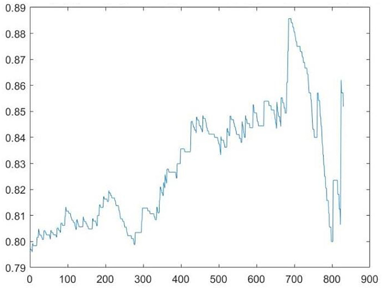
Figure 1. A dynamic diagram of upper- tail-dependence coefficients statistics.

2. The estimated values of the four model parameters are obtained using the statistics of ${\lambda }_m^U$, as shown in the table below:

3. The four dynamic evolution equations were used to estimate the upper-tail-dependence coefficients, and the square root of the mean square error (RMSE) of the estimated value and the sample value were calculated. RMSEs were expressed as $d_1^{*},d_2^{*},d_1,d_2$, respectively. The calculated results are shown in the following table:

It can be seen from the table that the RMSEs of the two improved dynamic evolution equations are both smaller than that of the original dynamic evolution equation, indicating that the improved dynamic evolution equation can more accurately depict the dynamic evolution process of the upper-tail-dependence coefficient compared with the original dynamic evolution equation.

In fact, according to the values of (u_i, v_i), it can be seen that some pairs of (u_i, v_i) do not belong to the upper tail data. It is obviously not appropriate to calculate the upper-tail-dependence coefficients directly based on all values of (u_i, v_i). It is theoretically more feasible to select the upper-tail data by multiplying the function of expression to calculate the upper-tail-dependence coefficients. According to Table 9, $d_1^{*}$ is 3 × 10⁻⁵smaller than d₁, and $d_2^{*}$ is 2 × 10⁻⁵ smaller than d₂,; the difference is relatively small. The reasons for the small difference are as follows: (1) By multiplying the exogenous variable by an explicit function, the value of the exogenous variable will be smaller than that of the original exogenous variable; however, according to Tables 5–8 it can be seen that the absolute values of the coefficient ${\alpha }_{1u}^{*}$ and ${\alpha }_{2u}^{*}$ of the exogenous variable in the improved dynamic evolution equation increase. Therefore, after multiplying the improved exogenous variable and its coefficient, the larger and smaller parts will cancel each other. There is not much difference between $d_i^{*}$ and d_i(i = 1, 2) on the surface. (2) The difference between $d_i^{*}$ and d_i(i = 1, 2) becomes smaller due to a large amount of data. Although the difference between $d_i^{*}$ and d_i is not large, theoretically, the improved dynamic evolution equation is more reasonable, and the value of $d_i^{*}$ is smaller, and the dynamic evolution process of the tail-dependence coefficient can be described more accurately.

TABLE 5

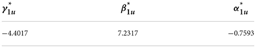
Table 5. Parameters estimates of the time-varying model for the upper-tail-dependence coefficients ${\lambda }_{1m}^{*U}$.

TABLE 6

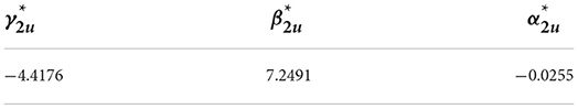
Table 6. Parameters estimates of the time-varying model for the upper-tail-dependence coefficients ${\lambda }_{2m}^{*U}$.

TABLE 7

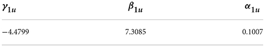
Table 7. Parameters estimates of the time-varying model for the upper-tail-dependence coefficients ${\lambda }_{1m}^U$.

TABLE 8

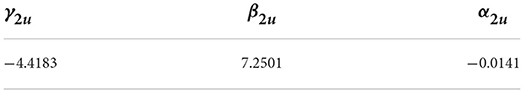
Table 8. Parameters estimates of the time-varying model for the upper-tail-dependence coefficients ${\lambda }_{2m}^U$.

In addition, among the two improved dynamic evolution equations, the RMSE corresponding to the exogenous variable $W_{1m}^{*U}$ is smaller than that corresponding to the exogenous variable $W_{2m}^{*U}$, indicating that it is more appropriate to choose the exogenous variable $W_{1m}^{*U}$. However, according to Table 9, the difference between $d_1^{*}$ and $d_2^{*}$ is very small. It shows that there is no significant difference between the two types of exogenous variables in the dynamic analysis of the Shanghai Stock index and the Shenzhen Stock index.

TABLE 9

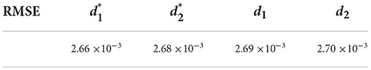
Table 9. RMSE values of estimated values and sample values.

4. The selected dynamic evolution equation should be used to calculate the estimated value of λ^uand draw the dynamic evolution diagram of the estimated value and the sample value, as shown in the figure below:

As can be seen from Figure 2, the estimated value and the sample value calculated by using the dynamic evolution equation are highly consistent in both trends and fluctuation, which fully demonstrates that dynamic evolution Equation 5-3 can accurately depict the dynamic evolution process of the upper-tail-dependence coefficient.

FIGURE 2

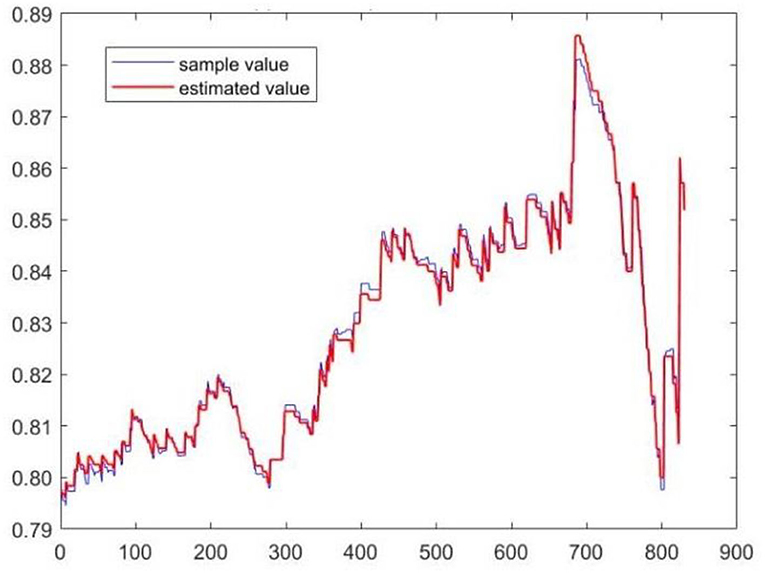
Figure 2. A dynamic diagram of statistics and estimates of upper-tail-dependence coefficients.

5. According to the correspondence between the upper-tail-dependence coefficient λ^uand the population parameter r, ${\lambda }^u(r)=2-2^{\frac{1}{r}}$, the dynamic estimate of the population parameter r is obtained, as shown below Figure 3.

FIGURE 3

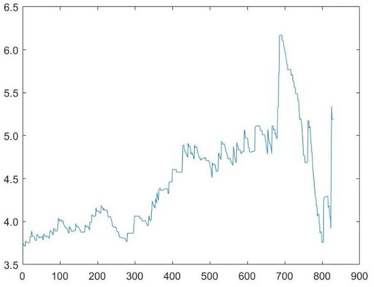
Figure 3. A dynamic diagram of the population parameters estimation.

Conclusion

In the correlation analysis of financial assets, symmetric Archimedes copula and elliptic copula functions are mostly used for analysis, and the dependence indicators between variables are also mostly symmetric, which does not conform to the relationship characteristics between financial assets. Based on this, this paper tries to conduct static and dynamic analyses on the correlation of financial assets based on the asymmetric copula. In the static analysis, through the comparative analysis of the asymmetric copula function and the Gumbel copula function, it is found that the asymmetric copula function has more advantages in depicting tail dependence between financial assets. Furthermore, this paper also introduced the concept of the asymmetric copulas correlation coefficient. For the asymmetric copula function, copula correlation coefficients ρ_1|2 and ρ_2|1 are not equal; and asymmetric dependence between variables can be explained by the copula correlation coefficient, which also shows the great advantages of the asymmetric copula. In the dynamic analysis, the traditional dynamic evolution equation is improved through the empirical analysis, which shows that the improved dynamic evolution equation more accurately portrays the tail-dependence dynamic evolution process, since there is a one-to-one correspondence between the upper-tail-dependence coefficient λ^u and the population parameter; according to the dynamic evolution equations of λ^u, the population parameter can be estimated. Thus, the interdependence between financial assets is analyzed asymmetrically and dynamically.

Through empirical analysis, it can be seen that asymmetric copula has more advantages in describing the dependence relationship between financial assets compared with the commonly used Archimedean copula. The asymmetric copula is more suitable for the dependence structure between financial variables. However, for asymmetric copula function, it is difficult to estimate the parameters due to the complex form. In this paper, the Archimedean copula is first used to analyze the correlation between the Shanghai Stock index and the Shenzhen Stock index, and the empirical dependence coefficient of the tail is used to estimate the parameters of the asymmetric copula. Therefore, the asymmetric analysis is developed on the basis of the symmetric analysis. Although the asymmetric copula function is superior to the symmetric copula in application, it is difficult to make further progress in asymmetric copula analysis without some conclusions obtained from symmetric copula analysis. The analysis of asymmetric dependence between variables is one of the advantages of the asymmetric copula, but the calculation of the asymmetric dependence coefficient defined on the basis of the asymmetric copula is more difficult. In this paper, the method of Monte Carlo simulation is used to estimate the dependence coefficient. Therefore, how to estimate the parameters and calculate the dependence coefficient of asymmetric copula more easily is the problem to be studied in the following paper.

Data availability statement

The original contributions presented in the study are included in the article/Supplementary material, further inquiries can be directed to the corresponding author.

Author contributions

All authors listed have made a substantial, direct, and intellectual contribution to the work and approved it for publication.

Conflict of interest

The authors declare that the research was conducted in the absence of any commercial or financial relationships that could be construed as a potential conflict of interest.

Publisher's note

All claims expressed in this article are solely those of the authors and do not necessarily represent those of their affiliated organizations, or those of the publisher, the editors and the reviewers. Any product that may be evaluated in this article, or claim that may be made by its manufacturer, is not guaranteed or endorsed by the publisher.

Supplementary material

The Supplementary Material for this article can be found online at: https://www.frontiersin.org/articles/10.3389/fams.2022.1005956/full#supplementary-material

References

1. Romano C. Calibrating and Simulating Copula Functions: An Application to the Italian Stock Market. Working paper, CIDEM. (2002).

Google Scholar

2. Rosenberg JV, Schuermann T. A general approach to integrated risk management with skewed, fat-tailed risks. J Financ Econ. (2006) 79:569–614. doi: 10.1016/j.jfineco.2005.03.001

CrossRef Full Text | Google Scholar

3. Patton AJ. Modelling asymmetric exchange rate dependence. Int Econ Rev. (2006) 47:527–56. doi: 10.1111/j.1468-2354.2006.00387.x

CrossRef Full Text | Google Scholar

4. Patton AJ. Application of copula theory in financial econometrics. Doctor Thesis, San Diego: Department of Economics, University of California, San Diego. (2002).

Google Scholar

5. Palaro HP, Hotta LK. Using conditional copula to estimate value at risk. J Data Sci. (2006) 4:93–115. doi: 10.6339/JDS.2006.04(1).226

CrossRef Full Text | Google Scholar

6. Nikolai K, Anjos U, Mendes BVM. Copulas: a review and recent developments. Stochastic Models. (2006) (4):617–60. doi: 10.1080/15326340600878206

PubMed Abstract | CrossRef Full Text | Google Scholar

7. Zhang YT. Copula technology and financial risk analysis. Stat Res. (2002) 4:48–51. doi: 10.19343/j.cnki.11-1302/c.2002.04.011

CrossRef Full Text

8. Zhang MH. Research on the Copula measurement method of Value at risk of multiple financial assets. J Quant Tech Econ. (2004) 21:67–70. doi: 10.13653/j.cnki.jqte.2004.04.011

CrossRef Full Text

9. Wu ZX, Chen M, Ye WY, Miao BQ. Analysis of foreign exchange portfolio risk based on Copula. Chin J Manage Sci. (2004) 12:1–5. doi: 10.16381/j.cnki.issn:1003-207x.2004.04.001

CrossRef Full Text

10. Wang PJ, Wen GH, Huang TW, Yu WW, Lü YZ. Asymptotical neuro-adaptive consensus of multi-agent systems with a high dimensional leader and directed switching topology. In: IEEE Transactions on Neural Networks and Learning Systems. (2022). doi: 10.1109/TNNLS.2022.3156279

PubMed Abstract | CrossRef Full Text | Google Scholar

11. Wu ZX, Chen M, Ye WY, Miao BQ. Portfolio risk analysis based on Copula GARCH. Syst Eng Theor Pract. (2006) 26:45–52. doi: 10.3321/j.issn:1000-6788.2006.03.007

CrossRef Full Text

12. Wei YH, Zhang SY. Correlation analysis of financial market: copula GARCH model and its application. Syst Eng. (2004) 22:7–12. doi: 10.3969/j.issn:1001-4098.2004.04.002

CrossRef Full Text

13. Wei YH, Zhang SY. Research on dynamic correlation structure of financial market. J Syst Eng. (2006) 21:313–7. doi: 10.3969/j.issn:1001-45781.2006.03.015

CrossRef Full Text

14. Zhang JQ, Li X. Integrated risk measurement of asset portfolio and its application: research on VaR based on optimal fitting copula function. Syst Eng Theor Pract. (2008) 6:23–6. doi: 10.3321/j.issn:1000-6788.2008.06.002

CrossRef Full Text

15. Wang PJ, Wen GH, Huang TW Yu WW, Ren Y. Observer-based consensus protocol for directed switching networks with a leader of nonzero inputs. IEEE Trans Cybern. (2022) 52:630–40. doi: 10.1109/TCYB.2020.2981518

PubMed Abstract | CrossRef Full Text | Google Scholar

16. Li M, Liu XB, He H, Yao, P. Measurement of portfolio VaR based on clayton Copula-GARCH model. Pract Understand Mathem. (2013) 6:51–4. doi: 10.3969/j.issn:1000-0984.2013.06.017

CrossRef Full Text

17. Du ZP, Zhang XF. Comparative study of two kinds of mixed rattan copula model: based on VaR of foreign exchange asset portfolio. Technl Econs Manag Res. (2014) 1:27–31.

18. Ren XL, Zhang SY. Analysis of investment risk based on kernel estimation and multiple archimedes copula. Manage Sci. (2007) 20:92–97. doi: 10.3969/j.issn:1672-0334.2007.05.012

CrossRef Full Text

19. Clayton DG. A model for association in bivariate life tables and its application in epidemiological studies of familial tendency in chronic disease incidence. Biometrika. (1978) 65(1):141–151. doi: 10.1093/biomet/65.1.141

CrossRef Full Text | Google Scholar

20. Frank MJ. On the simultaneous associativity of F(x,y) and x+y-F(x,y). Aequ Math. (1979) 19:194–226. doi: 10.1007/BF02189866

CrossRef Full Text | Google Scholar

21. Gumbel EJ. Distributions des valeurs extrêmes en plusiers dimensions. Publ. Inst. Statist. Univ. Paris. (1960) 9:171–173.

Google Scholar

22. Joe H. Multivariate Models and Dependence Concepts. London: Chapman & Hall. (1997). doi: 10.1201/9780367803896

CrossRef Full Text

23. Alfonse AE, Brigo D. New families of Copulas based on periodic function. Comn Statist Theory Methods. (2005) 34:1437–47. doi: 10.1081/STA-200063351

CrossRef Full Text | Google Scholar

24. Khoudraji A. Contributions à l' étude des Copulas et à la modélisation des valeurs extrêmes bivaviées. Ph.D Thesis, Canada: Université Lavab Quebec. (1995).

Google Scholar

25. Liebscher E. Construction of asymmetric multivariate Copulas. J Multivar Anal. (2008) 99:2234–50. doi: 10.1016/j.jmva.2008.02.025

CrossRef Full Text | Google Scholar

26. Nelsen RB. An Introduction to Copulas. New York: Springer. (2006).

Google Scholar

27. Sungur EA. Some observations on Copula regression functions. Stat Theory Methods. (2005) 34:1967–78. doi: 10.1080/03610920500201244

CrossRef Full Text | Google Scholar

28. Dabrowska D. Regression-based orderings and measures of stochastic dependence. Math Oper Forsch Stat Ser Stat. (1981) 12:317–25. doi: 10.1080/02331888108801592

CrossRef Full Text | Google Scholar

29. Dette H, Siburg KF, Stoimenov PA, A Copula-based non-parametric measure of regression dependence. Scand J Stat. (2013) 40:21–41. doi: 10.1111/j.1467-9469.2011.00767.x

CrossRef Full Text | Google Scholar

30. Shih JH, Emura T. On the Copula Correlation ratio and its generalization. J Multivar Anal. (2021) 182:104708. doi: 10.1016/j.jmva.2020.104708

CrossRef Full Text | Google Scholar

31. Darsow WF, Nguyen B, Olsen ET. Copulas and Markov processes. Illinois J Math. (1992) 36:600–42. doi: 10.1215/ijm/1255987328

CrossRef Full Text | Google Scholar

32. Kim DY, Kim JM. Analysis of directional dependence using asymmetric Copula-based regression models. J Stat Comput Simul. (2014) 84:1990–2010. doi: 10.1080/00949655.2013.779696

CrossRef Full Text | Google Scholar

33. Sungur EA. A note on directional dependence in regression setting. Comm Statist Theory Methods. (2005) 34:1957–65. doi: 10.1080/03610920500201228

CrossRef Full Text | Google Scholar

34. Deng GM. The VaR Estimating on Time-varying Copula. Syst Eng. (2007) 25:28–33. doi: 10.3969/j.issn:1001-4098.2007.08.005

CrossRef Full Text

35. Wei YH, Zhang SY. Copula Theory and its Application in Financial Analysis. Beijing: Qing dynasty Hua University Press. (2008).

36. Wang Q, Wang L, Cheng SJ. Analysis of the Interdependence of Shanghai and Shenzhen stock markets based on time-varying Copula Model. Statist Decis. (2010) 19:139–41. doi: 10.13546/j.cnki.tjyjc.2010.19.002

CrossRef Full Text

37. Wang Q, Wang L, He P. Spearman based time-varying Copula module Simulation and Application of type 2. Mathem Statist Manage. (2011) 1:76–84. doi: 10.13860/j.cnki.sltj.2011.01.007

CrossRef Full Text

38. Patton AJ. Modeling time-varying exchange rate dependence using conditional copula. Working Paper of Department of Economics, University of California, San Diego. (2001). doi: 10.2139/ssrn.275591

CrossRef Full Text | Google Scholar