Bias reduction in the logistic model parameters with the LogF(1,1) penalty under MAR assumption

1. Introduction

Statistical model parameter estimation is a major process requiring improved methods because its a basis for informed decisions, which in most cases rely on data. Complete and incomplete data alike may suffer from biases that may arise from the methods of estimations. Careful scrutiny and efforts have been made to generate some remarkable reduction in bias of estimated model parameters [1, 2]. Penalizing the log-likelihood with a suitable prior distribution is known to reduce bias in model parameters. Bias reduction under conditions of missing data in the estimated parameters has received little research attention in the past, drawing a few studies, also with different focus in scope and coverage. Furthermore, recent studies that have attempted to derive bias reduction methods, under missing data conditions have tried only for the case of missingness in the outcome variable [3, 4].

The estimation process of the logistic regression requires that datasets are complete, besides observing a set of other model assumptions. However, in reality and for various reasons, it is difficult for some vital studies to generate complete datasets. Commonly, missing data are handled by using list-wise deletion method which drops any data item containing missing values. However, dropping cases reduces the sample size [5] and this plays negatively on the predictability and application of the fitted model. For the logistic model, it is well-known that with a small sample size the maximum likelihood estimates will be biased. In 1993, Firth proposed a method which resulted in the second order [O(n⁻²)] bias reduction of the estimates [6]. Moreover, data separation, especially for the case of a binary outcome is yet another problem since the estimates are obtained using an iterative process such as the Newton-Raphson method. In 2006, Heinz found that Firth's method could also solve the separation problem to a certain level of efficiency [7–9]. Moreover in 2016, Carlisle noted that the separation problem could also be handled by using a well-tested prior distribution [10].

A recent study with a focus on bias reduction was by Little and Rubin [11]. Previously in 1990, Ibrahim [12] proposed an estimation method for incomplete covariates for a generalized linear model (GLM) by using the expectation-maximization (EM) algorithm. Followed by Ibrahim and Lipsitz [13], who applied the EM algorithm to estimate the logistic regression parameters when some of the responses were missing. Consequently, Das et al. [14] proposed a bias reduction for the logistic model under MAR assumption following the Firth approach by applying Ibrahim's EM method which achieved a second order bias reduction. In addition, Maity et al. adopted the Lipsitz and Ibrahim EM algorithm, and they came up with another bias reduction method for the logistic model under the incomplete response problem and the MNAR mechanisms, which attempted to reduce the bias as well as the separation problem [15, 16]. Overall, however, chronology shows sparsity of studies that focus specifically on achieving more accurate parameter estimates under the incomplete covariates' data since most of the attempts have focussed on the missing data in the outcome variable.

Our current study is guided by the success derived from other related complete data studies from which the choice of a penalty distribution is drawn. For the complete case, it was demonstrated that the LogF(m,m) family of distributions could provide a reliable penalty of the logit model [17]. Incidentally, no study has tested this hypothesis for the bias reduction under the missing at random (MAR) data problem.

2. Motivating example

In an exploratory analysis, we analyzed data from a survey meant to determine intensive care unit (ICU) admission risk factors in a study conducted at the Royal Hospital in the Sultanate of Oman [18]. To motivate the need of bias reduction method for estimated parameters, we considered only the significant covariates which are the independent predictors of the ICU admission for the COVID-19 patients. The selected covariates were; having conjuctivitis, being unconscious and having a neurological problem, whereas the response variable was whether the patient was admitted to the ICU. The proportion of missing data for each explanatory variable are; conjuctivitis (34%), unconscious (2%), and neurological (4%). We explored by fitting a logistic model for ICU admission. The results are summarized in Figure 1.

FIGURE 1

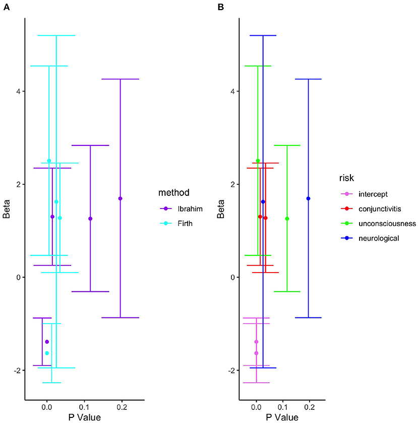
Figure 1. Bias reduction under the Ibrahim and firth methods. (A) Beta vs. P by method. (B) Beta vs. P by risk.

It was observed that, for example being unconscious could be interpreted as not significant under the Ibrahim's method yet it is significant under the Firth's method for bias reduction. Further, the predictor, neurological, under both the Ibrahim's and Firth's methods could not be considered significant with noticeably higher standard errors under the Firth than Ibrahim's method. Therefore, what method is best suited for drawing reliable statistical inference to such a problem? Why do the two methods, that are thought to reduce bias in the model parameters perform differently on the same data? Could penalization improve the performance in parameter estimation? To address these questions, we propose and validate a novel bias reduction method, as demonstrated in the preceeding sections.

Consequently, in this current study, we propose a novel method to reduce bias in the model parameters through penalizing the log-likelihood function, based on the EM method of weight for estimation of incomplete binary categorical covariates. Moreover, we also derive a closed form for the bias for estimated parameter by applying the Cox and Snell's equation, which is based on the Taylor's series [19]. The information matrix was developed using the Louis' method [20]. The main contribution of this study is the novel method, which is quite competitive in parameter estimation under the MAR data mechanism. The method is validated to respond to questions such as; can penalization result in bias reduction of the estimated parameters when the binary response is complete, but some categorical covariates are stochastically missing? What is the better penalty function to apply? How competitive is the novel approach compared to the available methods? Using the proposed method, and as an application, what are the determinants of ICU admission due to COVID-19?

The rest of the paper is organized as follows; in Section 3, we present theoretical methods as the building blocks for the study, Section 4 provides some results focussing on model validation through simulation as well as application using the real life data, and in Section 5, we present a discussion and draw conclusions for the study.

3. Methods

3.1. Definitions and notation

Three important missingness mechanisms have been defined [21] and these are mainly being attributed to the data rather than the distribution of missingness [22, 23]. Among them is the missing at random (MAR) mechanism, which is the main focus of this study, briefly defined here:

Definition 1. Let y = (y₁, y₂, ⋯ , y_n) be a realization of the random sample from an infinite population with density f(y; θ₀). Let δ_i be an indicator function defined by

${\delta }_i=\{\begin{array}{ll}1& \text{if }{y}_{i}isobserved\\ 0& \text{if }{y}_{i}otherwise\end{array}$

Let's assume P(δ_i = 1|y_i) = π(y_i, ϕ) for some parameter ϕ and that π(.) is a known function. Thus, if instead of observing (δ_i, y_i) directly, we do observe (δ_i, y_{i, obs}), where the y_obs = y_obs(y, δ) and y_{i, obs} is defined as

$y_{i,obs}=\{\begin{array}{cc}{y}_i& \text{if }{\delta }_i=1\\ *& \text{if }{\delta }_i=0\end{array}$

The missing data mechanism is MAR if

$p(\delta |y)=p(\delta |y_{obs})$

for all y₁ and y₂ satisfying y_obs(y₁, δ) = y_obs(y₂, δ).

This implies that under the MAR mechanism, the response mechanism p(δ|y) depends on y only through y_obs. If we let y = (y_obs, y_mis), then by the Bayes' theorem $p(y_{mis}|y_{obs,\delta })=\frac{p(\delta |y_{mis}{y}_{obs})}{p(\delta |y_{obs})}=p(y_{mis}|y_{obs})$. Consequently, the two other mechanisms can be defined as missing completely at random (MCAR), which occur when p(δ|y) $\cancel{\propto }$ y, whereas not missing at random (NMAR) occurs when p(δ|y) ≠ p(δ|y_obs). Our study focusses on the MAR data mechanism. However, though the MNAR may have been more plausible, it is known to rely mainly on unstable model assumptions. Moreover, every MCAR data are by default also MAR, and the MNAR data are not ignorable.Let θ be the parameter vector for data model, and Ψ is the parameter vector for missingness mechanisms, so the full-likelihood can be written as:

$\begin{array}{l}L(\theta ,\text{Ψ},y_{obs},\delta )=\int f_Y(y_{obs},y_{mis}|\theta )f_{(M|y)}(\delta |y_{(obs)},y_{(mis)},\text{Ψ})\\ d{y}_{(mis)}\end{array}$

Theorem 1. The missingness mechanisms is ignorable for the direct likelihood inference(m, y_obs) if the following two condition hold:

• Parameter distinctness: two parameters θ and Ψ are distinct, in the sense that the joint parameter space (θ, Ψ) say, Ω_{θ, Ψ}, is the product of the parameter space Ω_θ of θ and the parameter space Ω_Ψ of Ψ that is, Ω_{θ, Ψ}= Ω_θ × Ω_Ψ.

• Factorization of the full likelihood with (y_obs, δ) factors as:

$\begin{array}{l}{L}_{full}(\theta ,\text{Ψ}|y_{obs,\delta })=L_{ignore(\theta |y_{obs})}\times L_{rest}(\text{Ψ}|y_{obs},\delta )\forall \\ \theta ,\text{Ψ}\in {\Omega }_{\theta ,\text{Ψ}}& (1)\end{array}$

Corollary 1.1. If the missing data are MAR at (δ, y_obs) with θ and Ψ distinct, then we can say that the missingness mechanisms is ignorable for the likelihood inference.

Penalized regression methods have been used to assess the best fit for the complete-case [24].

Definition 2. Assume a regression model, y = Xβ and a loss function of the parameter estimate θ, therefore Q(θ), the resulting loss function will be the summation of the squared error loss and a penalty term. The penalized regression is defined as

$Q(\theta )=L(\theta |\text{X})+\omega p(\theta )={(y-\text{X}\beta )}^{{}^{\prime }}(y-\text{X}\beta )+\omega p(\beta )$

where, $Y\in {\Re }^n,{\mathbf{\text{X}}}_{nxp},\beta \in {\Re }^p$, and ω is a lagrange coefficient. The ωp(β) penalty term may also be referred to as a regularization term.

3.2. The EM by the method of weights

Let y₁, y₂, ..., y_n be independent Bernoulli random variables and x, the matrix of regressors of order n × d, where d is the number of regressors. For completely observed data, π_i = (P(y_i = 1|x, β) where $\beta ={({\beta }_0,{\beta }_1,{\beta }_2,...,{\beta }_p)}^{\prime }$ are the unknown parameters [12]. The logistic model relates π_i to x as $log\frac{{\pi }_i}{(1-{\pi }_i)}={\mathbf{\text{x}}}^{\prime }\beta$, and the likelihood written as $L={\Pi }_{i=1}^{n}P(y_i|\mathbf{\text{x}},\beta )$.

Let P(x|α) be the marginal density of x where α is the indexing nuisance parameter. Therefore, for θ = (β, α) the complete log likelihood is:

$\begin{array}{ll}\ell (\theta ,\text{x},y)={\displaystyle \sum _i}\ell (\theta ,x_i,y_i)={\displaystyle \sum _i}{\ell }_{y_i|x_i}(\beta )+{\ell }_{x_i}(\alpha )& (2)\end{array}$

Where, ℓ_yi|xi(β) = log(P(y_i|x_i, β)) and ℓ_xi(α) = log(P(x_i|α)). Suppose further that x_i = (x_{obs, i}, x_{mis, i}), then the E-step at the (t + 1)th iteration of the log-likelihood using EM algorithm becomes:

$\begin{array}{ll}\begin{array}{c}Q(\theta |{\theta }^{(t)})={\displaystyle \sum _{i=1}^n}{\displaystyle \sum _{x_{mis},i(j)}}{w}_{ij}^{(t)}\ell (\theta ;x_i,y_i)\\ ={\displaystyle \sum _{i=1}^n}{\displaystyle \sum _{x_{mis},i(j)}}{w}_{ij}^{(t)}log\left[P(y_i|x_i,\beta )\right]\\ +{\displaystyle \sum _{i=1}^n}{\displaystyle \sum _{x_{mis},i(j)}}{w}_{ij}^{(t)}log\left[P(x_i|\alpha )\right]\\ =Q^{(1)}(\beta |{\theta }^{(t)})+Q^{(2)}(\alpha |{\theta }^{(t)})\end{array}& (3)\end{array}$

Where, θ^(t) is the estimate obtained at the tth iteration in the EM. Note that in the equation above, the inner sum is taken over all possible distinct missing pattern indexing j for each subject i. By using the Bayes' theorem, the weight w_(ij) can be written as

$\begin{array}{l}{w}_{ij}^{(t)}=P(x_{mis},i(j)|x_{obs,i},y_i,{\theta }^{(t)})\\ =\frac{P(y_i|x_{mis},i(j),x_{obs,i},{\theta }^{(t)})P(x_{mis,i}(j),x_{obs,i}|{\theta }^{(t)})}{{\displaystyle {\sum }_{xmis,i(j)}}P(y_i|x_i,{\theta }^{(t)})P(x_i|{\theta }^{(t)})}& (4)\end{array}$

The E-step is a sum of two functions with different parameters, while the M-step involves two separate maximizations. Maximizing Q⁽¹⁾ gives the score function: $U(\beta )=\sum _{i=1}^n\sum _{xmis,i,(j)}{w}_{ij}{x}_i(y_i-{\pi }_i)$ and the information matrix I(β) = x′π(1 − π)wx, where the maximization is done iteratively using the relation β^(t+1) = β^(t) + I(^β(t))−1U(β^(t)).

Based on this approach, we proposed a novel method for bias reduction for the logistic model under MAR assumption as in the proceeding sections.

Theorem 2 (monotonicity property). Every EM algorithm increases ℓ(θ|y_obs) at each iteration that is:

$\ell ({\theta }^{(t+1)}|y_{obs})\ge \ell ({\theta }^{(t)}|y_{obs})$

This theorem implies that as the EM algorithm iterates, the (t + 1)th guess (θ)^(t+1) will never be less than tth guess θ^t. This satisfies the monotonicity property of the EM algorithm. That is ℓ(θ|y_obs) is non-decreasing on each iteration of the EM algorithm, and is strictly increasing on any iteration, such that the Q-function increases, that is $Q({\theta }^{(t+1)}|{\theta }^{(t)},y_{obs})>Q({\theta }^{(t)}|{\theta }^{(t)},y_{obs})$

Proof. Let Y be the complete data which can be factored as:

$\begin{array}{ll}f(Y|\theta )=f(y_{obs},y_{mis}|\theta )=f(y_{obs}|\theta )f(y_{mis}|y_{obs},\theta )& (5)\end{array}$

where f(Y_obs|θ) is the density of the Y_obs and f(Y_mis|Y_obs, θ) is the density of the missing data given the observed data.

Then, the log-likelihood decomposition corresponding to (1) is:

$\begin{array}{ll}\ell (\theta |Y)=\ell (\theta |Y_{obs},Y_{mis})=\ell (\theta |Y_{obs})+lnf(Y_{mis}|Y_{obs},\theta )& (6)\end{array}$

We seek to estimate θ by maximizing the incomplete data likelihood ℓ(θ|Y_obs) with respect to θ for fixed Y_obs, (4) can be arranged as follows:

$\begin{array}{ll}\ell (\theta |Y_{obs})=\ell (\theta |Y)-lnf(Y_{mis}|Y_{obs},\theta )& (7)\end{array}$

Then, we take the expectation of both side in (5) over the distribution of the missing data Y_mis, given the observed data Y_obs and current estimate of θ say θ^(t) we end up with:

$\begin{array}{ll}\ell (\theta |Y_{obs})=Q(\theta |{\theta }^{(t)}-H(\theta |{\theta }^t)& (8)\end{array}$

where

$\begin{array}{ll}Q(\theta |{\theta }^t)=\int \left[\ell (\theta |Y_{obs},Y_{mis})\right]f(Y_{mis}|Y_{obs},{\theta }^t)d{Y}_{mis}& (9)\end{array}$

and

$\begin{array}{ll}H(\theta |{\theta }^t)=\int [lnf(Y_{mis}|Y_{obs},\theta ]f(Y_{mis}|Y_{obs},{\theta }^t)d{Y}_{mis}.& (10)\end{array}$

Note that by Jensen's inequality

$\begin{array}{ll}H(\theta |{\theta }^t)\le H({\theta }^t,{\theta }^t)& (11)\end{array}$

By considering a sequence of iterates θ⁽⁰⁾, θ⁽¹⁾, ⋯ , where θ^(t+1) = M(θ^(t)) for some M(.). Then the difference between two successive iterations is:

$\begin{array}{l}\ell ({\theta }^{(t+1)}|Yobs)-\ell ({\theta }^{(t)}|Y_{obs})=\left[Q({\theta }^{(t+1)}|{\theta }^{(t)})-Q({\theta }^{(t)}|{\theta }^{(t)})\right]\\ -\left[H({\theta }^{(t+1)}|{\theta }^{(t)})-H({\theta }^{(t)}|{\theta }^{(t)})\right]& (12)\end{array}$

Since the EM algorithm chooses θ^(t+1) to maximize Q(θ|θ^(t)) with respect to θ. Hence, the difference between the two Q function will always be positive and the difference between the H function will be always negative by (8). Therefore, we can conclude that: $\ell ({\theta }^{(t+1)}|y_{obs})\ge \ell ({\theta }^{(t)}|y_{obs})$.

Corollary 2.1. Suppose that for some θ^* in the parameter space of $\theta ,\ell ({\theta }^{*}|Y_{obs})\ge \ell (\theta |Y_{obs})$ for all θ. Then for every generalized EM algorithm,

$\begin{array}{l}\ell (M({\theta }^{*})|Y_{obs})=\ell ({\theta }^{*}|Y_{obs})\end{array}$

$\begin{array}{l}Q(\delta ({\theta }^{*})|{\theta }^{*})=Q({\theta }^{*}|{\theta }^{*})\end{array}$

and

$\begin{array}{l}f(Y_{mis}|Y_{obs},\delta ({\theta }^{*}))=f(Y_{mis}|Y_{obs},{\theta }^{*})\end{array}$

almost everywhere.

3.3. LogF(1,1) penalty when data are missing at random

The LogF(1, 1) was derived from a generalized LogF(a, b) distribution, which is a well known flexible family of distributions based on the log of an F-variate [25–27], where a = b for an approximately normalized distribution. The generalized LogF(a, b) distribution is defined as:

$\begin{array}{ll}\begin{array}{l}{f}_{a,b}(t)=\frac{1}{B(a,b)}\frac{e^{-bt}}{{(1+e^{-t})}^{a+b}}\\ -\infty <t<\infty \end{array}& (13)\end{array}$

where, B(a, b) is the beta function and both a, b > 0. The link with logistic order statistics makes things more apparent, in a way that a and b control skewness and affect tails. However, the f_{a, b}(t) is symmetric if a = b = 2m, hence the logF distribution, maybe defined as below:

$\begin{array}{ll}\begin{array}{c}{f}_{2m,2m}(t)=\frac{1}{B(2m,2m)}\frac{e^{-2mt}}{{(1+e^{-t})}^{4m}}\\ -\infty <t<\infty \end{array}& (14)\end{array}$

The model in Equation (14) is also referred to as Type III generalized logistic distribution. Thus, taking logs of the F random variable with equal degrees of freedom parameterized as (2m, 2m) gives rise to an almost symmetric generalization of the logistic distribution. It should be noted in Equation (13) that when both a and b tend to infinity, then the logF distribution tends to the normal distribution [28]. Conversely, we can say that when m in Equation (14) tends to infinity, then the logF distribution tends to the normal distribution.

Greenland and Mansournia [17] proposed a method where the likelihood of the logistic model is penalized by a class of logF prior to reduce bias of order O(n⁻¹) for the complete-data. In our study, we introduced a similar class of LogF() prior, but for the MAR assumption and validated its performance in reducing bias in the estimation of the logistic model parameters. So we maximized $L^{*}\left(\beta \right)=L\left(\beta \right)\left(\frac{1}{\pi }\frac{e^{\left(\frac{\beta }{2}\right)}}{\left(1+e^{\beta }\right)}\right)$, where $\frac{1}{\pi }\frac{e^{\left(\frac{\beta }{2}\right)}}{\left(1+e^{\beta }\right)}$ is logF(1,1) prior with the penalized log-likelihood function of ℓ^*(β) = ℓ(β) + log[logF(1, 1)]. Further, following the Firth approach, we penalized the likelihood function by the logF(1,1). Thus, applying the Expectation-Maximization (EM) principle, the E-step at the (t + 1)th iteration of the log-likelihood becomes:

$\begin{array}{l}Q(\theta |{\theta }^{(t)})={\displaystyle \sum _{i=1}^n}{\displaystyle \sum _{x_{mis},i(j)}}{w}_{ij}^{(t)}\left(logP(y_i|x_i,\beta )+log\frac{1}{\pi }+\frac{\beta }{2}-log(1+e^{\beta })\right)\\ +{\displaystyle \sum _{i=1}^n}{\displaystyle \sum _{x_{mis},i(j)}}{w}_{ij}^{(t)}logP(x_i|\alpha )& (15)\end{array}$

Given that y_i comes from a Bernoulli distribution, with variable π_i and penalty logF(1, 1), then Equation (15) becomes (16), which was then differentiated with respect to β to give the score function, U(β) for the Q⁽¹⁾(.) function from Equation (3).

$\begin{array}{l}{Q}^{(1)}(\beta |{\theta }^{(t)})={\displaystyle \sum _{i=1}^n}{\displaystyle \sum _{x_{mis},i(j)}}\\ w_{ij}^{(t)}\left(logP(y_i|x_i,\beta )+log\frac{1}{\pi }+\frac{\beta }{2}-log(1+e^{\beta })\right)& (16)\end{array}$

The derivation of the score function was done algebraically from $P(y|x,\beta )={({\pi }_i)}^{y_i}{(1-{\pi }_i)}^{1-y_i}$, where ${\pi }_i=\frac{e^{x_i^{\prime }\beta }}{1+e^{x_i^{\prime }\beta }}$. For the M-step, the score function U(β) is, thus:

$U(\beta )={\displaystyle \sum _{i=1}^n}{\displaystyle \sum _{xmis,i,(j)}}{w}_{ij}\left(x_i(y_i-{\pi }_i)+\frac{1-e^{\beta }}{2(1+e^{\beta })}\right)$

while the maximization was done iteratively using a relation we derived using the Taylor expansion series for the log-likelihood function:

$\begin{array}{ll}{\beta }^{(t+1)}={\beta }^{(t)}+I{({\beta }^{(t)})}^{-1}U({\beta }^{(t)})& (17)\end{array}$

The marginal distribution of x is multinomial, a generalization of the Bernoulli distribution. Thus, the value of a random variable can be one of the K mutually exclusive and exhaustive states with their probabilities. Consequently, using the Cox and Snell equation [19] we derived a closed form for the bias with the sth component $Bias({\widehat{\beta }}_s)$ of the estimates defined as:

$\begin{array}{ll}\begin{array}{l}Bias({\widehat{\beta }}_s)={\displaystyle \sum _{r,t,u}}\frac{1}{2}{I}^{rs}{I}^{tu}(K_{rtu}+2J_{t,ru})\\ wherer,t,u,s=1,2,...,d\end{array}& (18)\end{array}$

where:

$K_{rst}=E\left({\displaystyle \sum _j}\frac{{\partial }^{3}log{P}_j(y_j,\beta )}{\partial {\beta }_r{\beta }_s{\beta }_t}\right)$

and

$J_{t,ru}=E\left({\displaystyle \sum _j}\frac{\partial log{P}_j(y_j,\beta )}{\partial {\beta }_t}\frac{{\partial }^{2}log{P}_j(y_j,\beta )}{\partial {\beta }_r{\beta }_u}\right)$

and I^.. is the inverse of the Fisher information matrix.

On developing the terms in respect to the LogF(1, 1) penalty and substituting in Equation (18), we obtain the bias expression as presented in Equation (19). This expression, basically represents an exact bias formula that is derived after a series of steps with the LogF(1, 1) penalized log-likelihood function.

$\begin{array}{ll}\begin{array}{l}Bias({\widehat{\beta }}_s)={\displaystyle \sum _{r,t,u}}\{\left({\displaystyle \sum _{i=1}^n}{\displaystyle \sum _{x_{mis},i(j)}}{w}_{ij}\frac{x_{ir}{x}_{is}{\pi }_i}{(1+e^{x^{\prime }\widehat{{\beta }_s}})}+\frac{e^{\widehat{{\beta }_s}}}{{(1+e^{\widehat{{\beta }_s}})}^2}\right)\\ +{\displaystyle \sum _{i=1}^n}\left(x_{ir}(y_i-{\pi }_i)+\frac{1-e^{\widehat{{\beta }_s}}}{2(1+e^{\widehat{{\beta }_s}})}\right){\left(x_{ir}(y_i-{\pi }_i)+\frac{1-e^{\widehat{{\beta }_s}}}{2(1+e^{\widehat{{\beta }_s}})}\right)}^{\prime }\\ \left({\displaystyle \sum _{i=1}^n}{\displaystyle \sum _{x_{mis},i(j)}}{w}_{ij}\frac{x_{it}{x}_{iu}{\pi }_i}{(1+e^{x_i^{\prime }\widehat{{\beta }_s}})}+\frac{e^{\widehat{{\beta }_s}}}{{(1+e^{\widehat{{\beta }_s}})}^2}\right)\\ +{\displaystyle \sum _{i=1}^n}\left(x_{it}(y_i-{\pi }_i)+\frac{1-e^{\widehat{{\beta }_s}}}{2(1+e^{\widehat{{\beta }_s}})}\right){\left(x_{it}(y_i-{\pi }_i)+\frac{1-e^{\widehat{{\beta }_s}}}{2(1+e^{\widehat{{\beta }_s}})}\right)}^{\prime }\\ \left({\displaystyle \sum _{i=1}^n}{\displaystyle \sum _{x_{mis},i(j)}}{w}_{ij}{x}_{ir}{x}_{it}{x}_{iu}\frac{e^{x_{ir}^{\prime }\widehat{{\beta }_s}}+e^{2x_{ir}^{\prime }\widehat{{\beta }_s}}}{{(1+e^{x_{ir}^{\prime }\widehat{{\beta }_s}})}^4}\right)\\ +2\left({\displaystyle \sum _{i=1}^n}{\displaystyle \sum _{x_{mis},i(j)}}{w}_{ij}{x}_{it}(y_i-{\pi }_i)\right)\left({\displaystyle \sum _{i=1}^n}{\displaystyle \sum _{x_{mis},i(j)}}{w}_{ij}\frac{-x_{ir}{x}_{iu}{e}^{x^{\prime }\widehat{{\beta }_s}}}{{(1+e^{x^{\prime }\widehat{{\beta }_s}})}^2}\right)\}\end{array}& (19)\end{array}$

From Equation (19), the bias notation involves the derivative of the log-likelihood function to the third derivative, so that we say the bias corrects the estimated parameters with logF(1,1) penalty up to O(n⁻¹). Further, our proposal for the LogF(1,1) is premised on some new derived theory. That is, when we vary the parameterization in Equation (13) such that a ≠ b ≠ 2m we are led to a skewed distribution. Hence, when the logF(a, b) is used as a penalty in the logistic model's log-likelihood function, it may not necessarily result in reduced bias of the parameters under the MAR assumption. Conversely, when penalizing the log-likelihood with logF(2m, 2m) the resultant parameters are said to be with reduced bias. Thus, the motivation to propose the logF(2m, 2m) penalization of the log-likelihood of the logit model, when data are missing at random. The bias expression is parameterized with (r, t, u, s) ∈ 1: p parameters, the outcome y_i follows a Bernoulli density and π_i is the expected value. Furthermore, the $Bias(\widehat{\beta })=\widehat{\beta }-\beta$ could have been derived from the first order ploynomial L′(β) = 0. However, for more accuracy, we preferred to use the second order polynomial function $L^{\prime }(\beta )+(\widehat{\beta }-\beta )L^{\prime \prime }(\beta )=0$. Further simplification of this bias function, led us to an estimate of the exact bias expression presented in Equation (19). The idea is that with a better penalty term such as the one proposed in this study for the case of logistic regression, the estimated model parameters are generated with a reduced bias as estimated in Equation (19). We will show by numerical experimental and real life application in the subsequent Section 4. However, in Section 3.4 we briefly show how the information matrix of the penalized likelihood function was derived.

3.4. Estimating the information matrix using the Louis' method

The Louis method [20] was used to calculate the information matrix of the proposed method. This method gives the information gained from the observed and missing data, while maintaining the notation of the EM algorithm by using the following formula:

$\begin{array}{ll}\begin{array}{l}I(\theta |obs)=E(I(\theta |com)|obs)-E(U(\theta |com)U^{\prime }(\theta |com)|obs)+\\ E(U(\theta |com)|obs)E(U^{\prime }(\theta |com)|obs)\\ =-\ddot{Q}(\widehat{\theta },\widehat{\theta })-E(U(\theta |com)U^{\prime }(\theta |com)|obs)+\\ {\displaystyle \sum _i}\stackrel{·}{Q}(\widehat{\theta },\widehat{\theta })\stackrel{·}{Q}{(\widehat{\theta },\widehat{\theta })}^{\prime }\end{array}& (20)\end{array}$

Where comp and obs represent complete and observed data, and θ = (β, α). The dots on Q represent the order of the derivative. The function $U(\theta |com)=\sum _i\frac{\partial \ell (\theta ,x_i,y_i)}{\partial \theta }$ is the score function based on the complete data and $\ddot{Q}(\widehat{\theta },\widehat{\theta })=\sum _{i=1}^n\sum _{x_{mis},i(j)}{w}_{ij}^{(t)}{\partial }^2\frac{\ell (\theta ,x_i,y_i)}{\partial \theta \partial {\theta }^{\prime }},$ and $\stackrel{·}{Q}(\widehat{\theta },\widehat{\theta })=\sum _{i=1}^n\sum _{x_{mis},i(j)}{w}_{ij}^{(t)}\partial \frac{\ell (\theta ,x_i,y_i)}{\partial \theta }$.

Applying these formulae in Equation (20) with the proposed LogF(1, 1) penalty, the information matrix becomes:

$\begin{array}{ll}\begin{array}{l}I(\theta |obs)={\displaystyle \sum _{i=1}^n}{\displaystyle \sum _{x_{mis},i(j)}}{w}_{ij}^{(t)}\left(\frac{x_i^2{\pi }_i}{1+e^{x_i^{\prime }\beta }}+\frac{e^{\beta }}{{(1+e^{\beta })}^2}\right)\\ +{\displaystyle \sum _{i=1}^n}\left(x_i(y_i-{\pi }_i)+\frac{1-e^{\beta }}{2(1+e^{\beta })}\right){\left(x_i(y_i-{\pi }_i)+\frac{1-e^{\beta }}{2(1+e^{\beta })}\right)}^{\prime }\end{array}& (21)\end{array}$

Since

$E(U(\theta |com)U^{\prime }(\theta |com)|obs)=x_i^3{\pi }_i\left(\frac{E(y_i-{\pi }_i)}{1+e^{x_i\beta }}\right)$

With

$E(y_i)={\pi }_i\to E(U(\theta |com)U^{\prime }(\theta |com)|obs)=0$

Moreover, the observed information matrix can also be obtained by using the Hessian matrix, which is just the negative second derivative of the log-likelihood function.

4. Statistical validation results

4.1. Simulation study

In this section, we present results of the simulation studies to validate and compare the performance of our proposed method against the current classical methods developed by Firth and Ibrahim. The choice for the Firth Method is premised on his proposal to impose the Jeffreys prior penalty function in standard regression as a way of bias reduction of the MLE. The Ibrahim method was chosen because he showed that when data are MAR, the E-step of the EM algorithm can be expressed as a weighted complete log-likelihood when the unobserved covariates are assumed to come from a discrete distribution. We based the validation studies on examining the standard errors of the estimated parameters to avoid the complex computations involved in our derived bias expression [6, 12]. We employed simulation studies for several sample sizes and missigness proportions. Firstly, we simulated three categorical covariates, x1, x2, x3 from a discrete Bernoulli probability mass function f(x) = p^x(1 − p)^{(1 − x)}; ∀ x = {0, 1} else 0 and obtained the response y from the Bernoulli distribution with the probability model log(π_i/1 − π_i) = − 1 + (0.5)x₁ + (0.7)x₂ + (0.5)x₃. Throughout the simulation study, the response variable is kept fully observed, while some missing values were imposed to the three categorical covariates. The missigness mechanism was MAR for all covariates, while the logistic model assumptions for categorical data were addressed before fitting all the models for the simulated data set. To ensure compliance with the model assumptions, the variance inflation factor was calculated and found to be less than five for all the covariates in all simulated cases. The other logit model assumption that requires large sample size was considered to exclude smaller sample (n < 45) as well as lower proportions of missingness because we required proportions of missingness that are large enough to create differences in the estimated model parameters. Therefore, during the simulation studies, we varied both the sample size and the missigness proportion (%) with n = {45, 60, 80, 120} and p = {20, 25, 30, 35}, respectively.

The study followed the steps described in Algorithm 1 to validate the proposed method against the existing methods. The symbol n represents sample size, p percentage or proportion of missing data, y a vector of the outcome and X a matrix of categorical covariates.

ALGORITHM 1

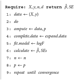
Algorithm 1. Validation algorithm for the LogF method.

From Table 1, the first column of the table represents the sample size (n), the second column represents, the proportion of the missigness, the parameter of interest, and the bias reduction method, while the last two columns show, the estimated parameter $(\widehat{\beta })$, the standard error of the estimated parameters. The simulation results show that the Ibrahim's method over estimates the model parameters in most of the scenarios, but as the sample size increases some estimates tend to get closer to the true values. For example, the true parameter for variable x₂ is β₂ = 0.7, while the results from the Ibrahim's method were {0.8349, 1.0002, 0.4185, 0.6875}, implying better performance with increased sample size. This tendency is consistent throughout the various simulations conducted, except for very few cases, which may be attributed to the randomness used to generate the dataset and the proportion of the missing data.

TABLE 1

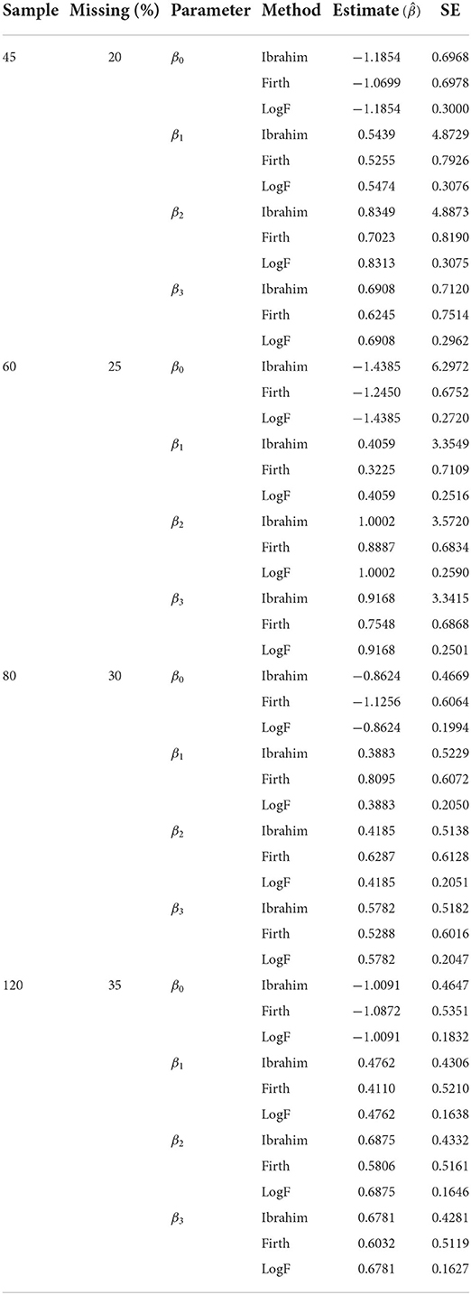
Table 1. Validation of the LogF method using standard errors.

Further, for the small sample size the Firth method performed better, and this may be mainly attributed to its ability to solve the separation problem in the smaller samples. For example, with n = 45, we found that the corresponding estimate for x₂ was (0.7023) which is very close to the true estimate (β₂ = 0.7), however with n = 45, the same estimate for x₂ was (0.5806). The estimates obtained from our proposed method, the logF were in many cases closer to the true estimates, especially as the sample size and proportion of missingness increased. For instance, estimates for β₂ = 0.7 as the sample size and missingness increase were $\widehat{{\beta }_2}=\left\{0.8313,1.002,0.4185,0.6875\right\}$. The ability to outperform other methods under situations when the sample size increases is a strong attribute toward applicability of our method, since this represents the real world situations.

Several methods have been developed to compute standard errors of parameter estimates by using the EM algorithm. Some methods are known to be specific on the incomplete data problem [29], whereas others are more general [20]. In Louis' method, the observed information matrix is computed on the last iteration of the EM procedure using only the complete-data gradient and second derivative matrix. The observed information matrix needs to be inverted in order to obtain estimates of the covariance matrix. However, since the Louis' method for estimating standard errors is quite technical [30] and given the fact that the purpose of our simulation is simply to validate the proposed method, we opted for a faster, and reliable alternative of examining the SEs of the estimates. The alternative approach uses the negative of the second derivative matrix of the incomplete-data log-likelihood as an estimate of the information matrix, which can be inverted in order to obtain an estimate of the covariance matrix. Overall, the smallest standard errors were observed from the proposed logF penalized method, thus demonstrating its superiority over both Ibrahim and Firth methods in reducing bias under the MAR assumption.

4.2. Application of bias reduction with LogF(1,1) prior on the COVID-19 data

In this section, we validated our method based on a real-life data problem for determining the potential risk factors of COVID-19 patient being admitted to the Intensive Care Unit (ICU). Thus, we compare between our proposed method logF against the proposed by Ibrahim and Firth when data are MAR. The survey data were collected between January 2020 and June 2020 from the Royal Hospital in the Sultanate of Oman [18]. The study aimed to assess the risk factors associated with admissions to the intensive care unit, ICU for the COVID-19 hospitalized patients. Details of this data were described in the section for the motivation of this study. As presented in Figure 1, the covariates include; having conjuctivitis, being unconscious and having a neurological problem. The response variable was whether the patient was admitted to an intensive care unit or not. In the study, the proportions of missing data for each explanatory variable were as follows; conjuctivitis (34%), unconscious (2%), and neurological (4%). We explored by fitting a logistic model for the ICU admission and compared results with the complete case analysis (CCA). The main objective of the study was to obtain estimates for the model based on our proposed method, the logF penalty, and to compare the estimates with those obtained from Ibrahim and Firth methods, by examining their standard errors. The results are summarized in Table 2.

TABLE 2

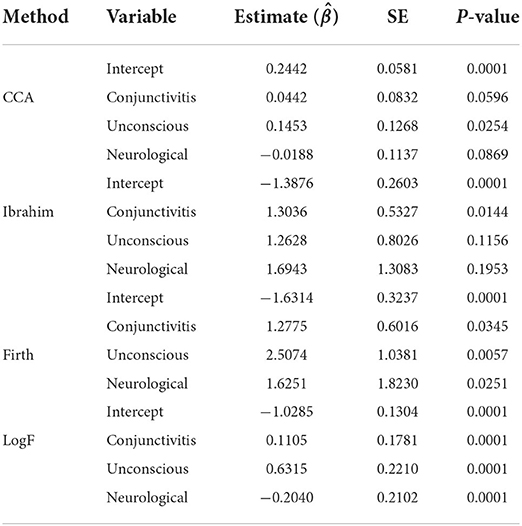
Table 2. Performance of LogF against the Ibrahim and Firth methods.

From Table 2, it can be observed that, the parameter estimates under all the methods; CCA, Ibrahim, Firth, and logF give different values of the coefficients. They show that lowest standard errors are achieved for the proposed method, implying that narrower confidence intervals for all the three covariates can be obtained using the proposed method, hence reduced bias. For the Ibrahim's method, every unit increase in conjuctivitis, being unconscious and having a neurological there is an increase in the log-odds of patient's ICU admission by 1.3036, 1.2628, and 1.6943, respectively. Whereas, using the Firth's method, for every unit increase in conjuctivitis, being unconscious and having a neurological, the log-odds of ICU admission would increase by 1.2775, 2.5074, and 1.6251, respectively.

Figure 2 demonstrates the variation of estimated parameters $(\widehat{\beta })$, their confidence intervals computed from the SEs, the probability values and the different methods of estimation. Clearly, the parameter estimates were smallest under the logF method of bias reduction as compared to the other methods. Conceptually, under the logF method of bias reduction, all variables were statistically significant, a distinct result from other comparable methods of bias reduction, besides the ones derived from the Firth method. Moreover, results of the complete case analysis (CCA) and Ibrahim's method each indicate only one different significant parameter, smaller SEs under the CCA than the Ibrahim's method. Interestingly, the SEs for the Intercept were smallest under the CCA, followed by the LogF method, possibly because CCA analyses only complete data, yet LogF first imputes before parameter estimation.

FIGURE 2

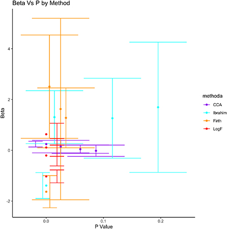
Figure 2. Validation of LogF against CCA, Ibrahim, and Firth methods.

5. Discussion

In this study, we have demonstrated the importance of bias reduction of estimates for the logistic model under the missing at random mechanism. We conducted model validation studies using both simulation and real life COVID-19 patient data analysis and presented summary statistical results. Our novel method for bias reduction is robust as it relies on the penalization theory of the likelihood function to achieve the efficiency in the parameter estimates for the missing at random data mechanism [6, 31–33]. The fact that we penalized the log-likelihood function by the LogF(1, 1) prior and then, derived the closed form of the bias using the Cox and Snell's equation [19] shows how broadbased the novel method is. Besides, the information matrix was derived using the Louis' method [20, 34, 35]. The simulation studies conducted show results, which reveal that irrespective of the sample size, the proposed method based on the LogF penalty provides more accurate estimates, characterized by lower standard errors of the model estimates. Furthermore, the results from real life COVID-19 data also support the conclusion that the proposed LogF outperforms both the Firth and Ibrahim methods. These results from the application agree with the clinician's theory that admission to ICU for the COVID-19 patient is significantly explained by the three factors that is, conjuctivitis, unconsciousness and having a neurological condition [36, 37]. We also note that using the complete case analysis alone in modeling may lead to incorrect logit model, as it may be determined that a predictor is not significant, when actually the reverse is true or otherwise.

6. Conclusion

In this study, we have proposed a bias reduction method for the logit model when data are missing at random. Its theoretical aspects have been validated using simulation and real life data problems. The method is based on penalization of the log-likelihood function with Log-F(1,1) penalty chosen for its almost near to normal distribution for the missing at random mechanism. Its related information matrix and the exact form of the bias for that model were derived theoretically. The method is novel, it can efficiently be used to estimate logit model parameters when data are MAR. The results from statistical validation studies show better performance for the novel method when the categorical covariate data are missing at random than other methods. Therefore, we can conclude that the new method shows greater superiority in reducing the bias under MAR in contrast to the current bias reduction methods in estimated parameters by Ibrahim and Firth. The approach yields more efficient estimates in contrast to the existing classical methods, especially for larger sample sizes and missingness proportions. We recommend further research on bias reduction in parameters under other missing data mechanisms for other generalized linear models. The other research consideration is parameter estimation when the model covariates are not all categorical.

Data availability statement

The original contributions presented in the study are included in the article/supplementary material, further inquiries can be directed to the corresponding author/s.

Author contributions

MA-S conceptualized the study and contributed to the writing. MA-S and RW contributed substantially to the writing. All authors contributed to the article and approved the submitted version.

Conflict of interest

The authors declare that the research was conducted in the absence of any commercial or financial relationships that could be construed as a potential conflict of interest.

Publisher's note

All claims expressed in this article are solely those of the authors and do not necessarily represent those of their affiliated organizations, or those of the publisher, the editors and the reviewers. Any product that may be evaluated in this article, or claim that may be made by its manufacturer, is not guaranteed or endorsed by the publisher.

References

1. Santi F, Dickson MM, Giuliani D, Arbia G, Espa G. Reduced-bias estimation of spatial autoregressive models with incompletely geocoded data. Comput Stat. (2021) 36:2563–90. doi: 10.1007/s00180-021-01090-7

CrossRef Full Text | Google Scholar

2. Lee SM, Pho KH, Li CS. Validation likelihood estimation method for a zero-inflated Bernoulli regression model with missing covariates. J Stat Plann Infer. (2021) 457:105–27. doi: 10.1016/j.jspi.2021.01.005

CrossRef Full Text | Google Scholar

3. Jin J, Ma T, Dai J, Liu S. Penalized weighted composite quantile regression for partially linear varying coefficient models with missing covariates. Comput Stat. (2021) 36:541–75. doi: 10.1007/s00180-020-01012-z

CrossRef Full Text | Google Scholar

4. Özkale MR, Lemeshow S, Sturdivant R. Logistic regression diagnostics in ridge regression. Comput Stat. (2018) 33:563–93. doi: 10.1007/s00180-017-0755-x

CrossRef Full Text | Google Scholar

5. Chen YJ, DeMets DL, Gordon Lan K. Increasing the sample size when the unblinded interim result is promising. Stat Med. (2004) 23:1023–38. doi: 10.1002/sim.1688

PubMed Abstract | CrossRef Full Text | Google Scholar

6. Firth D. Bias reduction of maximum likelihood estimates. Biometrika. (1993) 80:27–38. doi: 10.1093/biomet/80.1.27

CrossRef Full Text | Google Scholar

7. Heinze G. A comparative investigation of methods for logistic regression with separated or nearly separated data. Stat Med. (2006) 25:4216–26. doi: 10.1002/sim.2687

PubMed Abstract | CrossRef Full Text | Google Scholar

8. Gaucher S, Klopp O. Maximum likelihood estimation of sparse networks with missing observations. J Stat Plann Infer. (2021) 215:299–329. doi: 10.1016/j.jspi.2021.04.003

CrossRef Full Text | Google Scholar

9. Kosmidis I, Firth D. A generic algorithm for reducing bias in parametric estimation. Electron J Stat. (2010) 4:1097–112. doi: 10.1214/10-EJS579

CrossRef Full Text | Google Scholar

10. Rainey C. Dealing with separation in logistic regression models. Polit Anal. (2016) 24:339–55. doi: 10.1093/pan/mpw014

CrossRef Full Text | Google Scholar

11. Little RJ, Rubin DB. Statistical Analysis With Missing Data. Vol. 793. Hoboken, NJ: John Wiley & Sons (2019). doi: 10.1002/9781119482260

CrossRef Full Text | Google Scholar

12. Ibrahim JG. Incomplete data in generalized linear models. J Am Stat Assoc. (1990) 85:765–9. doi: 10.1080/01621459.1990.10474938

PubMed Abstract | CrossRef Full Text | Google Scholar

13. Ibrahim JG, Lipsitz SR. Parameter estimation from incomplete data in binomial regression when the missing data mechanism is nonignorable. Biometrics. (1996) 52:1071–8. doi: 10.2307/2533068

PubMed Abstract | CrossRef Full Text | Google Scholar

14. Das U, Maiti T, Pradhan V. Bias correction in logistic regression with missing categorical covariates. J Stat Plann Infer. (2010) 140:2478–85. doi: 10.1016/j.jspi.2010.02.018

CrossRef Full Text | Google Scholar

15. Maity AK, Pradhan V, Das U. Bias reduction in logistic regression with missing responses when the missing data mechanism is nonignorable. Am Stat. (2018) 73:340–9. doi: 10.1080/00031305.2017.1407359

CrossRef Full Text | Google Scholar

16. Karl AT, Zimmerman DL. A diagnostic for bias in linear mixed model estimators induced by dependence between the random effects and the corresponding model matrix. J Stat Plann Infer. (2021) 211:107–18. doi: 10.1016/j.jspi.2020.06.004

CrossRef Full Text | Google Scholar

17. Greenland S, Mansournia MA. Penalization, bias reduction, and default priors in logistic and related categorical and survival regressions. Stat Med. (2015) 34:3133–43. doi: 10.1002/sim.6537

PubMed Abstract | CrossRef Full Text | Google Scholar

18. Al Awaidy ST, Khamis F, Mahomed O, Wesonga R, Al Shuabi M, Al Shabibi NS, et al. Epidemiological risk factors for acquiring severe COVID-19; prospective cohort study. Oman Med J. (2021) 36:e301. doi: 10.5001/omj.2021.127

PubMed Abstract | CrossRef Full Text | Google Scholar

19. Cox DR, Snell EJ. A general definition of residuals. J R Stat Soc Ser B. (1968) 30:248–65. doi: 10.1111/j.2517-6161.1968.tb00724.x

CrossRef Full Text | Google Scholar

20. Louis TA. Finding the observed information matrix when using the EM algorithm. J R Stat Soc Ser B. (1982) 44:226–33. doi: 10.1111/j.2517-6161.1982.tb01203.x

CrossRef Full Text | Google Scholar

21. Rubin DB. Inference and missing data. Biometrika. (1976) 63:581–92. doi: 10.1093/biomet/63.3.581

CrossRef Full Text | Google Scholar

22. Kim JK, Shao J. Statistical Methods for Handling Incomplete Data. Boca Raton, FL: CRC Press (2013). doi: 10.1201/b13981

CrossRef Full Text | Google Scholar

23. Li W, Yang S, Han P. Robust estimation for moment condition models with data missing not at random. J Stat Plann Infer. (2020) 207:246–54. doi: 10.1016/j.jspi.2020.01.001

CrossRef Full Text | Google Scholar

24. Chen TH, Chatterjee N, Landi MT, Shi J. A penalized regression framework for building polygenic risk models based on summary statistics from genome-wide association studies and incorporating external information. J Am Stat Assoc. (2021) 116:133–43. doi: 10.1080/01621459.2020.1764849

PubMed Abstract | CrossRef Full Text | Google Scholar

25. Prentice RL. Discrimination among some parametric models. Biometrika. (1975) 62:607–14. doi: 10.1093/biomet/62.3.607

CrossRef Full Text | Google Scholar

26. Kalbfleisch JD, Prentice RL. The Statistical Analysis of Failure Time Data. John Wiley & Sons (2011).

PubMed Abstract | Google Scholar

27. Brown BW, Spears FM, Levy LB. The log F: a distribution for all seasons. Comput Stat. (2002) 17:47–58. doi: 10.1007/s001800200098

CrossRef Full Text | Google Scholar

28. Aroian LA. A study of RA Fisher's z distribution and the related F distribution. Ann Math Stat. (1941) 12:429–48.

Google Scholar

29. Baker SG. A simple method for computing the observed information matrix when using the EM algorithm with categorical data. J Comput Graph Stat. (1992) 1:63–76. doi: 10.1080/10618600.1992.10474576

CrossRef Full Text | Google Scholar

30. Kang SM, Rafiq A, Kwun YC. A new second-order iteration method for solving nonlinear equations. In:Lee G, , editor. Abstract and Applied Analysis. Vol. 2013. London: Hindawi (2013). doi: 10.1155/2013/487062

PubMed Abstract | CrossRef Full Text | Google Scholar

31. Bindele HF, Abebe A, Meyer NK. Robust confidence regions for the semi-parametric regression model with responses missing at random. Statistics. (2018) 52:885–900. doi: 10.1080/02331888.2018.1467419

CrossRef Full Text | Google Scholar

32. Zou YY, Liang HY. Wavelet estimation of density for censored data with censoring indicator missing at random. Statistics. (2017) 51:1214–37. doi: 10.1080/02331888.2017.1336170

CrossRef Full Text | Google Scholar

33. Wang Q. Probability density estimation with data missing at random when covariables are present. J Stat Plann Infer. (2008) 138:568–87. doi: 10.1016/j.jspi.2006.10.017

CrossRef Full Text | Google Scholar

34. Le Cessie S, Van Houwelingen JC. Ridge estimators in logistic regression. J R Stat Soc Ser C. (1992) 41:191–201. doi: 10.2307/2347628

CrossRef Full Text | Google Scholar

35. Cole SR, Chu H, Greenland S. Maximum likelihood, profile likelihood, and penalized likelihood: a primer. Am J Epidemiol. (2014) 179:252–60. doi: 10.1093/aje/kwt245

PubMed Abstract | CrossRef Full Text | Google Scholar

36. Gallo Marin B, Aghagoli G, Lavine K, Yang L, Siff EJ, Chiang SS, et al. Predictors of COVID-19 severity: a literature review. Rev Med Virol. (2021) 31:1–10. doi: 10.1002/rmv.2146

PubMed Abstract | CrossRef Full Text | Google Scholar

37. Elemam NM, Hammoudeh S, Salameh L, Mahboub B, Alsafar H, Talaat IM, et al. Identifying immunological and clinical predictors of COVID-19 severity and sequelae by mathematical modeling. Front Immunol. (2022) 13:865845. doi: 10.3389/fimmu.2022.865845

PubMed Abstract | CrossRef Full Text | Google Scholar