Numerical treatment of singularly perturbed unsteady Burger-Huxley equation

1. Introduction

Singular perturbed non-linear parabolic partial differential equations have many applications in real life scenarios. A good example of singularly perturbed nonlinear differential equations is the mathematical model for the prototype model used to describe the interaction between non-linear convection effects, reaction mechanisms, and diffusion transport. This equation has many intriguing phenomena such as bursting oscillation [1], interspike [2], population genetics [3], bifurcation, and chaos [4]. Several membrane models based on the dynamics of potassium and sodium ion fluxes were found in Lewis et al. [5].

Many researchers have made efforts to construct analytical and numerical methods for Burger equations, for instance, Ismail et al. [6], Javidi et al. [7], Estevez [8], Krisnangkura et al. [9], Satsuma et al. [10], Wang et al. [11], Hashim et al. [12, 13], Khattak [14], Krisnangkur et al. [9], Mohammadi [15], Sari et al. [16], Appadu et al. [17, 18], and Appadu and Tijani [19], and references therein. A Burger-Huxley equation in which the highest order derivative is multiplied by a perturbation parameter ε (0 < ε << 1) is termed the singularly perturbed Burger-Huxley equation (SPBHE). Due to the presence of the perturbation parameter and the nonlinearity in the problem, finding their solutions are tedious task. For instance, due to the presence of the perturbation parameter, the solution exposes boundary/shrill interior layer(s), and it is not easy to find a stable numerical approximation. The methods suggested in Ismail et al. [6], Javidi and Golbabai [7], Estevez [8], Krisnangkura et al. [9], Satsuma et al. [10], Wang et al. [11], Hashim et al. [12, 13], Khattak [14], Mohammadi [15], and Sari and Gürarslan [16] and other standard numerical methods on a uniform mesh is insufficient to approximate the SPBHE. Thus, to resolve this drawback, the fitting approaches are competitive computational techniques to overcome the limitations of classical numerical methods. Kaushik and Sharma [20] presented a uniformly convergent finite difference method (FDM) for the problem Equation (1). Gupta and Kadalbajoo [21] developed a numerical method that comprises an implicit-Euler method and a monotone hybrid finite difference operator with a Shishkin mesh type for the problem Equation (1). A robust numerical method that consists of a backward-Euler method and an upwind FDM on an adaptive nonuniform grid for Equation (1) is suggested by Liu et al. [22]. Kabato and Duressa [23] and Jima et al. [24] considered a similar problem as in Liu et al. [22] and proposed a parameter uniform numerical method based on fitted operator techniques. Kehinde et al. [25] developed a fitted operator FDM for the two-dimensional semilinear singularly perturbed convection-diffusion problem.

However, there has been little development in the numerical treatment of the problem Equation (1). This work aims to develop and analyze an ε, which is a uniformly convergent numerical method for solving the problem Equation (1). First, the nonlinear terms are linearized by using the Newton-Raphson-Kantorovich approximation method. Then, we approximate the resulting singularly perturbed parabolic convection-diffusion equations using the implicit Euler method for the time derivative and fitted the exponential spline method for the space derivative on a uniform step length. Finally, to enhance the order of convergence in the time variable, the Richardson extrapolation technique is applied to the temporal variable. The novelty of the presented method, unlike Shishkin and Bakhvalov mesh types, does not require a priori information about the location and width of the boundary layer.

2. Continuous problem

On the domain ϒ = χ_z × χ_t = (0, 1) × (0, T], we consider singularly perturbed Burger-Huxley equation of the form

$\begin{array}{ll}\{\begin{array}{l}{\pounds }_{\epsilon }\Im (z,t)=\frac{\partial \Im }{\partial t}-\epsilon \frac{{\partial }^2\Im }{\partial z^2}+\alpha \Im \frac{\partial \Im }{\partial z}-\theta (1-\Im )(\Im -\lambda )=0,(z,t)\in \Upsilon ,\\ \Im (z,0)={\Im }_0(z),z\in {\overline{\chi }}_z,\\ \Im (0,t)={\Theta }_0(t),\Im (1,t)={\Theta }_1(t),t\in {\chi }_t,\end{array}& (1)\end{array}$

Where 0 < ε ≪ 1 is a singular perturbation parameter and α ≥ 1, θ ≥ 0, and λ ∈ (0, 1). The functions Θ₀(t), Θ₁(t), and $\Im$₀(z) are assumed to be sufficiently smooth, bounded, and independent of ε.

Lemma 2.1 (Maximum principle). If $\Im \in C^{2,1}(\overline{\Upsilon })$, $\Im$|_∂ϒ ≥ 0, and £_εℑ|_ϒ ≥ 0, then $\Im {|}_{\overline{\Upsilon }}\ge 0$.

Proof. See Gupta and Kadalbajoo [21].

An immediate consequence of Lemma 2.1 for the solution of problem Equation (1) resulted in Lemma 2.2.

Lemma 2.2 (Stability estimate). Let $\Im$(z, t) be the solution of problem Equation (1), then we have,

$\begin{array}{l}\left|\right|\Im |{|}_{\overline{\Upsilon }}\le T|\left|{\Im }_0\right|{|}_{{\Gamma }_i}+\left|\right|\Im |{|}_{\partial \Upsilon }.\end{array}$

Proof. See Gupta and Kadalbajoo [21].

3. Formulation of the numerical scheme

3.1. Quasi-linearization

The Equation (1) is rewritten as

$\begin{array}{ll}\{\begin{array}{l}{\pounds }_{\epsilon }\Im (z,t)=\left(\frac{\partial \Im }{\partial t}-\epsilon \frac{{\partial }^2\Im }{\partial z^2}\right)(z,t)=\zeta (z,t,\Im (z,t),{\Im }_z(z,t)),(z,t)\in \Upsilon ,\\ \Im (z,0)={\Im }_0(z),z\in {\overline{\chi }}_z,\\ \Im (0,t)={\Theta }_0(t),\Im (1,t)={\Theta }_1(t),t\in (0,T],\end{array}& (2)\end{array}$

Where $\zeta (z,t,\Im (z,t),{\Im }_z(z,t))=-\alpha \Im \frac{\partial \Im }{\partial z}+\theta (1-\Im )(\Im -\lambda )$ is the non-linear function of z, t, $\Im$(z, t), $\Im$_z(z, t).

To linearize the semi-linear term of Equation (1), we choose the reasonable initial approximation for the function $\Im$(z, t) in the term ζ(z, t, $\Im$(z, t), $\Im$_z(z, t)) and denote it as $\Im$⁰(z, t) that satisfy both initial and boundary conditions which are obtained by the separation of variables method of the homogeneous part of the problem under consideration and is given by Kabeto and Duressa [23].

$\begin{array}{ll}{\Im }^0(z,t)={\Im }_0(z)exp(-{\pi }^{2}t)& (3)\end{array}$

Thus, the nonlinear term ζ(z, t, $\Im$(z, t), $\Im$_z(z, t)) of Equation (2) can be linearized by applying the Newton-Raphson- Kantorovich approximation approach as

$\begin{array}{ll}\begin{array}{l}\zeta (z,t,{\Im }^{(k+1)}(z,t),{\Im }_z^{(k+1)}(z,t))\cong \zeta (z,t,{\Im }^{(k)}(z,t),{\Im }_z^{(k)}(z,t))+\\ ({\Im }^{(k+1)}(z,t)-{\Im }^{(k)}(z,t)){\zeta }_{\Im }|(\Im ,t,{\Im }^{(k)}(z,t),{\Im }_z^{(k)}(z,t))+\\ ({\Im }_z^{(k+1)}(z,t)-{\Im }_z^{(k)}(\Im ,t)){\zeta }_{{\Im }_z}|(z,t,{\Im }^{(k)}(z,t),{\Im }_z^{(k)}(z,t))+\cdots ,\end{array}& (4)\end{array}$

Where ${\left\{{\Im }^{(k)}\right\}}_{k=0}^{\infty }$ are a sequence of approximate solutions of ζ(z, t, $\Im$(z, t), $\Im$_z(z, t)).

Substituting Equation (4) into Equation (2), we have

$\begin{array}{ll}\{\begin{array}{l}{\pounds }_{\epsilon }{\Im }^{(k+1)}(z,t)={\Im }_t^{(k+1)}(z,t)-\epsilon {\Im }_{zz}^{(k+1)}(z,t)\\ +\varpi (z,t){\Im }_z^{(k+1)}(z,t)+q(z,t){\Im }^{(k+1)}(z,t)\\ =v(z,t),\\ {\Im }^{(k+1)}(z,0)={\Im }_0(z),z\in {\overline{\chi }}_z,\\ {\Im }^{(k+1)}(0,t)={\Theta }_0(t),t\in {\overline{\chi }}_t,\\ {\Im }^{(k+1)}(1,t)={\Theta }_1(t),t\in {\overline{\chi }}_t,\end{array}& (5)\end{array}$

where

$\begin{array}{l}\begin{array}{l}\varpi (z,t)=-{\zeta }_{u_z}|(z,t,{\Im }^{(k)}(z,t),{\Im }_z^{(k)}(z,t)),\\ q(z,t)=-{\zeta }_{\Im }|(z,t,{\Im }^{(k)}(z,t),{\Im }_z^{(k)}(z,t)),\\ v(z,t)=\zeta (z,t,{\Im }^{(k)}(z,t),{\Im }_z^{(k)}(z,t))\\ -{\Im }^{(k)}{\zeta }_{\Im }|(z,t,{\Im }^{(k)}(z,t),{\Im }_z^{(k)}(z,t))\\ -{\Im }_z^{(k)}{\zeta }_{{\Im }_z}|(z,t,{\Im }^{(k)}(z,t),{\Im }_z^{(k)}(z,t)).\end{array}\end{array}$

3.2. Temporal semi-discretization

We define the uniform mesh for the domain χ_t as ${\chi }_t={\Upsilon }_{\tau }^M=\left\{t_j=j\tau ,\forall j=0,2,3,\cdots ,M,\tau =1/M\right\}$ and we approximated the temporal derivative term of Equation (5) using implicit Euler method, which gives

$\begin{array}{ll}\{\begin{array}{l}(1+\tau {\pounds }_{\epsilon }^M){\widehat{\Im }}^{k+1}(z,t_{j+1})=-\epsilon {\widehat{\Im }}_{zz}^{k+1}(z,t_{j+1})\\ +\varpi (z,t_{j+1}){\widehat{\Im }}_z^{k+1}(z,t_{j+1})\\ +q(z,t_{j+1}){\widehat{\Im }}^{k+1}(z,t_{j+1})-v(z,t_{j+1})\\ ={\widehat{\Im }}^{k+1}(z,t_j),\\ {\widehat{\Im }}^{k+1}(z,0)={\widehat{\Im }}_0^{k+1}(z),z\in {\overline{\chi }}_z,\\ {\widehat{\Im }}^{k+1}(0,t_{j+1})={\Theta }_0(t_{j+1}),0\le j\le M-1,\\ {\widehat{\Im }}^{k+1}(1,t_{j+1})={\Theta }_1(t_{j+1}),0\le j\le M-1.\end{array}& (6)\end{array}$

Since $\varpi (z,t_{j+1})\ge {\varpi }^{*}>0$ and $q(z,t_{j+1})\ge q^{*}>0,z\in {\overline{\chi }}_z$ Equation (6) exhibits boundary located at z = 1 and admits a unique solution.

Lemma 3.1 (Local Error Estimate). In the solution of Equation (6), the local truncation error estimate is bounded by

$\begin{array}{l}\left|\right|LT{E}_{j+1}|{|}_{\infty }\le C^{*}{(\tau )}^2,\end{array}$

Where C^* is a positive constant independent of ε and τ.

Proof. On applying Taylor's series expansion on ${\widehat{\Im }}^{k+1}(z,t_{j+1})$ yields

$\begin{array}{l}\begin{array}{l}{\widehat{\Im }}^{k+1}(z,t_{j+1})={\widehat{\Im }}^{k+1}(z,t_j)+\tau {\widehat{\Im }}_t^{k+1}(z,t_j)+O({(\tau )}^2).\end{array}\end{array}$

This implies

$\begin{array}{ll}\frac{{\widehat{\Im }}^{k+1}(z,t_{j+1})-{\widehat{\Im }}^{k+1}(z,t_j)}{\tau }={\widehat{\Im }}_t^{k+1}(z,t_j)+O(\tau ).& (7)\end{array}$

Substituting Equation (5) into Equation (7) we have

$\begin{array}{ll}\begin{array}{l}\frac{{\widehat{\Im }}^{k+1}(z,t_{j+1})-{\widehat{\Im }}^{k+1}(z,t_j)}{\tau }\\ =-(-\epsilon {\widehat{\Im }}_{zz}^{k+1}(z,t_j)+\varpi (z,t_j){\widehat{\Im }}_z^{k+1}(z,t_j)\\ +q(z,t_j){\widehat{\Im }}^{k+1}(z,t_j)-v(z,t_j))+O(\tau )\\ \Rightarrow (1+\tau {\pounds }_{\epsilon }^M){\widehat{\Im }}^{k+1}(z,t_{j+1})-\tau v(z,t_j)+{\widehat{\Im }}^{k+1}(z,t_j)=O{(\tau )}^2).\end{array}& (8)\end{array}$

Subtracting Equation (6) from Equation (8), and the local truncation error $LT{E}_{j+1}={\widehat{\Im }}^{k+1}(z,t_{j+1})-{\widehat{\Im }}^{k+1}(z,t_{j+1})$ at (j + 1)th is the solution of a BVP

$\begin{array}{ll}\begin{array}{l}(1+\tau {\pounds }_{\epsilon }^M)LT{E}_{j+1}=O({(\tau )}^2),LT{E}_{j+1}(0)=0=LT{E}_{j+1}(1).\end{array}& (9)\end{array}$

Hence, applying the maximum principle on the operator gives

$\begin{array}{l}\left|\right|LT{E}_{j+1}|{|}_{\infty }\le C^{*}{(\tau )}^2.\end{array}$

Lemma 3.2. [Global Error Estimate (GEE)] The GEE in the temporal direction of Equation (6) is given by

$\begin{array}{l}\left|\right|E_j|{|}_{\infty }\le C(\tau ),\forall j\le T/\tau .\end{array}$

Proof. Using Lemma 3.1, we obtain the following GEE at (j)th time step

$\begin{array}{l}\begin{array}{l}\left|\right|E_j|{|}_{\infty }=\left|\right|{\displaystyle {\sum }_{i=1}^j}LT{E}_i|{|}_{\infty },j\le T/\tau \\ \le \left|\right|LT{E}_1|{|}_{\infty }+|\left|LT{E}_2\right|{|}_{\infty }+\left|\right|LT{E}_3|{|}_{\infty }+\cdots +|\left|e_j\right|{|}_{\infty }\\ \le c_{1}j{(\tau )}^2(\text{by Lemma }3.1)\\ \le c_1(j\tau )(\tau )\\ \le c_{1}T(\tau )(j\tau \le T)\\ \le C(\tau ),\end{array}\end{array}$

Where c₁, C are positive constants independent of ε and τ.

Lemma 3.3. The solution ${\widehat{\Im }}^{k+1}(z)$ of the Equation (6) is bounded by

$\begin{array}{l}\left|\right|\frac{{\partial }^m{\widehat{\Im }}^{k+1}(z,t_{j+1})}{\partial z^m}|{|}_{{\overline{\chi }}_z}\le C\left(1+{\epsilon }^{-m}exp\left(\frac{-({\varpi }^{*}(1-z))}{\epsilon }\right)\right),\\ 0\le m\le 4.\end{array}$

Proof. See Gupta et al. [21].

3.2.1. Spatial semi-discretization

We define the uniform mesh for the space domain [0, 1] as

$\begin{array}{l}{\Upsilon }_{\ell }^N=\left\{z_i=i\ell ,\forall i=1,2,3,\cdots ,N,z_0=0,z_N=1,\ell =1/N\right\}.\end{array}$

Equation (6) can be rewritten as

$\begin{array}{ll}\begin{array}{l}-\epsilon {\widehat{\Im }}_{zz}^{k+1}(z,t_{j+1})+\varpi (z,t_{j+1}){\widehat{\Im }}_z^{k+1}(z,t_{j+1})\\ +r(z,t_{j+1}){\widehat{\Im }}^{k+1}(z,t_{j+1})=\phi (z,t_{j+1}),\\ \widehat{\Im }(0,t_{j+1})={\Theta }_0(t_{j+1}),\widehat{\Im }(1,t_{j+1})={\Theta }_1(t_{j+1}),z\in {\chi }_z,\\ 0\le j\le M-1,\end{array}& (10)\end{array}$

Where $r(z,t_{j+1})=\left(q(z,t_{j+1})+\frac{1}{\tau }\right)$ and $\phi (z,t_{j+1})=v(z,t_{j+1})+\frac{{\widehat{\Im }}^{k+1}(z,t_j)}{\tau }$.

For spatial discretization of Equation (10), we use an exponential cubic spline method.

The approximation solution ${\widehat{\Im }}_i^{j+1}$ of Equation (10) obtained by the segment S_△(z) passing through the points $\left(z_i,{\widehat{\Im }}_i^{j+1}\right)$ and $\left(z_{i+1},{\widehat{\Im }}_{i+1}^{j+1}\right)$. Each mixed spline segment $S_{△}^{j+1}(z)$ has the form [26].

$\begin{array}{ll}{S}_{△}^{j+1}(z)=A_i{e}^{\psi (z-z_i)}+B_i{e}^{-\psi (z-z_i)}+C_i(z-z_i)+D_i,0\le i\le N,& (11)\end{array}$

Where A_i, B_i, C_i, and D_i are constants and ψ ≠ 0 is a free parameter that is used to enhance the accuracy of the method. To find the values of A_i, B_i, C_i, and D_i in Equation (11), we denote

$\begin{array}{ll}\begin{array}{l}{S}_{△}^{j+1}(z_i)={\widehat{\Im }}_i^{j+1},S_{△}^{j+1}(z_{i+1})={\widehat{\Im }}_{i+1}^{j+1},\\ \frac{d^2{S}_{△}^{j+1}(z_i)}{d{z}^2}={\Xi }_i,\frac{d^2{S}_{△}^{j+1}(z_{i+1})}{d{z}^2}={\Xi }_{i+1}.\end{array}& (12)\end{array}$

Differentiating twice both sides of Equation (11), we get

$\begin{array}{ll}\frac{d^2{S}_{△}^{j+1}(z)}{d{z}^2}={\psi }^2\left(A_i{e}^{\psi (z-z_i)}+B_i{e}^{-\psi (z-z_i)}\right).& (13)\end{array}$

Using the relation in Equation (12) into Equation (13) at z = z_i, we get

$\begin{array}{l}\frac{d^2{S}_{△}^{j+1}(z_i)}{d{z}^2}={\Xi }_i={\psi }^2(A_i+B_i)\end{array}$

and it yields

$\begin{array}{ll}{A}_i=\frac{{\ell }^2{\Xi }_i}{{\varrho }^2}-B_i.& (14)\end{array}$

Where ϱ = ψℓ and i = 0, 1, 2, ⋯ , N.

Again substituting Equation (12) into Equation (13) at z = z_i+1, we obtain

$\begin{array}{l}\frac{d^2{S}_{△}^{j+1}(z_{i+1})}{d{z}^2}={\Xi }_{i+1}={\psi }^2\left(A_i{e}^{\varrho }+B_i{e}^{-\varrho }\right)\end{array}$

and it gives

$\begin{array}{ll}{A}_i=e^{-\varrho }\left(\frac{{\ell }^2{\Xi }_{i+1}}{{\varrho }^2}\right)-B_i{e}^{-2\varrho }.& (15)\end{array}$

From Equations (14) and (15), we have

$\begin{array}{ll}{A}_i=\frac{{\ell }^2({\Xi }_{i+1}-{\Xi }_i{e}^{-\varrho })}{2{\varrho }^{2}sinh(\varrho )}\text{ and }{B}_i=\frac{{\ell }^2({\Xi }_i{e}^{\varrho }-{\Xi }_{i+1})}{2{\varrho }^{2}sinh(\varrho )}.& (16)\end{array}$

Substituting Equation (12) into Equation (11) at z = z_i and z = z_i+1, we obtain

$\begin{array}{l}{S}_{△}^{j+1}(z_i)={\widehat{\Im }}_i^{j+1}=A_i+B_i+D_i,\text{ and }{S}_{△}^{j+1}(z_{i+1})={\widehat{\Im }}_{i+1}^{j+1}\\ =A_i{e}^{\varrho }+B_i{e}^{-\varrho }+C_i\ell +D_i,\end{array}$

which implies

$\begin{array}{l}{C}_i=\frac{\left({\widehat{\Im }}_{i+1}^{j+1}-{\widehat{\Im }}_i^{j+1}\right)}{\ell }-\frac{\ell \left({\Xi }_{i+1}-{\Xi }_i\right)}{{\varrho }^2}\text{ and}\\ D_i={\widehat{\Im }}_i^{j+1}-\left(\frac{{\ell }^2}{{\varrho }^2}{\Xi }_i\right).& (17)\end{array}$

The first derivative continuity condition at z = z_i, that is S_△−1(z_i) = S_△(z_i) gives

$\begin{array}{l}{\ell }^2\left({\omega }_1{\Xi }_{i-1}+2{\omega }_2{\Xi }_i+{\omega }_1{\Xi }_{i+1}\right)=\left({\widehat{\Im }}_{i-1}^{j+1}-2{\widehat{\Im }}_i^{j+1}+{\widehat{\Im }}_{i+1}^{j+1}\right),\\ i=1,2,\cdots ,N-1,& (18)\end{array}$

where

$\begin{array}{l}{\omega }_1=\left(\frac{sinh(\varrho )-\varrho }{{\varrho }^{2}sinh(\varrho )}\right)\text{ and }{\omega }_2=\left(\frac{2\varrho cosh(\varrho )-2sinh(\varrho )}{{\varrho }^{2}sinh(\varrho )}\right).\end{array}$

Now from Equation (10), we have

$\begin{array}{ll}\{\begin{array}{l}\epsilon {\Xi }_{i-1}={\varpi }^{j+1}(z_{i-1}){\widehat{\Im }}_z^{j+1}(z_{i-1})+r^{j+1}(z_{i-1}){\widehat{\Im }}^{j+1}(z_{i-1})\\ -{\phi }^{j+1}(z_{i-1}),\\ \epsilon {\Xi }_i={\varpi }^{j+1}(z_i){\widehat{\Im }}_z^{j+1}(z_i)+r^{j+1}(z_i){\widehat{\Im }}^{j+1}(z_i)-{\phi }^{j+1}(z_i),\\ \epsilon {\Xi }_{i+1}={\varpi }^{j+1}(z_{i+1}){\widehat{\Im }}_z^{j+1}(z_{i+1})+r^{j+1}(z_{i+1}){\widehat{\Im }}^{j+1}(z_{i+1})\\ -{\phi }^{j+1}(z_{i+1}),\end{array}& (19)\end{array}$

Where we approximate ${\widehat{\Im }}_z^{j+1}(z_{i-1}),{\widehat{\Im }}_z^{j+1}(z_i)$ and ${\widehat{\Im }}_z^{j+1}(z_{i+1})$ as

$\begin{array}{ll}\{\begin{array}{l}{\widehat{\Im }}_z^{j+1}(z_{i-1})\cong \frac{-{\widehat{\Im }}_{i+1}^{j+1}+4{\widehat{\Im }}_i^{j+1}-3{\widehat{\Im }}_{i-1}^{j+1}}{2\ell },\\ {\widehat{\Im }}_z^{j+1}(z_i)\cong \frac{{\widehat{\Im }}_{i+1}^{j+1}-{\widehat{\Im }}_{i-1}^{j+1}}{2\ell },\\ {\widehat{\Im }}_z^{j+1}(z_{i+1})\cong \frac{3{\widehat{\Im }}_{i+1}^{j+1}-4{\widehat{\Im }}_i^{j+1}+{\widehat{\Im }}_{i-1}^{j+1}}{2\ell }.\end{array}& (20)\end{array}$

Substituting Equation (20) into (19), we have

$\begin{array}{ll}\{\begin{array}{l}\epsilon {\Xi }_{i-1}={\varpi }^{j+1}(z_{i-1})\left(\frac{-{\widehat{\Im }}_{i+1}^{j+1}+4{\widehat{\Im }}_i^{j+1}-3{\widehat{\Im }}_{i-1}^{j+1}}{2\ell }\right)\\ +r^{j+1}(z_{i-1}){\widehat{\Im }}^{j+1}(z_{i-1})-{\phi }^{j+1}(z_{i-1}),\\ \epsilon {\Xi }_i={\varpi }^{j+1}(z_i)\left(\frac{{\widehat{\Im }}_{i+1}^{j+1}-{\widehat{\Im }}_{i-1}^{j+1}}{2\ell }\right)+r^{j+1}(z_i){\widehat{\Im }}^{j+1}(z_i)-{\phi }^{j+1}(z_i),\\ \epsilon {\Xi }_{i+1}={\varpi }^{j+1}(z_{i+1})\left(\frac{3{\widehat{\Im }}_{i+1}^{j+1}-4{\widehat{\Im }}_i^{j+1}+{\widehat{\Im }}_{i-1}^{j+1}}{2\ell }\right)\\ +r^{j+1}(z_{i+1}){\widehat{\Im }}^{j+1}(z_{i+1})-{\phi }^{j+1}(z_{i+1}).\end{array}& (21)\end{array}$

Substituting Equation (21) into Equation (18) and rearranging, we get

$\begin{array}{ll}\begin{array}{l}\epsilon \left(\frac{{\widehat{\Im }}_{i-1}^{j+1}-2{\widehat{\Im }}_i^{j+1}+{\widehat{\Im }}_{i+1}^{j+1}}{{\ell }^2}\right)\\ =\left(-\frac{3{\omega }_1{\varpi }_{i-1}^{j+1}}{2\ell }-\frac{{\omega }_2{\varpi }_i^{j+1}}{\ell }+\frac{{\omega }_1{\varpi }_{i+1}^{j+1}}{2\ell }+{\omega }_1{r}_{i-1}^{j+1}\right){\widehat{\Im }}_{i-1}^{j+1}+\\ \left(\frac{2{\omega }_1{\varpi }_{i-1}^{j+1}}{\ell }-\frac{2{\omega }_1{\varpi }_{i+1}^{j+1}}{\ell }+2{\omega }_2{r}_i^{j+1}\right){\widehat{\Im }}_i^{j+1}+\\ \left(-\frac{{\omega }_1{\varpi }_{i-1}^{j+1}}{2\ell }+\frac{{\omega }_2{\varpi }_i^{j+1}}{\ell }+\frac{3{\omega }_1{\varpi }_{i-1}^{j+1}}{2\ell }+{\omega }_1{r}_{i+1}^{j+1}\right){\widehat{\Im }}_{i+1}^{j+1}\\ =\left({\omega }_1{\phi }_{i-1}^{j+1}+{\omega }_2{\phi }_i^{j+1}+{\omega }_1\phi {j+1}_{i+1}\right).\end{array}& (22)\end{array}$

To grip the effect of the perturbation parameter ε, we multiply the perturbation parameter of Equation (22) by fitting factor σ(ρ), we obtain

$\begin{array}{ll}\begin{array}{l}\left(\frac{-\sigma \left(\rho \right)}{\rho }-\frac{3{\omega }_1{\varpi }_{i-1}^{j+1}}{2}-{\omega }_2{\varpi }_i^{j+1}+\frac{{\omega }_1{\varpi }_{i+1}^{j+1}}{2}+\ell {\omega }_1{r}_{i-1}^{j+1}\right){\widehat{\Im }}_{i-1}^{j+1}+\\ \left(\frac{2\sigma \left(\rho \right)}{\rho }+2{\omega }_1{\varpi }_{i-1}^{j+1}-2{\omega }_1{\varpi }_{i+1}^{j+1}+2\ell {\omega }_2{r}_i^{j+1}\right){\widehat{\Im }}_i^{j+1}+\\ \left(\frac{-\sigma \left(\rho \right)}{\rho }-\frac{{\omega }_1{\varpi }_{i-1}^{j+1}}{2}+{\omega }_2{\varpi }_i^{j+1}+\frac{3{\omega }_1{\varpi }_{i-1}^{j+1}}{2}+\ell {\omega }_1{r}_{i+1}^{j+1}\right){\widehat{\Im }}_{i+1}^{j+1}\\ =\ell \left({\omega }_1{\phi }_{i-1}^{j+1}+{\omega }_2{\phi }_i^{j+1}+{\omega }_1{\phi }_{i+1}^{j+1}\right),\end{array}& (23)\end{array}$

Where $\rho =\frac{\ell }{\epsilon }$.

Evaluating the limit of Equation (23) as ℓ → 0

$\begin{array}{ll}\begin{array}{l}{\displaystyle {lim}_{\ell \to 0}}\left(\frac{\sigma (\rho )}{\rho }\right)\left({\widehat{\Im }}^{j+1}(i\ell -\ell )-2{\widehat{\Im }}^{j+1}(i\ell )+{\widehat{\Im }}^{j+1}(i\ell +\ell )\right)+\\ ({\omega }_1+{\omega }_2){\displaystyle {lim}_{\ell \to 0}}\left({\varpi }^{j+1}(i\ell )\right)\left({\widehat{\Im }}^{j+1}(i\ell +\ell )-{\widehat{\Im }}^{j+1}(i\ell -\ell )\right)\\ =0.\end{array}& (24)\end{array}$

When the boundary layer is on the right side of the domain, from the theory of singular perturbation [27], the solution of Equation (10) is of the form

$\begin{array}{l}{\widehat{\Im }}^{j+1}(z)\approx {\Im }_o^{j+1}(z)+\frac{{\varpi }^{j+1}(1)}{{\varpi }^{j+1}(z)}({\Theta }_1^{j+1}-{\widehat{\Im }}_0^{j+1}(1))\\ exp\left(-{\varpi }^{j+1}(z)\frac{(1-z)}{\epsilon }\right)+O(\epsilon ),& (25)\end{array}$

Where ${\Im }_0^{j+1}(z)$ is the solution of the reduced problem

$\begin{array}{l}{\varpi }^{j+1}(z)\frac{\partial {\widehat{\Im }}_0^{j+1}(z)}{\partial z}+r^{j+1}(z){\widehat{\Im }}_0^{j+1}(z)={\phi }^{j+1}(z),\\ \text{ with }{\widehat{\Im }}_0^{j+1}(1)={\Theta }_1^{j+1}.\end{array}$

Using Taylor's series expansion for ϖ^j+1(z) about the point z = 1 and restricting to their first terms, Equation (25) becomes

$\begin{array}{l}{\widehat{\Im }}^{j+1}(z)\approx {\widehat{\Im }}_0^{j+1}(z)+({\Theta }_1^{j+1}-{\widehat{\Im }}_0^{j+1}(1))\\ exp\left(-{\varpi }^{j+1}(1)\frac{(1-z)}{\epsilon }\right)+O(\epsilon ).& (26)\end{array}$

Equation (26) at z_i = iℓ and as ℓ → 0 becomes

$\begin{array}{l}\{\begin{array}{l}{\displaystyle {lim}_{\ell \to 0}}{\widehat{\Im }}^{j+1}(i\ell )\approx {\widehat{\Im }}_0^{j+1}(0)+\left({\Theta }_1^{j+1}-{\widehat{\Im }}_0^{j+1}(1)\right)\\ exp\left(-{\varpi }^{j+1}(1)\left(\frac{1}{\epsilon }-i\rho \right)\right)+O(\epsilon ),\\ {\displaystyle {lim}_{\ell \to 0}}{\widehat{\Im }}^{j+1}((i-1)\ell )\approx {\widehat{\Im }}_0^{j+1}(0)+\left({\Theta }_1^{j+1}-{\widehat{\Im }}_0^{j+1}(1)\right)\\ exp\left(-{\varpi }^{j+1}(1)\left(\frac{1}{\epsilon }-i\rho +\rho \right)\right)+O(\epsilon ),\\ {\displaystyle {lim}_{\ell \to 0}}{\widehat{\Im }}^{j+1}((i+1)\ell )\approx {\widehat{\Im }}_0^{j+1}(0)+\left({\Theta }_1^{j+1}-{\widehat{\Im }}_0^{j+1}(1)\right)\\ exp\left(-{\varpi }^{j+1}(1)\left(\frac{1}{\epsilon }-i\rho -\rho \right)\right)+O(\epsilon ).\end{array}\end{array}$

Plugging the above equations into Equation (24), we get

$\begin{array}{ll}\sigma (\rho )={\varpi }^{j+1}(0)\rho ({\omega }_1+{\omega }_2)coth\left(\frac{{\varpi }^{j+1}(1)\rho }{2}\right).& (27)\end{array}$

Finally, from Equations (23) and (27), we get

$\begin{array}{ll}{\pounds }_{\epsilon }^{N,M}{\widehat{\Im }}_i^{j+1}=H_i^{j+1},i=1,2,\cdots ,N-1,& (28)\end{array}$

where

$\begin{array}{l}\{\begin{array}{l}{\pounds }_{\epsilon }^{N,M}{\widehat{\Im }}_i^{j+1}={\vartheta }_i^{-}{\widehat{\Im }}_{i-1}^{j+1}+{\vartheta }_i^c{\widehat{\Im }}_i^{j+1}+{\vartheta }_i^{+}{\widehat{\Im }}_{i+1}^{j+1},\\ {\vartheta }_i^{-}=\frac{-\sigma (\rho )}{\rho }-\frac{3{\omega }_1{\varpi }_{i-1}^{j+1}}{2}-{\omega }_2{\varpi }_i^{j+1}+\frac{{\omega }_1{\varpi }_{i+1}^{j+1}}{2}+\ell {\omega }_1{r}_{i-1}^{j+1},\\ {\vartheta }_i^c=\frac{2\sigma (\rho )}{\rho }+2{\omega }_1{\varpi }_{i-1}^{j+1}-2{\omega }_1{\varpi }_{i+1}^{j+1}+2\ell {\omega }_2{r}_i^{j+1},\\ {\vartheta }_i^{+}=-\frac{-\sigma (\rho )}{\rho }-\frac{{\omega }_1{\varpi }_{i-1}^{j+1}}{2}+{\omega }_2{\varpi }_i^{j+1}+\frac{3{\omega }_1{\varpi }_{i-1}^{j+1}}{2}+\ell {\omega }_1{r}_{i+1}^{j+1},\\ H_i^{j+1}=\ell \left({\omega }_1{\phi }_{i-1}^{j+1}+{\omega }_2{\phi }_i^{j+1}+{\omega }_1{\phi }_{i+1}^{j+1}\right).\end{array}\end{array}$

For sufficiently small mesh sizes, the above matrix is non-singular and $\left|{\vartheta }_i^c\right|\ge \left|{\vartheta }_i^{-}\right|+\left|{\vartheta }_i^{+}\right|$ (i.e., the matrix are diagonally dominant). Hence, by Nichols [28], the matrix ϑ is M-matrix and has an inverse. Therefore, the system of equations can be solved by matrix inverse with the given boundary conditions.

4. Convergence analysis

Lemma 4.1 (Discrete Maximum Principle). If the discrete function ${\Im }_i^{j+1}$ satisfies ${\Im }_i^{j+1}\ge 0$, on ∂ϒ. Then ${\pounds }_{\epsilon }^{N,M}{\Im }_i^{j+1}\ge 0$ on ϒ^N,M implies that ${\Im }_i^{j+1}\ge 0$ at each point of ${\overline{\Upsilon }}^{N,M}.$

This lemma gives assurance for the presence of a unique discrete solution.

Lemma 4.2 (Discrete Uniform Stability). The solution ${\widehat{\Im }}_i^{j+1}$ of the discrete problem (28) at (j + 1)th time level and $\eta ={min}_{0\le i\le N}\left\{r_i^{j+1}\right\}$, where η is some positive constant that satisfies

$\begin{array}{l}\left|\right|{\widehat{\Im }}_i^{j+1}\left|\right|\le \frac{\left|\right|{\pounds }_{\epsilon }^{N,M}{\widehat{\Im }}_i^{j+1}\left|\right|}{\eta }+max\left\{\left|{\displaystyle {\widehat{\Im }}_0^{j+1}}\right|,\left|{\widehat{\Im }}_N^{j+1}\right|\right\}.\end{array}$

Proof. We define barrier functions ${\left({\Pi }_i^{j+1}\right)}^{\pm }$ as

$\begin{array}{l}{\left({\Pi }_i^{j+1}\right)}^{\pm }=Z\pm {\widehat{\Im }}_i^{j+1},\end{array}$

Where $Z=\frac{\left|\right|{\pounds }_{\epsilon }^{N,M}{\widehat{\Im }}_i^{j+1}\left|\right|}{\eta }+max\left\{\left|{\widehat{\Im }}_0^{j+1}\right|,\left|{\widehat{\Im }}_N^{j+1}\right|\right\}$.

On the boundary points, we obtain

$\begin{array}{l}{\left({\Pi }_0^{j+1}\right)}^{\pm }=Z\pm {\widehat{\Im }}_0^{j+1}=\frac{\left|\right|{\pounds }_{\epsilon }^{N,M}{\widehat{\Im }}_i^{j+1}\left|\right|}{\eta }\\ +max\left\{\left|{\displaystyle {\widehat{\Im }}_0^{j+1}}\right|,\left|{\widehat{\Im }}_N^{j+1}\right|\right\}\pm {\Theta }^{j+1}(0)\ge 0,\end{array}$

$\begin{array}{l}{\left({\Pi }_N^{j+1}\right)}^{\pm }=Z\pm {\widehat{\Im }}_N^{j+1}=\frac{\left|\right|{\pounds }_{\epsilon }^{N,M}{\widehat{\Im }}_i^{j+1}\left|\right|}{\eta }\\ +max\left\{\left|{\displaystyle {\widehat{\Im }}_0^{j+1}}\right|,\left|{\widehat{\Im }}_N^{j+1}\right|\right\}\pm {\Theta }^{j+1}(N)\ge 0.\end{array}$

Now, on the discretized spatial domain ${\Upsilon }_{\ell }^N$, we have

$\begin{array}{l}\begin{array}{l}{\pounds }_{\epsilon }^{N,M}{\left({\Pi }_i^{j+1}\right)}^{\pm }={\pounds }_{\epsilon }^{N,M}\left(Z\pm {\widehat{\Im }}_i^{j+1}\right)\\ =\left(\frac{-\sigma \left(\rho \right)}{\rho }-\frac{3{\omega }_1{\varpi }_{i-1}^{j+1}}{2}-{\omega }_2{\varpi }_i^{j+1}+\frac{{\omega }_1{\varpi }_{i+1}^{j+1}}{2}+\ell {\omega }_1{r}_{i-1}^{j+1}\right)\left(Z\pm {\widehat{\Im }}_{i-1}^{j+1}\right)\\ +\left(\frac{2\sigma \left(\rho \right)}{\rho }+2{\omega }_1{\varpi }_{i-1}^{j+1}-2{\omega }_1{\varpi }_{i+1}^{j+1}+2\ell {\omega }_2{r}_i^{j+1}\right)\left(Z\pm {\widehat{\Im }}_i^{j+1}\right)\\ +\left(-\frac{-\sigma \left(\rho \right)}{\rho }-\frac{{\omega }_1{\varpi }_{i-1}^{j+1}}{2}+{\omega }_2{\varpi }_i^{j+1}+\frac{3{\omega }_1{\varpi }_{i-1}^{j+1}}{2}+\ell {\omega }_1{r}_{i+1}^{j+1}\right)\left(Z\pm {\widehat{\Im }}_{i+1}^{j+1}\right),\end{array}\end{array}$

$\begin{array}{l}\begin{array}{l}=\pm \left(\frac{-\sigma \left(\rho \right)}{\rho }-\frac{3{\omega }_1{\varpi }_{i-1}^{j+1}}{2}-{\omega }_2{\varpi }_i^{j+1}+\frac{{\omega }_1{\varpi }_{i+1}^{j+1}}{2}+\ell {\omega }_1{r}_{i-1}^{j+1}\right){\Im }_{i-1}^{j+1}\\ \pm \left(\frac{2\sigma \left(\rho \right)}{\rho }+2{\omega }_1{\varpi }_{i-1}^{j+1}-2{\omega }_1{\varpi }_{i+1}^{j+1}+2\ell {\omega }_2{r}_i^{j+1}\right){\widehat{\Im }}_i^{j+1}\\ \pm \left(-\frac{-\sigma \left(\rho \right)}{\rho }-\frac{{\omega }_1{\varpi }_{i-1}^{j+1}}{2}+{\omega }_2{\varpi }_i^{j+1}+\frac{3{\omega }_1{\varpi }_{i-1}^{j+1}}{2}+\ell {\omega }_1{r}_{i+1}^{j+1}\right){\Im }_{i+1}^{j+1}\\ +\left(\ell {\omega }_1{r}_{i-1}^{j+1}+2\ell {\omega }_2{r}_i^{j+1}+\ell {\omega }_1{r}_{i+1}^{j+1}\right)Z,\\ \pm \ell \left({\omega }_1{\phi }_{i-1}^{j+1}+2{\omega }_2{\phi }_i^{j+1}+{\omega }_1{\phi }_{i+1}^{j+1}\right)+\left(\ell {\omega }_1{r}_{i-1}^{j+1}+2\ell {\omega }_2{r}_i^{j+1}+\ell {\omega }_1{r}_{i+1}^{j+1}\right)Z,\\ =\left(\ell {\omega }_1{r}_{i-1}^{j+1}+2\ell {\omega }_2{r}_i^{j+1}+\ell {\omega }_1{r}_{i+1}^{j+1}\right)\left(\frac{\left|\right|{\pounds }_{\epsilon }^{N,M}{\widehat{\Im }}_i^{j+1}\left|\right|}{\eta }+max\left\{\left|{\displaystyle {\widehat{\Im }}_0^{j+1}}\right|,\left|{\widehat{\Im }}_N^{j+1}\right|\right\}\right)\\ \mp \ell \left({\omega }_1{\phi }_{i-1}^{j+1}+2{\omega }_2{\phi }_i^{j+1}+{\omega }_1{\phi }_{i+1}^{j+1}\right),‘\\ \ge 0,\text{ since }{r}^{j+1}\left(z_i\right)\ge \eta >0.\end{array}\end{array}$

By Lemma 4.1, we obtain ${\left({\Pi }_i^{j+1}\right)}^{\pm }\ge 0,0\le i\le 1$. Hence, the required bound is obtained.

Lemma 4.3. The local truncation error in space semi-discretization of the discrete problem (28) is given as

$\begin{array}{l}\left|\right|{\widehat{\Im }}^{j+1}(z_i)-{\widehat{\Im }}_i^{j+1}\left|\right|\le C{\ell }^2,\end{array}$

Where C is a positive constant independent of ε and ℓ.

Proof. From the truncation error of Equation (20), we have

$\begin{array}{ll}\{\begin{array}{l}{e}_{i-1}^{\prime }=\frac{d{\widehat{\Im }}^{j+1}(z_{i-1})}{dz}-\frac{d{\widehat{\Im }}_{i-1}^{j+1}}{dz}=\frac{{\ell }^2}{3}\frac{d^3{\widehat{\Im }}^{j+1}(z_i)}{d{z}^3}-\frac{{\ell }^3}{12}\frac{d^4{\widehat{\Im }}^{j+1}(z_i)}{d{z}^4}\\ +\frac{{\ell }^4}{30}\frac{d^5{\widehat{\Im }}^{j+1}({\xi }_i)}{d{z}^5},\\ e_i^{\prime }=\frac{d{\widehat{\Im }}^{j+1}(z_i)}{dz}-\frac{d{\widehat{\Im }}_i^{j+1}}{dz}=-\frac{{\ell }^2}{6}\frac{d^3{\widehat{\Im }}^{j+1}(z_i)}{d{z}^3}-\frac{{\ell }^4}{120}\frac{d^5{\widehat{\Im }}^{j+1}({\xi }_i)}{d{z}^5},\\ e_{i+1}^{\prime }=\frac{d{\widehat{\Im }}^{j+1}(z_{i+1})}{dz}-\frac{d{\widehat{\Im }}_{i+1}^{j+1}}{dz}=\frac{{\ell }^2}{3}\frac{d^3{\widehat{\Im }}^{j+1}(z_i)}{d{z}^3}+\frac{{\ell }^3}{12}\frac{d^4{\widehat{\Im }}^{j+1}(z_i)}{d{z}^4}\\ +\frac{{\ell }^4}{30}\frac{d^5{\widehat{\Im }}^{j+1}({\xi }_i)}{d{z}^5},\end{array}& (29)\end{array}$

Where z_i−1 < ξ < z_i+1.

Substituting

$\begin{array}{l}\sigma \epsilon {\Xi }_{\beta }={\varpi }_{\beta }^{j+1}\frac{d{\widehat{\Im }}_{\beta }^{j+1}}{dz}+r_{\beta }^{j+1}{\Im }_{\beta }^{j+1}-{\phi }_{\beta }^{j+1},\beta =i,i\pm 1\end{array}$

into Equation (18), we get

$\begin{array}{l}\sigma \epsilon \left({\widehat{\Im }}_{i-1}^{j+1}-2{\widehat{\Im }}_i^{j+1}+{\widehat{\Im }}_{i+1}^{j+1}\right)\\ ={\ell }^2{\omega }_1\left({\varpi }_{i-1}^{j+1}\frac{d{\widehat{\Im }}_{i-1}^{j+1}}{dz}+r_{i-1}^{j+1}{\widehat{\Im }}_{i-1}^{j+1}-{\phi }_{i-1}^{j+1}\right)\\ +2{\ell }^2{\omega }_2\left({\varpi }_i^{j+1}\frac{d{\widehat{\Im }}_i^{j+1}}{dx}+r_i^{j+1}{\widehat{\Im }}_i^{j+1}-{\phi }_i^{j+1}\right)\\ +{\ell }^2{\omega }_1\left({\varpi }_{i+1}^{j+1}\frac{d{\widehat{\Im }}_{i+1}^{j+1}}{dz}+r_{i+1}^{j+1}{\widehat{\Im }}_{i+1}^{j+1}-{\phi }_{i+1}^{j+1}\right).& (30)\end{array}$

Considering the corresponding exact solution to Equation (30), we have

$\begin{array}{l}\sigma \epsilon \left({\widehat{\Im }}^{j+1}(z_{i-1})-2{\widehat{\Im }}^{j+1}(z_i)+{\widehat{\Im }}^{j+1}(z_{i+1})\right)\\ ={\ell }^2{\omega }_1{\varpi }^{j+1}(z_{i-1})\frac{d{\widehat{\Im }}^{j+1}(z_{i-1})}{dz}+\\ {\ell }^2{\omega }_1\left(r^{j+1}(z_{i-1}){\widehat{\Im }}^{j+1}(z_{i-1})-{\phi }^{j+1}(z_{i-1})\right)\\ +2{\ell }^2{\omega }_2\left({\varpi }^{j+1}(x_i)\frac{d{\widehat{\Im }}^{j+1}(x_i)}{dz}+r^{j+1}(z_i){\widehat{\Im }}^{j+1}(z_i)\right)\\ -2{\ell }^2{\omega }_2{g}^{j+1}(z_i)+{\ell }^2{\omega }_1({\varpi }^{j+1}({\ell }_{i+1})\frac{d{\widehat{\Im }}^{j+1}(x_{i+1})}{dz}+\\ r^{j+1}(z_{i+1}){\widehat{\Im }}^{j+1}(z_{i+1})-{\phi }^{j+1}(z_{i+1})).& (31)\end{array}$

Subtracting Equation (30) from Equation (31) and denoting $e_{\beta }={\Im }^{j+1}(z_{\beta })-{\widehat{\Im }}_{\beta }^{j+1}$, for β = i, i ± 1 we arrive at

$\begin{array}{l}\left(\sigma \epsilon -{\ell }^2{\omega }_1{r}_{i-1}^{j+1}\right)e_{i-1}+\left(-2\sigma \epsilon -2{\ell }^2{\omega }_2{r}_i^{j+1}\right)e_i\\ +\left(\sigma \epsilon -{\ell }^2{\omega }_1{r}_{i+1}^{j+1}\right)e_{i+1}\\ ={\ell }^2\left({\omega }_1{\varpi }_{i-1}^{j+1}{e}_{i-1}^{\prime }+2{\omega }_2{\varpi }_i^{j+1}{e}_i^{\prime }+{\omega }_1{\varpi }_{i+1}^{j+1}{e}_{i+1}^{\prime }\right).& (32)\end{array}$

Inserting Equation (29) in Equation (32), we obtain

$\begin{array}{l}\left(\sigma \epsilon -{\ell }^2{\omega }_1{r}_{i-1}^{j+1}\right)e_{i-1}+\left(-2\sigma \epsilon -2{\ell }^2{\omega }_2{r}_i^{j+1}\right)e_i\\ +\left(\sigma \epsilon -{\ell }^2{\omega }_1{r}_{i+1}^{j+1}\right)e_{i+1},\\ =\frac{{\ell }^4}{3}\left({\omega }_1{\varpi }_{i-1}^{j+1}-{\omega }_2{\varpi }_i^{j+1}+{\omega }_1{\varpi }_{i+1}^{j+1}\right)\frac{d^3{\Im }^{j+1}\left(z_i\right)}{d{z}^3}\\ +\frac{{\ell }^5}{12}\left(-{\omega }_1{\varpi }_{i-1}^{j+1}+{\omega }_1{\varpi }_{i+1}^{j+1}\right)\frac{d^4{\Im }^{j+1}\left(z_i\right)}{d{z}^4}\\ +\frac{{\ell }^6}{60}\left(2{\omega }_1{\varpi }_{i-1}^{j+1}-{\omega }_2{\varpi }_i^{j+1}+2{\omega }_1{\varpi }_{i+1}^{j+1}\right)\frac{d^5{\Im }^{j+1}\left({\xi }_i\right)}{d{z}^5}.& (33)\end{array}$

Using the expressions ${\varpi }_{i-1}={\varpi }_i-\ell {\varpi }_i^{{}^{\prime }}+\frac{{\ell }^2}{2!}{\varpi }^{(2)}({\zeta }_i)$ and ${\varpi }_{i+1}={\varpi }_i+\ell {\varpi }_i^{\prime }+\frac{{\ell }^2}{2!}{\varpi }^{(2)}({\zeta }_i)$ in Equation (33), we have

$\begin{array}{l}\left(\sigma \epsilon -{\ell }^2{\omega }_1{r}_{i-1}^{j+1}\right)e_{i-1}\\ +\left(-2\sigma \epsilon -2{\ell }^2{\omega }_2{r}_i^{j+1}\right)e_i+\left(\sigma \epsilon -{\ell }^2{\omega }_1{r}_{i+1}^{j+1}\right)e_{i+1}=E_i(\ell ),& (34)\end{array}$

Where $E_i(\ell )=\frac{{\ell }^4}{3}(2{\omega }_1-{\omega }_2){\varpi }_i^{j+1}\frac{d^3{\Im }^{j+1}(z_i)}{d{z}^3}+O({\ell }^6)$. Hence, for the choice of ω₁ + ω₂ = 1/2, we obtain $E_i(\ell )=O({\ell }^4)$.

The matrix representation of Equation (34) is

$\begin{array}{ll}(\Gamma -\Lambda )\top =\widehat{E},& (35)\end{array}$

Where Γ = trid(−σε, 2σε, −σε), $\Lambda =trid\left({\ell }^2{\omega }_1{r}_{i-1}^{j+1},2{\ell }^2{\omega }_1{r}_i^{j+1},{\ell }^2{\omega }_1{r}_{i+1}^{j+1}\right)$, $\top ={\left[e_1,e_2,\cdots ,e_{N-1}\right]}^t$, and $\widehat{E}={\left[-E_1(\ell ),-E_2(\ell ),\cdots ,-E_{N-1}(\ell )\right]}^t$.

Following Venkata et al. [30], it can be shown that

$\begin{array}{ll}\left|\right|\top \left|\right|\le \frac{C}{{\ell }^2}\times O\left({\ell }^4\right)=C\left({\ell }^2\right),& (36)\end{array}$

Where C is a constant, independent of ℓ and ε.

Theorem 4.4. Let $\Im$(z, t) and ${\widehat{\Im }}_i^{j+1}$ be the solution of Equations (5) and (28) at each grid point (z_i, t_j+1), respectively. Then, the following uniform error bound holds

$\begin{array}{l}{\displaystyle \underset{i,j}{max}}|\Im (z_i,t_{j+1})-{\widehat{\Im }}_i^{j+1}|\le C\left(\tau +{\ell }^2\right).\end{array}$

Proof. By combining the result of Lemmas 3.2 and 4.3, the required bound is obtained.

4.1. Temporal Richardson extrapolation

In this section, we use the Richardson extrapolation technique to improve the accuracy and order of convergence of the discrete method (28) in the time direction. For that, we consider the tensor product meshes ${\overline{\Upsilon }}^{N,\tau }$ and ${\overline{\Upsilon }}^{N,\tau /2}$, where both the meshes ${\overline{\Upsilon }}^{N,\tau }$ and ${\overline{\Upsilon }}^{N,\tau /2}$ are uniform and identical in spatial direction and uniform in time with step sizes τ and τ/2, respectively. Let ${\overline{\Upsilon }}_0^{N,\tau }={\overline{\Upsilon }}^{N,\tau }\cap {\overline{\Upsilon }}^{N,\tau /2}.$ It is clear that ${\overline{\Upsilon }}_0^{N,\tau }={\overline{\Upsilon }}^{N,\tau }$. Furthermore, let ${\Im }^1(z_i,t_{j+1}),\text{for all }(z_i,t_{j+1})\in {\overline{\Upsilon }}^{N,\tau }$ and ${\Im }^2(z_i,t_{j+1}),\text{for all }(z_i,t_{j+1})\in {\overline{\Upsilon }}^{N,\tau /2}$ be the solutions of the discrete scheme (28). Then we define

$\begin{array}{ll}{\Im }_{exp}(z_i,t_{j+1})=2{\Im }^2(z_i,t_{j+1})-{\Im }^1(z_i,t_{j+1}),(z_i,t_{j+1})\in {\overline{\Upsilon }}_0^{N,\tau },& (37)\end{array}$

Where $\Im$_exp is the Richardson extrapolation of $\Im$, which has an enhanced order of convergence by one in time. This technique is known as Richardson extrapolation technique.

Theorem 4.5 (Error After Extrapolation). Assume that N ≥ N₀ satisfies the assumptions (28). Let $\Im$ be the solution of Equation (5) and $\Im$_exp be the extrapolated solution of Equation (28) on the two nested meshes ${\overline{\Upsilon }}^{N,\tau }$ and ${\overline{\Upsilon }}^{2N,\tau /2}$. Then, the new error bound takes the form

$\begin{array}{l}\left|\right|(\Im -{\Im }_{exp})(z_i,t_{j+1})\left|\right|\le C\left({(\tau )}^2+{\ell }^2\right).\end{array}$

Proof. We consider the expansion of ${\Im }^n(z_i,t_{j+1}),(z_i,t_{j+1})\in {\overline{\Upsilon }}^{N,\tau /n}\text{ for }n=1,2$ as

$\begin{array}{ll}{\Im }^n(z_i,t_{j+1})=\Im (z_i,t_{j+1})-2^{-(n-1)}\tau {\xi }^n(z_i,t_{j+1})+{\Gamma }^n(z_i,t_{j+1}),& (38)\end{array}$

Where $\Im$ⁿ is the approximate solution and Γⁿ, for n = 1, 2, is the remainder term. The function ξ is the solution of the problem

$\begin{array}{ll}\begin{array}{l}{\text{£}}_{\epsilon }\xi (z_i,t_{j+1})=-2^{-1}\frac{{\partial }^2}{\partial t^2}\Im (z_i,t_{j+1}),(z,t)\in \Upsilon \\ \xi (z,t)=0,(z,t)\in \partial \Upsilon .\end{array}& (39)\end{array}$

To show the convergence of the Richardson technique, we need to formulate the estimate for the remainder term Γⁿ on ${\overline{\Upsilon }}^{N,\tau /n}\text{ for }n=1,2$. It is clear that ${\Gamma }^n(z_i,t_{j+1})=0\text{ for all }(z_i,t_{j+1})\in \partial {\Upsilon }^{N,\tau /n}$, where ∂ϒ^{N, τ/n} denotes the boundary of ${\overline{\Upsilon }}^{N,\tau /n}.$ In addition, for all $(z_i,t_{j+1})\in {\Upsilon }^{N,\tau /n}$, where n = 1, 2, we have

$\begin{array}{l}\begin{array}{l}\left|{\pounds }^{N,\tau /k}{\Gamma }^n(z_i,t_{j+1})\right|=|{\pounds }^{N,\tau /n}({\Im }^n-\Im )(z_i,t_{j+1})\\ -2^{-(n-1)}\tau {\pounds }^{N,\tau /n}\xi (z_i,t_{j+1})|\\ \le C({(\tau )}^2+{\ell }^2).\end{array}\end{array}$

Then applying the discrete maximum principle, we get $\left|{\Gamma }^n(z_i,t_{j+1})\right|\le C({(\tau )}^2+{\ell }^2)$.

Then this estimate for Γⁿ, together with the Equations (37) and (38), yields

$\begin{array}{l}(\Im -{\Im }_{exp})(z_i,t_{j+1})=\Im (z_i,t_{j+1})\\ -(2{\Im }^2(z_i,t_{j+1})-{\Im }^1(z_i,t_{j+1}),(z_i,t_{j+1}))=O({(\tau )}^2+{\ell }^2).& (40)\end{array}$

Equation (40) gives the following error bound for the Richardson extrapolate scheme:

$\begin{array}{l}\left|\right|(\Im -{\Im }_{exp})(z_i,t_{j+1})\left|\right|\le C\left({(\tau )}^2+{\ell }^2\right).\end{array}$

5. Numerical examples, results, and discussion

Four test examples are presented to illustrate the efficiency of the proposed method. The exact solutions for these problems are unknown for comparison. Therefore, we use the double mesh principle to estimate the error as given in Gupta et al. [31].

$\begin{array}{l}\begin{array}{l}{E}_{\epsilon }^{N,\tau }={\displaystyle {max}_{(z_i,t_{j+1})\in {\Upsilon }^{N,M}}}\left|\left({\Im }^{N,\tau }(z_i,t_{j+1})-{\Im }^{2N,\tau /2}(z_i,t_{j+1})\right)\right|,\\ (\text{Before extrapolation}),\\ (E_{\epsilon }^{N,\tau })extp={\displaystyle {max}_{(z_i,t_{j+1})\in {\Upsilon }^{N,M}}}\\ \left|\left({\Im }_{extp}^{N,\tau }(z_i,t_{j+1})-{\Im }_{extp}^{2N,\tau /2}(z_i,t_{j+1})\right)\right|,\\ (\text{After extrapolation}),\end{array}\end{array}$

Where $\Im$(z_i, t_j+1) and $\Im$_extp(z_i, t_j+1) denote the numerical solution obtained before and after extrapolation, respectively, in ϒ^N,M with N mesh intervals in the spatial direction and M mesh intervals in the temporal direction. The rate of convergence is calculated as

$\begin{array}{l}\begin{array}{l}{r}_{\epsilon }^{N,\tau }={log}_2\left(E_{\epsilon }^{N,\tau }/E_{\epsilon }^{2N,\tau /2}\right),(\text{Before extrapolation}),\\ (r_{\epsilon }^{N,\tau })extp={log}_2\left((E_{\epsilon }^{N,\tau })extp/(E_{\epsilon }^{2N,\tau /2})extp\right),\\ (\text{After extrapolation}).\end{array}\end{array}$

For each N and M, the parameter uniform maximum absolute error and uniform rate of convergence are computed using

$\begin{array}{l}\begin{array}{l}{E}^{N,\tau }={\displaystyle {max}_{\epsilon }}{E}_{\epsilon }^{N,\tau },(\text{Before extrapolation}),\\ E_{extp}^{N,\tau }={\displaystyle {max}_{\epsilon }}{E}_{\epsilon extp}^{N,\tau },(\text{After extrapolation}),\\ r^{N,\tau }={log}_2\left(E^{N,\tau t}/E^{2N,\tau /2}\right),(\text{Before extrapolation}),\\ r_{extp}^{N,\tau }={log}_2\left(E_{extp}^{N,\tau }/E_{extp}^{2N,\tau /2}\right),(\text{After extrapolation}).\end{array}\end{array}$

Example 5.1. Consider the following SPBHE:

$\begin{array}{l}\{\begin{array}{l}\frac{\partial \Im }{\partial t}-\epsilon \frac{{\partial }^2\Im }{\partial z^2}+\Im \frac{\partial \Im }{\partial z}-(1-\Im )(\Im -0.5)=0,(z,t)\in \Upsilon ,\\ \Im (z,0)=z(1-z^2),z\in {\chi }_z,\\ \Im (0,t)=0=\Im (1,t),t\in {\chi }_t.\end{array}\end{array}$

Example 5.2. Consider the following SPBHE:

$\begin{array}{l}\{\begin{array}{l}\frac{\partial \Im }{\partial t}-\epsilon \frac{{\partial }^2\Im }{\partial z^2}+\Im \frac{\partial \Im }{\partial z}=0,(z,t)\in \Upsilon ,\\ \Im (z,0)=z(1-z^2),z\in {\chi }_z,\\ \Im (0,t)=0=\Im (1,t),t\in {\chi }_t.\end{array}\end{array}$

Example 5.3. Consider the following SPBHE:

$\begin{array}{l}\{\begin{array}{l}\frac{\partial \Im }{\partial t}-\epsilon \frac{{\partial }^2\Im }{\partial z^2}+\Im \frac{\partial \Im }{\partial z}=(1-\Im )(\Im -0.5),(z,t)\in \Upsilon ,\\ \Im (z,0)=sin(\pi z),z\in {\chi }_z,\\ \Im (0,t)=0=\Im (1,t),t\in {\chi }_t.\end{array}\end{array}$

Example 5.4. Consider the following SPBHE:

$\begin{array}{l}\{\begin{array}{l}\frac{\partial \Im }{\partial t}-\epsilon \frac{{\partial }^2\Im }{\partial z^2}+\Im \frac{\partial \Im }{\partial z}=0,(z,t)\in \Upsilon ,\\ \Im (z,0)=sin(\pi z),z\in {\chi }_z,\\ \Im (0,t)=0=\Im (1,t)=0,t\in {\chi }_t.\end{array}\end{array}$

The computed $E_{\epsilon }^{N,\tau },E^{N,\tau }$, r^{N, τ}, $(E_{\epsilon }^{N,\tau })extp$, $E_{extp}^{N,\tau }$, and $r_{extp}^{N,\tau }$ of the considered problems using the proposed scheme are depicted in Tables 1–4. From these tables, one can observe that the developed scheme converges independent of the perturbation parameter with the order of convergence one before Richardson extrapolation and with the order of convergence two after Richardson extrapolation. In addition, from these Tables, one can observe the comparison of the scheme with the results in the articles [20, 22, 29]. The comparison confirms that the scheme provides a more accurate result than some schemes in Derzie et al. [29], Kaushik and Sharma [20], and Liu et al. [22]. In Figure 1, the numerical solution profile of Examples 5.1 and 5.2 when N = 2⁶, M = 40, and ε = 2⁻¹⁸ are given, which shows that a strong boundary layer is created near z = 1. The effect of ε on the solution profile is shown in Figure 2 and the figure shows as ε → 0 strong boundary layer is created near z = 1. The effect of the time step on the solution profile is depicted in Figure 3. This figure depicts the existence of the boundary layer at z = 1 with time variable t → 1. Figure 4 shows the uniform convergence of the proposed scheme in the error plot for Examples 5.1–5.4.

TABLE 1

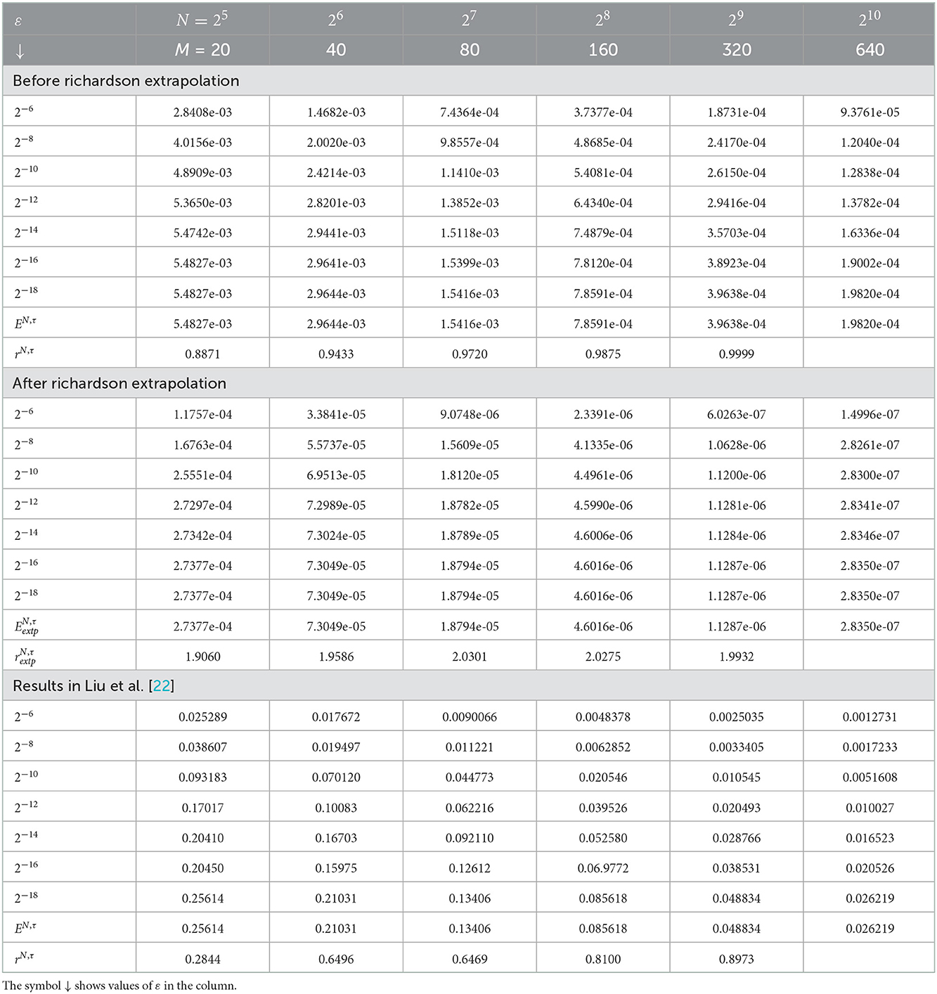
Table 1. Comparison of $E_{\epsilon }^{N,\tau },E^{N,\tau }$, r^{N, τ}, $(E_{\epsilon }^{N,\tau })extp$, $E_{extp}^{N,\tau }$, and $r_{extp}^{N,\tau }$ for Example 5.1 with results in Liu et al. [22].

TABLE 2

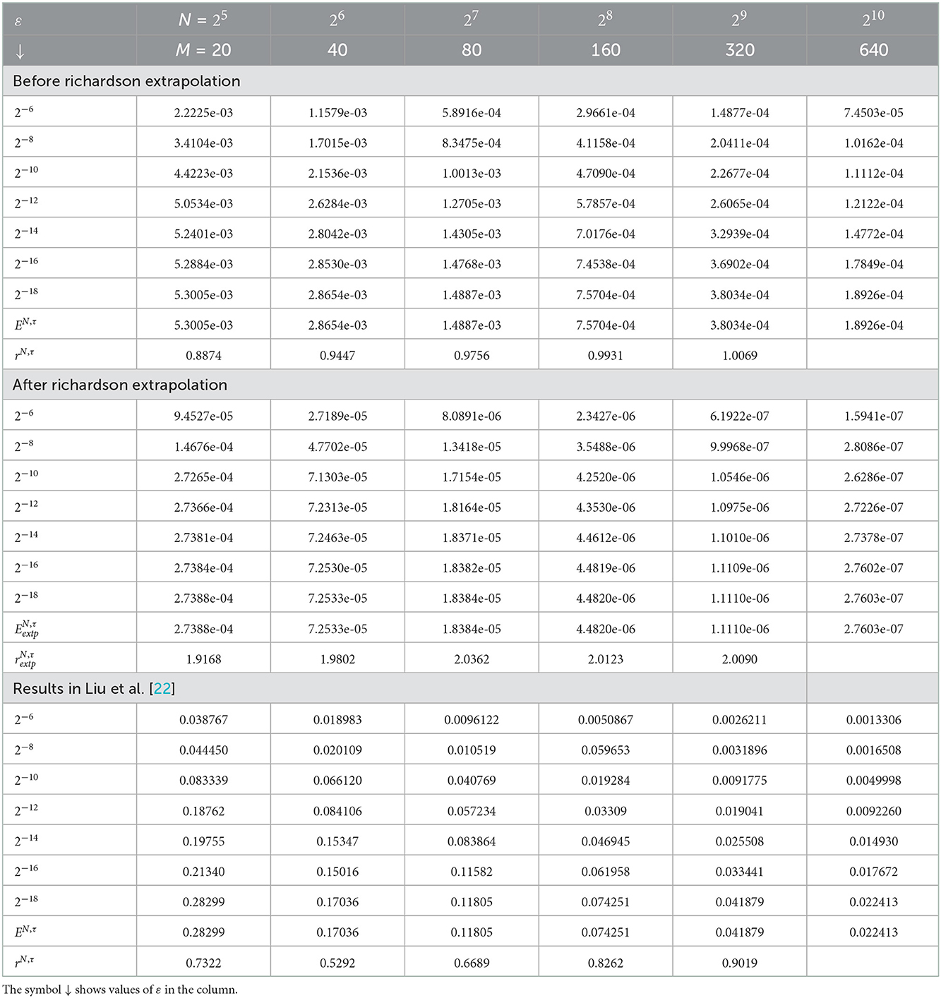
Table 2. Comparison of $E_{\epsilon }^{N,\tau },E^{N,\tau }$, r^{N, τ}, $(E_{\epsilon }^{N,\tau })extp$, $E_{extp}^{N,\tau }$, and $r_{extp}^{N,\tau }$ for Example 5.2 with results in Liu et al. [22].

TABLE 3

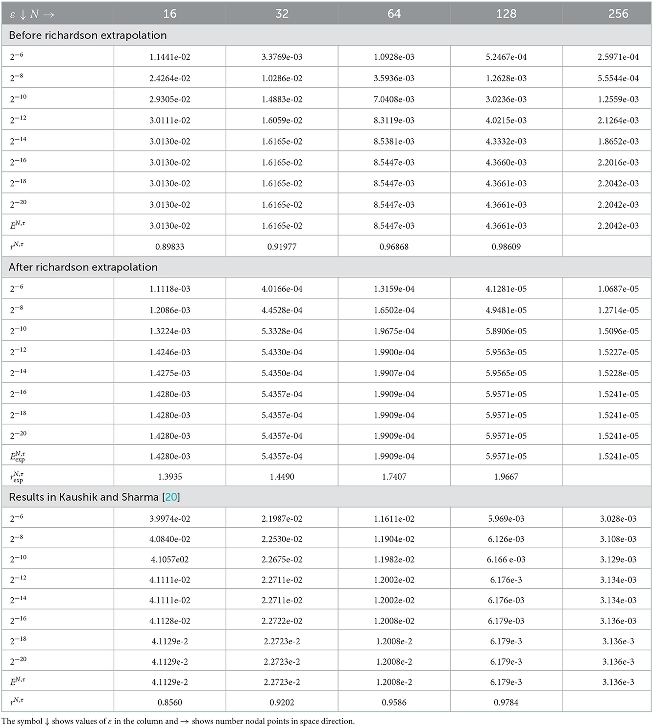
Table 3. Comparison of $E_{\epsilon }^{N,\tau },E^{N,\tau }$, r^{N, τ}, $(E_{\epsilon }^{N,\tau })extp$, $E_{extp}^{N,\tau }$, and $r_{extp}^{N,\tau }$ for Example 5.3 with results in Kaushik and Sharma [20] for τ = 0.001.

TABLE 4

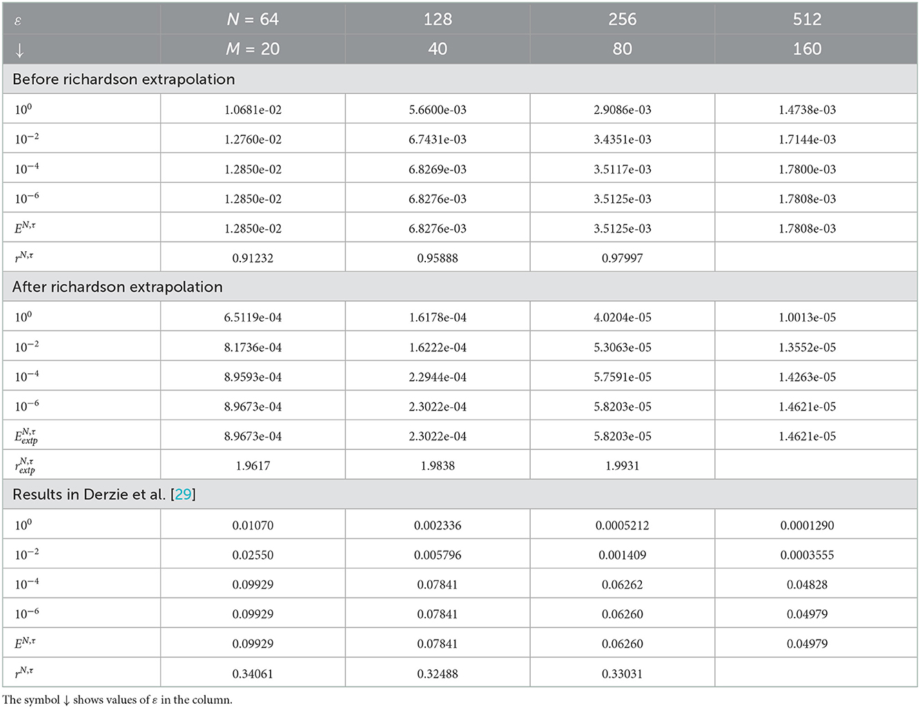
Table 4. Comparison of $E_{\epsilon }^{N,\tau },E^{N,\tau }$, r^{N, τ}, $(E_{\epsilon }^{N,\tau })extp$, $E_{extp}^{N,\tau }$, and $r_{extp}^{N,\tau }$ for Example 5.4 with results in Derzie et al. [29].

FIGURE 1

Figure 1. Numerical solution for N = 64, M = 40, and ε = 2⁻¹⁸ (A) Example 5.1 and (B) Example 5.2.

FIGURE 2

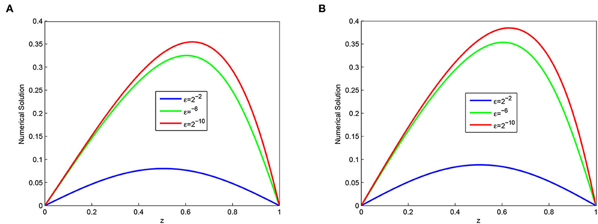
Figure 2. Effect of the ε on behavior of the solution with layer formation (A) Example 5.1 and (B) Example 5.2.

FIGURE 3

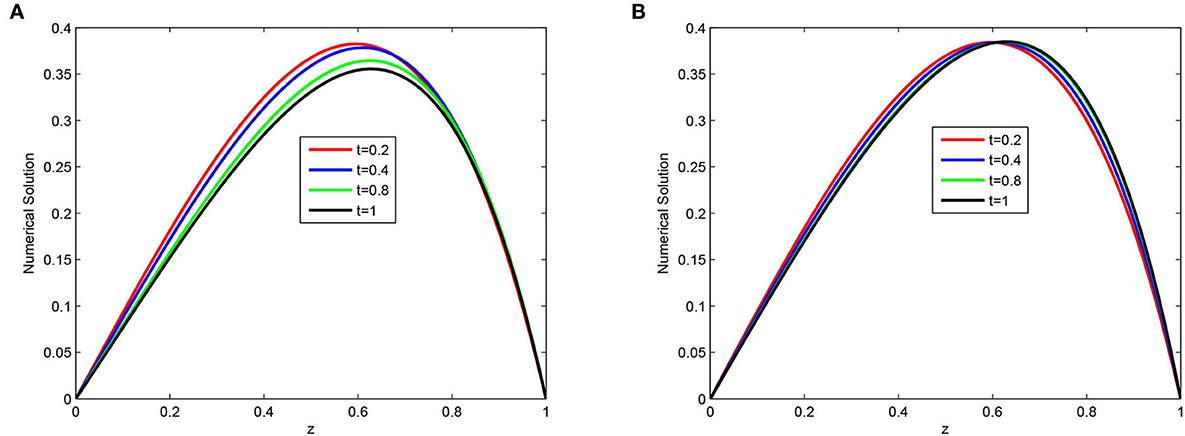
Figure 3. Numerical solution for N = 64, M = 40, and ε = 2⁻¹⁶ and at different time levels (A) Example 5.1 and (B) Example 5.2.

FIGURE 4

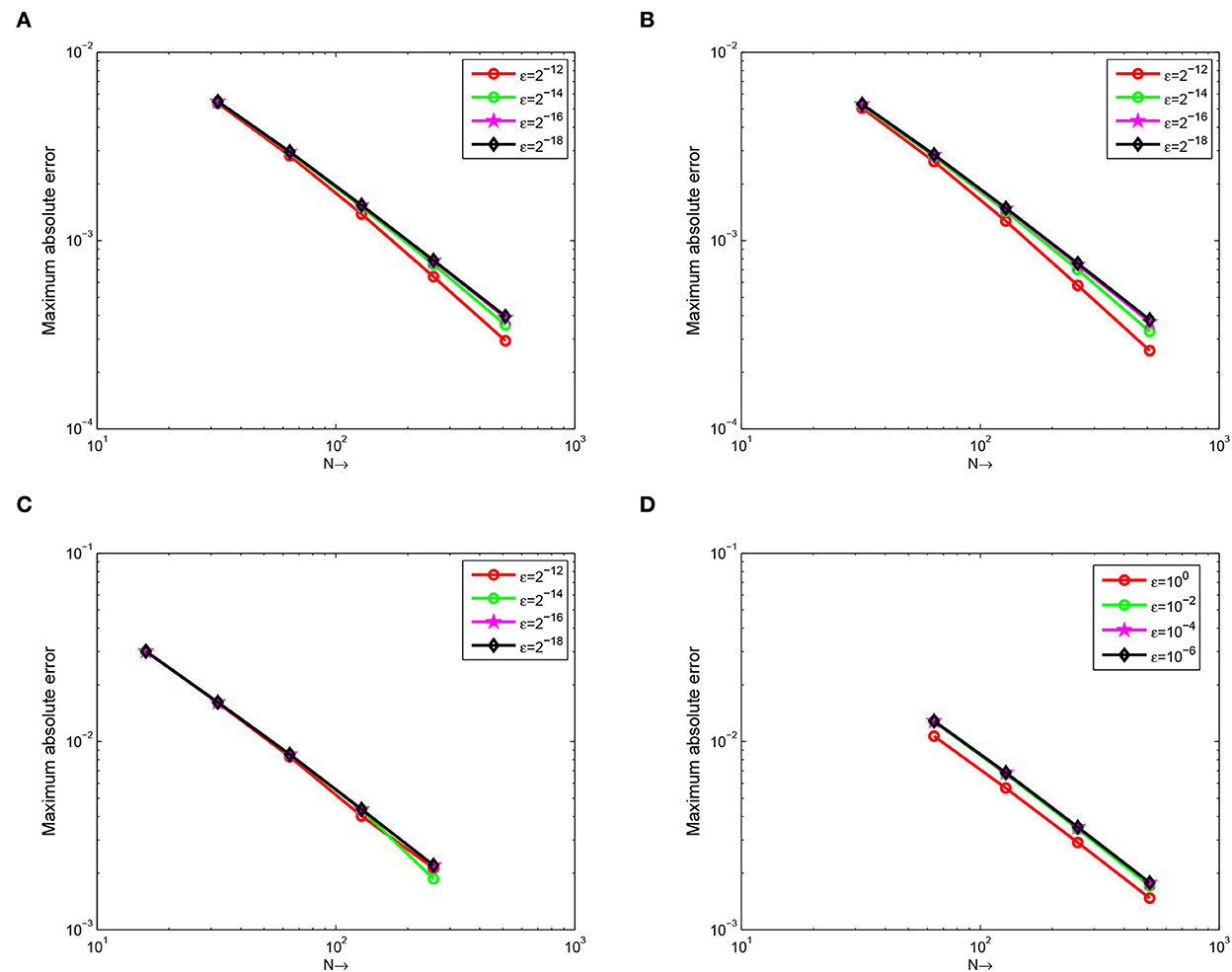
Figure 4. Example 5.1 on (A), Example 5.2 on (B), Example 5.3 on (C), and Example 5.4 on (D), the error plot for different values of ε.

6. Conclusion

A higher order parameter uniform numerical scheme for singularly perturbed unsteady Burger-Huxley equation is presented. The developed scheme constitutes the implicit Euler in the time variable and the exponential spline method in the space variable. In addition, Richardson's extrapolation technique is implemented to improve the accuracy in the time direction. The stability and convergence analysis of the scheme are discussed and proved. It is found that the scheme proposed is uniformly convergent with linear and second order convergent before and after Richardson extrapolation. Four test examples are presented to illustrate the efficiency of the proposed scheme. It is found that the proposed scheme gives better results than the methods described in Derzie et al. [29], Kaushik and Sharma [20], and Liu et al. [22].

Data availability statement

The original contributions presented in the study are included in the article/supplementary material, further inquiries can be directed to the corresponding author.

Author contributions

ITD and GFD: conceptualization, investigation and formal analysis, and visualization. ITD: software programming and writing—original draft. GFD: writing—review and editing. All authors contributed to the article and approved the submitted version.

Acknowledgments

The authors would like to thank the editor and referees for careful reading and giving prolific comments.

Conflict of interest

The authors declare that the research was conducted in the absence of any commercial or financial relationships that could be construed as a potential conflict of interest.

Publisher's note

All claims expressed in this article are solely those of the authors and do not necessarily represent those of their affiliated organizations, or those of the publisher, the editors and the reviewers. Any product that may be evaluated in this article, or claim that may be made by its manufacturer, is not guaranteed or endorsed by the publisher.

References

1. Duan L, Lu Q. Bursting oscillations near codimension-two bifurcations in the chay neuron model. Int J Nonlinear Sci Numer Simulat. (2006) 7:59–64. doi: 10.1515/IJNSNS.2006.7.1.59

CrossRef Full Text | Google Scholar

2. Liu S, Fan T, Lu Q. The spike order of the winnerless competition (wlc) model and its application to the inhibition neural system. Int J Nonlinear Sci Num Simulat. (2005) 6:133–38. doi: 10.1515/IJNSNS.2005.6.2.133

CrossRef Full Text | Google Scholar

3. Aronson DG, Weinberger HF. Multidimensional nonlinear diffusion arising in population genetics. Adv Math. (1978) 30:33–76. doi: 10.1016/0001-8708(78)90130-5

CrossRef Full Text | Google Scholar

4. Zhang, G.-J., Xu, J.-X., Yao H, Wei, R.-X. Mechanism of bifurcation-dependent coherence resonance of an excitable neuron model. Int J Nonlinear Sci Num Simulat. (2006) 7:447–50. doi: 10.1515/IJNSNS.2006.7.4.447

CrossRef Full Text | Google Scholar

5. Lewis E, Reiss R, Hamilton H, Harmon L, Hoyle G, Kennedy D. An electronic model of the neuron based on the dynamics of potassium and sodium ion fluxes. Neural Theory and Modeling. Stanford University Press (1964). pp. 154–89.

6. Ismail HN, Raslan K, Abd Rabboh AA. Adomian decomposition method for burger's-huxley and burger's-fisher equations. Appl Math Comput. (2004) 159:291–301. doi: 10.1016/j.amc.2003.10.050

CrossRef Full Text | Google Scholar

7. Javidi M, Golbabai A. A new domain decomposition algorithm for generalized burger's-huxley equation based on chebyshev polynomials and preconditioning. Chaos Solitons Fractals. (2009) 39:849–57. doi: 10.1016/j.chaos.2007.01.099

CrossRef Full Text | Google Scholar

8. Estevez P. Non-classical symmetries and the singular manifold method: the burgers and the burgers-huxley equations. J Phys A Math Gen. (1994) 27:2113. doi: 10.1088/0305-4470/27/6/033

CrossRef Full Text | Google Scholar

9. Krisnangkura M, Chinviriyasit S, Chinviriyasit W. Analytic study of the generalized burger's-huxley equation by hyperbolic tangent method. Appl Math Comput. (2012) 218:10843–7. doi: 10.1016/j.amc.2012.04.044

CrossRef Full Text | Google Scholar

10. Satsuma J, Ablowitz M, Fuchssteiner B, Kruskal M. Topics in soliton theory and exactly solvable nonlinear equations. Phys Rev Lett. (1987). doi: 10.1142/9789814542210

CrossRef Full Text | Google Scholar

11. Wang X, Zhu Z, Lu Y. Solitary wave solutions of the generalised burgers-huxley equation. J Phys A Math Gen. (1990) 23:271. doi: 10.1088/0305-4470/23/3/011

CrossRef Full Text | Google Scholar

12. Hashim I, Noorani MSM, Al-Hadidi MS. Solving the generalized burgers-huxley equation using the adomian decomposition method. Math Comput Model. (2006) 43:1404–11. doi: 10.1016/j.mcm.2005.08.017

CrossRef Full Text | Google Scholar

13. Hashim I, Noorani M, Batiha B. A note on the adomian decomposition method for the generalized huxley equation. Appl Math Comput. (2006) 181:1439–45. doi: 10.1016/j.amc.2006.03.011

CrossRef Full Text | Google Scholar

14. Khattak AJ. A computational meshless method for the generalized burger's-huxley equation. Appl Math Model. (2009) 33:3718–29. doi: 10.1016/j.apm.2008.12.010

CrossRef Full Text | Google Scholar

15. Mohammadi R. B-spline collocation algorithm for numerical solution of the generalized burger's-huxley equation. Num Methods Partial Differ Equ. (2013) 29:1173–91. doi: 10.1002/num.21750

CrossRef Full Text | Google Scholar

16. Sari M, Gürarslan G. Numerical solutions of the generalized burgers-huxley equation by a differential quadrature method. Math Probl Eng. (2009) 2009:765. doi: 10.1155/2009/370765

CrossRef Full Text | Google Scholar

17. Appadu AR, Inan B, Tijani YO. Comparative study of some numerical methods for the Burgers-Huxley equation. Symmetry. (2019) 11:1333. doi: 10.3390/sym11111333

CrossRef Full Text | Google Scholar

18. Appadu AR, Tijani YO, Aderogba AA. On the performance of some NSFD methods for a 2-D generalized Burgers-Huxley equation. J Diff Equ Appl. (2021) 27:1537–73. doi: 10.1080/10236198.2021.1999433

CrossRef Full Text | Google Scholar

19. Appadu AR, Tijani YO. 1D Generalised burgers-huxley: proposed solutions revisited and numerical solution using FTCS and NSFD methods. Front Appl Math Stat. (2022) 1:773733. doi: 10.3389/fams.2021.773733

CrossRef Full Text | Google Scholar

20. Kaushik A, Sharma M. A uniformly convergent numerical method on non-uniform mesh for singularly perturbed unsteady burger-huxley equation. Appl Math Comput. (2008) 195:688–706. doi: 10.1016/j.amc.2007.05.067

PubMed Abstract | CrossRef Full Text | Google Scholar

21. Gupta V, Kadalbajoo MK. A singular perturbation approach to solve burgers-huxley equation via monotone finite difference scheme on layer-adaptive mesh. Commun Nonlinear Sci Num Simulat. (2011) 16:1825–44. doi: 10.1016/j.cnsns.2010.07.020

CrossRef Full Text | Google Scholar

22. Liu L-B, Liang Y, Zhang J, Bao X. A robust adaptive grid method for singularly perturbed burger-huxley equations. Electron Res Arch. (2020) 28:1439. doi: 10.3934/era.2020076

CrossRef Full Text

23. Kabeto MJ, Duressa GF. Accelerated nonstandard finite difference method for singularly perturbed burger-huxley equations. BMC Res Notes. (2021) 14:1–7. doi: 10.1186/s13104-021-05858-4

PubMed Abstract | CrossRef Full Text | Google Scholar

24. Jima KM, File DG. Implicit finite difference scheme for singularly perturbed burger-huxley equations. J Partial Diff Equat. (2022) 35:87–100. doi: 10.4208/jpde.v35.n1.6

CrossRef Full Text | Google Scholar

25. Kehinde OO, Munyakazi JB, Appadu AR. A NSFD discretization of two-dimensional singularly perturbed semilinear convection-diffusion problems. Front Media. (2022) 8:861276. doi: 10.3389/fams.2022.861276

CrossRef Full Text | Google Scholar

26. Zahra WK, Ashraf MEM. Numerical solution of two-parameter singularly perturbed boundary value problems via exponential spline. J King Saud Univer Sci. (2013) 25:201–8. doi: 10.1016/j.jksus.2013.01.003

CrossRef Full Text | Google Scholar

27. O'Malley JRE. Introduction to singular perturbations. Technical report, New York Univ Ny Courant Inst of Mathematical Sciences (1974).

28. Nichols N. On the numerical integration of a class of singular perturbation problems. J Optim Theory Appl. (1989) 60:2050034. doi: 10.1007/BF00940347

CrossRef Full Text | Google Scholar

29. Derzie EB, Munyakazi JB, Gemechu T. A parameter-uniform numericalmethod for singularly perturbed burgers' equation. Comput Appl Math. (2022) 41:1–19. doi: 10.1007/s40314-022-01960-w

CrossRef Full Text | Google Scholar

30. Venkata RKAS, Palli MMK. A numerical approach for solving singularly perturbed convection delay problems via exponentially fitted spline method. Calcolo. (2017) 54:943–61. doi: 10.1007/s10092-017-0215-6

CrossRef Full Text | Google Scholar

31. Gupta V, Kadalbajoo MK, Dubey RK. A parameter-uniform higher order finite difference scheme for singularly perturbed time-dependent parabolic problem with two small parameters. Int J Comput Math. (2019) 96:474–99. doi: 10.1080/00207160.2018.1432856

CrossRef Full Text | Google Scholar