Reduction of uncertainty using adaptive modeling under stochastic criteria of information content

1. Introduction

The importance of a chosen criterion in creating a sound statistical choice cannot be overstated [1]. The undefined behavior of random parameters is the most challenging to investigate however, an appropriately established criterion, the ambiguity produced ought to be minimized [2]. The “Entropy” concept is extensively used in the mathematics and recently started to use in social sciences. Therefore, entropy concept is used for the building models in the planning process [3]. Entropy can be used to gauge the degree of disorder in a given system, resulting in a measurement of the degree of data uncertainty [4]. The strategy's entropy, or level of uncertainty, can be reduced by information collection [5]. The less unknown the system's condition is, the more knowledge there is about entropy and information are frequently used as indicators of uncertainty in probability distributions [6].

Despite being expressed in a complex mathematical language, the idea of probability represents the characteristics of probability that are frequently seen in daily life. For instance, each set of spots produced by the simple die toss corresponds to an actual random event whose probability is represented by the positive real number. When a simple die is thrown, the probability of two (or more) digits of spots is equal to the product of their probabilities (relation). All conceivable numbers of spots' cumulative probability are normed to one link.

The theory of probability and mathematical statistics serve as the mathematical foundation for both applied statistics and statistical analytic techniques. Entropy is a measure of uncertainty and probability distribution in mathematics statistics. Information theory is quantitatively defined in mathematics and is sometimes referred to as informational or statistical entropy. Statistical and informational science has long debated the functional link between entropy and the corresponding probability distribution.

Numerous connections have been made based on the characteristics of entropy. Characteristics, such as additivity, extensivity in the Shannon information theory, are posited in the conventional information theory and some of its extensions. It is often referred to as Shannon's entropy in mathematics. Here, we took a mathematical statistics approach to the widely studied decision subject. Our framework's starting point is a normative definition of uncertainty that connects a physical system's uncertainty measure to evidence via a probability distribution. The paper is structured as follows: Section 2 analyses various existing methods reviews employed so far. Section 3 is a detailed explanation of the proposed methodology. The performance analysis of the proposed method is estimated, and the outcomes are projected in Section 4. At last, the conclusion of the work is made in Section 5.

2. Shannon informational entropy

The following list includes several entropies that have been proposed based on supported entropy features. The most well-known of these entropies is the Shannon informational entropy, or Boltzmann-Gibbs entropy (S = $-\sum _i{p}_{i}ln{p}_i$) [7]. which is virtually and usually engaged in non-equilibrium dynamics and equilibrium thermodynamics. The scientific community is divided about whether Shannon entropy is a unique and valuable indicator of statistical uncertainty or information [8]. The maximum entropy density is obtained by maximizing Shannon's [9] entropy measure.

Jaynes's maximization of entropy (maxent) principle asserted that the Shannon entropy is the only reliable indicator of uncertainty maximized in maxent [10]. One naturally wonders what would happen if some of these features changed because of this particular information property from the Shannon postulates [11].

Some of the entropies are discovered via mathematical reasoning that modifies Shannon's logic [12]. Non-extensive statistics (NES) were recently proposed using some entropy for stochastic dynamics and thermodynamics of particular non-extensive systems [13, 14]. NES has sparked a lot of publications with very different perspectives on equilibrium and non-equilibrium systems, leading to a lot of discussion [15] among statistical physicists. In the discussion, some critical issues include whether Boltzmann Gibbs-Shannon entropy should be swapped out for another in a different physical scenario. What may be maximized to have the maximum probability distribution?

The entropy forms used in maxent applications must be either explicitly posited or derived from the entropy's claimed properties [16]. The reliability of the calculated probability distributions serves as evidence for the soundness of these entropies. Ahmad et al. [17], the amount of information is measured by decreasing the entropy of such a system. The amount of information acquired in the complete clarification of the state of a certain physical system is equal to the entropy of this system as shown in Equation (1)

$\begin{array}{ll}{I}_X=H(X)-0=H(X).& (1)\end{array}$

The average (or complete) information obtained from all possible individual observations can be rewritten in the form of the mathematical expectation of the logarithm of the state probability with the opposite sign

$\begin{array}{ll}{I}_X=M\left[-lnP(X)\right].& (2)\end{array}$

For continuous random variables, expression (2) is written in the form

$\begin{array}{ll}{I}_X=-{\displaystyle {\int }_{-\infty }^{\infty }}f(x)ln\left[f(x)\right]dx,& (3)\end{array}$

where, f(x) – distribution density of a random variable x.

Therefore, it is necessary that the statistics of the criterion ensures the receipt of the maximum amount of information from the available statistical material about the system. Let us consider the limiting case when information about the system is represented by a sample of independent random variables X₁and X₂ of minimal volume n = 2. In the absence of other data, the principle of maximum uncertainty postulates the use of a uniform distribution on the interval [a; b] [18] where, a = min{X₁, X₂} and b = max{X₁, X₂}. For definiteness, let us consider a = 0 and b = 1.

To compare two independent random variables X₁ and X₂, evenly distributed in the interval [0; 1], we use two main metrics ${\delta }_1=\frac{X_1}{X_2}$ and δ₂ = X₂ − X₁, X₁ ≤ X₂. Note that besides δ₁ and δ₂ other metrics are possible, which, in essence, are functions δ₁ and δ₂. However, for any transformation of the original random variable δ the loss of information is inevitable; the total conditional entropy of the system does not exceed its unconditional entropy [19]

$\begin{array}{ll}H(\delta |X)\le H(\delta ),X=X(\delta ).& (4)\end{array}$

To compare the information content of metrics δ₁ and δ₂ [their entropies (3)] it is necessary to determine the distribution density of f(δ₁) and g(δ₂). The density of the joint distribution of ordered random variables, uniformly distributed in the interval [0; 1], will be written in the form [3]

$\begin{array}{ll}f(x,y)=2!f_x(x)f_y(y)=2& (5)\end{array}$

where, f_x(x) = 1 and f_y(y) = 1 – distribution density of independent random variables x and y.

Let us consider transformation variables

$\begin{array}{l}{y}_1=\frac{x_1}{x_2},y_2=x_2.\end{array}$

or

$\begin{array}{l}{x}_1=y_1{x}_2=y_1{y}_{2}and{x}_2=y_2.\end{array}$

The Jacobian of the transformation has the form [20]

$\begin{array}{l}J=\frac{\partial (x_1,x_2)}{\partial (y_1,y_2)}=\left|\begin{array}{c}{y}_{2}0\\ y_{1}1\end{array}\right|=y_2.\end{array}$

Then the joint distribution density [21]

$\begin{array}{l}g(y_1,y_2)=f(x_1,x_2)J|\begin{array}{c}{x}_1=y_1{y}_2\\ x_2=y_2\end{array}=2y_2.\end{array}$

where,

$\begin{array}{l}g(y_1)={\displaystyle {\int }_0^1}g(y_1,y_2)d{y}_2={\displaystyle {\int }_0^1}2y_{2}d{y}_2=2\frac{y_2^2}{2}|\begin{array}{c}1\\ 0\end{array}=1.\end{array}$

That is, the metric δ₁ obeys the uniform distribution law on the interval [0; 1]. Figure 1 shows a histogram of the metric distribution δ₁.

FIGURE 1

Figure 1. Checking for the uniformity of the metric distribution δ₁.

It can be seen that when the hypothesis of a uniform distribution is rejected, an error is made with probability (attainable level of significance) p = 0.67. Therefore, the reasons to reject the hypothesis that the metric is uniformly distributed with density

$\begin{array}{ll}f({\delta }_1)=1& (6)\end{array}$

are absent.

Difference density δ₂ = X₂ − X₁ of random variables X₁ ≤ X₂ [1].

$\begin{array}{l}g({\delta }_2)={\displaystyle {\int }_{-\infty }^{\infty }}f(x_2-{\delta }_2,x_1)d{x}_1={\displaystyle {\int }_0^{1-{\delta }_2}}2d{x}_1\end{array}$

$\begin{array}{ll}=2x_1|\begin{array}{c}1-{\delta }_2\\ 0\end{array}=2(1-{\delta }_2).& (7)\end{array}$

Figure 2 shows the result of checking the uniformity of a random variable υ = G(δ₂), where G(δ₂) – metric distribution function δ₂.

FIGURE 2

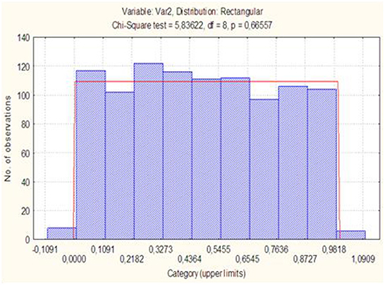
Figure 2. Checking for the uniformity of a random variable υ = G(δ₂).

As the p-level is p = 0.15, then we can say that the results of the experiment indicate an error when rejecting the hypothesis of a uniform distribution of the random variable υ = G(δ₂) with probability of 0.15. This is more than a level of significance α = 0.1. Therefore, the sufficient grounds for rejecting the hypothesis of the uniform distribution of the random variable υ = G(δ₂) aren't present.

Thus, density (7) describes the law of distribution of the modulus of the difference of independent random variables uniformly distributed over the interval [0; 1].

Figure 3 shows a histogram of the metric distribution δ₂, from the nature of the density of which it can be seen that it belongs to the class of beta distributions [22]

$\begin{array}{l}g({\delta }_2)={{\delta }_2}^{a-1}{(1-{\delta }_2)}^{b-1},{\delta }_2\in \left[0;1\right]\end{array}$

with parameters a = 1 and b = 2, after substitution of which we obtain expression (7). Thus, in one interval [0; 1] we have distributions of two random metrics with different laws.

FIGURE 3

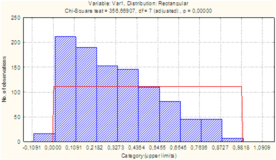
Figure 3. Histogram of the metric distribution δ₂.

It was shown above that the informativeness of the criteria is determined by the Shannon entropy (3), which for these metrics will take the following values:

$\begin{array}{l}{H}_{{\delta }_1}=-{\displaystyle {\int }_0^1}f({\delta }_1)ln\left[f({\delta }_1)\right]d{\delta }_1=-{\displaystyle {\int }_0^1}ln1d{\delta }_1=0.\\ H_{{\delta }_2}=-{\displaystyle {\int }_0^1}g({\delta }_2)ln\left[g({\delta }_2)\right]d{\delta }_2=0.5-ln2=-0.19.\end{array}$

It is not hard to see that H_δ1 > H_δ2, meaning that according to entropy the metric δ₁ dominates the metric δ₂.

The ratio of two independent ordered random variables, uniformly distributed on the interval [0; 1], is more informative than their difference. In practice, this conclusion means that to construct a criterion based on a sample of independent random variables uniformly distributed in the interval [0; 1], in the absence of any additional conditions, preference should be given to their ratio.

The uniform law can serve as the basis for the criteria for making statistical decisions, while being a very simple distribution to implement and tabulate. Therefore, its identification (testing the hypothesis of a uniform distribution law) is a topical research topic in order to determine the most powerful goodness-of-fit criteria. Much attention has been paid to this issue recently, and the result of a comprehensive analysis was work [23], in which the authors investigated the power of the known criteria for samples of size n ≥ 10.

Samples of a smaller size are considered to be small, the theory of making statistical decisions on which, under the conditions of non-asymptotic formulation of problems, currently still needs to be scientifically substantiated and developed. The complexity of the formulation and solution of the problems of constructing the best estimates for a given volume of statistical material is due to the fact that the desired solution often strongly depends on the specific type of distribution the sample size and cannot be an object of a sufficiently general mathematical theory [24].

3. Methodology

The probabilistic model provides for the summation of independent random variables, then the sum is naturally described by the normal distribution. In our work, we consider the limiting case when information about the system is represented by a sample of minimum size. The principle of maximum entropy stated that typical distributions of probabilities of states of an uncertain situation are those it increases the selected measure of uncertainty for specified information in relation to the “behavior” of the situation. In the absence of other data, the principle of maximum uncertainty postulates the use of a uniform distribution on the interval [a; b]. Since it is customary to use entropy as a measure of the uncertainty of a certain physical system. A stochastic multi-criteria preference model (SMCPM) method integrated with optimization approach will be developed for addressing stochasticity of input information.

3.1. Stochastic similarity criterion

It is possible to construct a criterion of uniformity of random variables (agreement), which is a convolution of particular criteria of uniformity for making a statistical decision on it. Moreover, the generalization of the theorem on the ratio of the smaller of two independent random variables uniformly distributed in the interval [0; 1] to the larger one consists in the formulation and proof of the following theorem.

3.1.1. Theorem

Let a sample of independent random variables be given x₁, x₂, ..., x_n, uniformly distributed in the interval [0; 1] and let them compose the corresponding variation series$x_1^{{}^{\prime }}\le x_2^{{}^{\prime }}\le ...\le x_n^{{}^{\prime }}$. Dividing all the members of this variation series (except for $x_n^{{}^{\prime }}$) by $x_n^{{}^{\prime }}$, we will get υ₁ ≤ υ₂ ≤ ... ≤ υ_k, k = n − 1. Proceeding in the same way with this and subsequent rows, as a result we get a random variable V₁, uniformly distributed in the interval [0; 1].

3.1.2. Evidence

Sample volume case n = 2. A variation series was compiled from the observations of the sample x₁ ≤ x₂ (here and below, to simplify the notation, the terms of the variation series are not marked with a prime). Probability density of joint distribution of ordered random variables x₁ ≤ x₂ will be written as follows [25].

$\begin{array}{ll}{f}_{x_1,x_2}(x_1,x_2)=2!{\displaystyle \prod _{i=1}^2}{f}_{x_i}(x_i)=2!,& (8)\end{array}$

where f_xi(x_i) = 1 – distribution density of i observation in the sample.

Let us introduce into consideration two statistics (by the number of terms of the variational series)

$\begin{array}{ll}{\upsilon }_1=\frac{x_1}{x_2}and{\upsilon }_2=x_2.& (9)\end{array}$

Since the inverse transformations of random variables in Equation (9)

x₁ = υ₁υ₂ and x₂ = υ₂ are one-to-one, then the joint distribution density

$\begin{array}{ll}{f}_{{\upsilon }_1,{\upsilon }_2}({\upsilon }_1,{\upsilon }_2)=f_{x_1,x_2}{(x_1,x_2)}_{x_i=x_i({\upsilon }_1,{\upsilon }_2)}·\left|J\right|,& (10)\end{array}$

where $J=\frac{\partial (x_1,x_2)}{\partial ({\upsilon }_1,{\upsilon }_2)}=\left|\begin{array}{c}{\upsilon }_{2}0\\ {\upsilon }_{1}1\end{array}\right|={\upsilon }_2$ – Jacobian.

Then, taking into account (8), the joint distribution density (10) will be written as follows

$\begin{array}{ll}{f}_{{\upsilon }_1,{\upsilon }_2}({\upsilon }_1,{\upsilon }_2)=2!{\upsilon }_2.& (11)\end{array}$

Excluding the helper variable υ₂ by integrating expression (11) over the range of values of υ₂, we will get the density of the variable υ₁

$\begin{array}{ll}{f}_{{\upsilon }_1}({\upsilon }_1)={\displaystyle {\int }_0^1}{f}_{{\upsilon }_1,{\upsilon }_2}({\upsilon }_1,{\upsilon }_2)d{\upsilon }_2={\displaystyle {\int }_0^1}2{\upsilon }_{2}d{\upsilon }_2=1!& (12)\end{array}$

(the factorial sign is left to summarize the results).

Result (12) testifies to the uniform distribution law of the variable υ₁. Figure 4 shows histograms of distributions of statistics x₁ ≤ x₂, from which it can be assumed that statisticians are subject to the law.

FIGURE 4

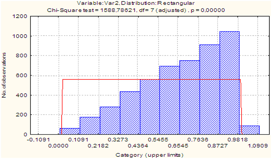
Figure 4. Histograms of distributions of statistics x₁ ≤ x₂ of beta distribution.

The test showed that the achieved significance levels for the corresponding hypotheses with beta distribution parameters α = 1, β = 2 for the statistic of x₁(p = 0.66) and α = 2, β = 1 for the statistic of x₂(p = 0.3) testify against their rejection [10].

Figure 5 shows the histogram and the result of checking the uniformity of statistics υ₁, from which it is clear that the achieved level of significance (p = 0.2) also testifies against the rejection of the hypothesis of its uniform distribution (or beta distribution with parameters α = 1, β = 1).

FIGURE 5

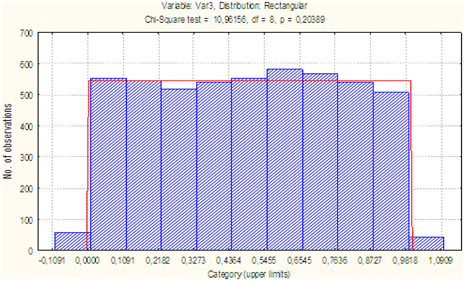
Figure 5. Histogram of statistics distribution υ₁.

Sample volume case n = 3. For it, the variational series has the form x₁ ≤ x₂ ≤ x₃. Let's introduce statistics

$\begin{array}{ll}{\upsilon }_1=\frac{x_1}{x_3},{\upsilon }_2=\frac{x_2}{x_3}and{\upsilon }_3=x_3& (13)\end{array}$

unique inverse transformations for which have the form x₁ = υ₁υ₃, x₂ = υ₂υ₃ and x₃ = υ₃.

Jacobian transformation

$\begin{array}{l}J=\frac{\partial (x_1,x_2,x_3)}{\partial ({\upsilon }_1,{\upsilon }_2,{\upsilon }_3)}=\left|\begin{array}{c}{\upsilon }_{3}00\\ 0{\upsilon }_{3}0\\ {\upsilon }_1{\upsilon }_{2}1\end{array}\right|={\upsilon }_3^2.\end{array}$

The density of the joint distribution of the members of the variation series υ₁ ≤ υ₂ ≤ υ₃ taking into account the sample size for (8) and (10) will take the form $f_{{\upsilon }_1,{\upsilon }_2,{\upsilon }_3}({\upsilon }_1,{\upsilon }_2,{\upsilon }_3)=3!{\upsilon }_3^2$. The density of the joint distribution of statistics of υ₁ ≤ υ₂ is

$\begin{array}{l}{f}_{{\upsilon }_1,{\upsilon }_2}({\upsilon }_1,{\upsilon }_2)={\displaystyle {\int }_0^1}{f}_{{\upsilon }_1,{\upsilon }_2,{\upsilon }_3}({\upsilon }_1,{\upsilon }_2,{\upsilon }_3)d{\upsilon }_3\end{array}$

$\begin{array}{ll}={\displaystyle {\int }_0^1}3!{\upsilon }_3^{2}d{\upsilon }_3=2!.& (14)\end{array}$

For these statistics, two statistics are entered $V_1=\frac{{\upsilon }_1}{{\upsilon }_2}$ and V₂ = υ₂, for which the one-to-one inverse transformations have the form υ₁ = V₁V₂ and υ₂ = V₂.

$\begin{array}{l}\text{Jacobian transformation }J=\frac{\partial ({\upsilon }_1,{\upsilon }_2)}{\partial (V_1,V_2)}=\left|\begin{array}{c}{V}_{2}0\\ V_{1}1\end{array}\right|=V_2.\end{array}$

The density of the joint distribution of the members of the variation series V₁ ≤ V₂ has the form f(V₁, V₂) = 2!V₂. Whence, by integrating with respect to the variable V₂ we will get the distribution density of statistics V₁

$\begin{array}{ll}f(V_1)={\displaystyle {\int }_0^1}f(V_1,V_2)d{V}_2=2{\displaystyle {\int }_0^1}{V}_{2}d{V}_2=1& (15)\end{array}$

which testifies a uniform distribution of statistics V₁in the interval [0; 1].

It can be shown that the distributions of statistics υ₁, υ₂ and their relationship $V_1=\frac{{\upsilon }_1}{{\upsilon }_2}$ also obey the law of beta distribution with attainable levels of significance p_υ1 = 0.03, p_υ2 = 0.33, and p_V1 = 0.75 according to parameters α = 1, β = 2; α = 2, β = 1 and α = 1, β = 1.

It means that statistic V₁ is uniformly distributed in the interval [0; 1]. In accordance with the method of mathematical induction, let us consider sample volume n − 1. The variation series for it is x₁ ≤ x₂ ≤ ... ≤ x_{n− 1}.

Let's introduce the statistic

${\upsilon }_1=\frac{x_1}{x_{n-1}},{\upsilon }_2=\frac{x_2}{x_{n-1}},$ … υ_n−1 = x_n−1, for which the one-to-one inverse transformations have the form

x₁ = υ₁υ_n−1, x₂ = υ₂υ_n−1, …, x_n−1 = υ_{n− 1}.

Jacobian transformation

$\begin{array}{l}J=\frac{\partial (x_1,x_2,...,x_{n-1})}{\partial ({\upsilon }_1,{\upsilon }_2,...{\upsilon }_{n-1})}=\left|\begin{array}{c}{\upsilon }_{n-1}0...0\\ 0{\upsilon }_{n-1}...0\\ ............\\ {\upsilon }_1{\upsilon }_2...1\end{array}\right|={\upsilon }_{n-1}^{n-2}.\end{array}$

The density of the joint distribution of the members of the variation series υ₁ ≤ υ₂ ≤ ... ≤ υ_n−1 taking into account the sample size for (8) and (10) will take the form $f_{{\upsilon }_1,{\upsilon }_2,...,{\upsilon }_{n-1}}({\upsilon }_1,{\upsilon }_2,...,{\upsilon }_{n-1})=(n-1)!{\upsilon }_{n-1}^{n-2}$. Where from the density of the joint distribution of statistics υ₁ ≤ υ₂ ≤ ... ≤ υ_{n− 2}

$\begin{array}{l}{f}_{{\upsilon }_1,{\upsilon }_2,...,{\upsilon }_{n-2}}({\upsilon }_1,{\upsilon }_2,...,{\upsilon }_{n-2})={\displaystyle {\int }_0^1}{f}_{{\upsilon }_1,{\upsilon }_2,...,{\upsilon }_{n-1}}\\ ({\upsilon }_1,{\upsilon }_2,...,{\upsilon }_{n-1})d{\upsilon }_{n-1}\end{array}$

$\begin{array}{ll}=(n-1)!{\displaystyle {\int }_0^1}{\upsilon }_{n-1}^{n-2}d{\upsilon }_{n-1}=(n-2)!.& (16)\end{array}$

The density of the joint distribution of the members of the variation series υ₁ ≤ υ₂ ≤ ... ≤ υ_n−2 taking into account the sample size for (8) and (10) will take the form

$\begin{array}{ll}{f}_{V_1,V_2,...,V_{n-2}}(V_1,V_2,...,V_{n-2})=(n-2)!V_{n-2}^{n-3}& (17)\end{array}$

Whence the density of the joint distribution of the members of the variation series V₁ ≤ V₂ ≤ ... ≤ V_n−3 after integration (17) according to V_{n− 2}

$\begin{array}{l}{f}_{V_1,V_2,...,V_{n-3}}(V_1,V_2,...,V_{n-3})=(n-1)!\end{array}$

Carrying out similar transformations for all statistics V, we will obtain the density of the final one

$\begin{array}{ll}{f}_{V_1}(V_1)=1,& (18)\end{array}$

which indicates a uniform distribution in the interval [0; 1] of the convolution υ_k – criteria (VIC criteria) for a sample size n− 1.

For sample volume n with variation series x₁ ≤ x₂ ≤ ... ≤ x_n let's introduce statistics ${\upsilon }_2=\frac{x_2}{x_n},$ … υ_n = x_n, for which the one-to-one inverse transformations have the form

$\begin{array}{l}{x}_1={\upsilon }_1{\upsilon }_n,x_2={\upsilon }_2{\upsilon }_n,\dots ,x_n={\upsilon }_n.\end{array}$

Jacobian transformation

$\begin{array}{l}J=\frac{\partial (x_1,x_2,...,x_n)}{\partial ({\upsilon }_1,{\upsilon }_2,...{\upsilon }_n)}=\left|\begin{array}{c}{\upsilon }_{n}0...0\\ 0{\upsilon }_n...0\\ ............\\ {\upsilon }_1{\upsilon }_2...1\end{array}\right|={\upsilon }_n^{n-1}.\end{array}$

The density of the joint distribution of the members of the variation series υ₁ ≤ υ₂ ≤ ... ≤ υ_n taking into account the sample size for (8) and (10) will take the form

$\begin{array}{l}{f}_{{\upsilon }_1,{\upsilon }_2,...,{\upsilon }_n}({\upsilon }_1,{\upsilon }_2,...,{\upsilon }_n)=(n)!{\upsilon }_n^{n-1}.\end{array}$

Where from the density of the joint distribution of statistics υ₁ ≤ υ₂ ≤ ... ≤ υ_n−1 is

$\begin{array}{l}{f}_{{\upsilon }_1,{\upsilon }_2,...,{\upsilon }_{n-1}}({\upsilon }_1,{\upsilon }_2,...,{\upsilon }_{n-1})={\displaystyle {\int }_0^1}{f}_{{\upsilon }_1,{\upsilon }_2,...,{\upsilon }_n}({\upsilon }_1,{\upsilon }_2,...,{\upsilon }_n)d{\upsilon }_n\end{array}$

$\begin{array}{ll}=(n)!{\displaystyle {\int }_0^1}{\upsilon }_n^{n-1}d{\upsilon }_n=(n-1)!.& (19)\end{array}$

Further, by analogy with the sample volume n − 1 we introduce statistics V, applying the same procedures for which, it can be shown that the density of the finite of them

$\begin{array}{ll}{f}_{V_1}(V_1)=1,& (20)\end{array}$

This testifies to the uniform distribution in the interval [0; 1] of the convolution of the VIC criteria and for the sample size n.

For illustration, Figure 6 shows histograms of statistic-stick distributions υ₁ ≤ υ₂ for sample volume n = 7.

FIGURE 6

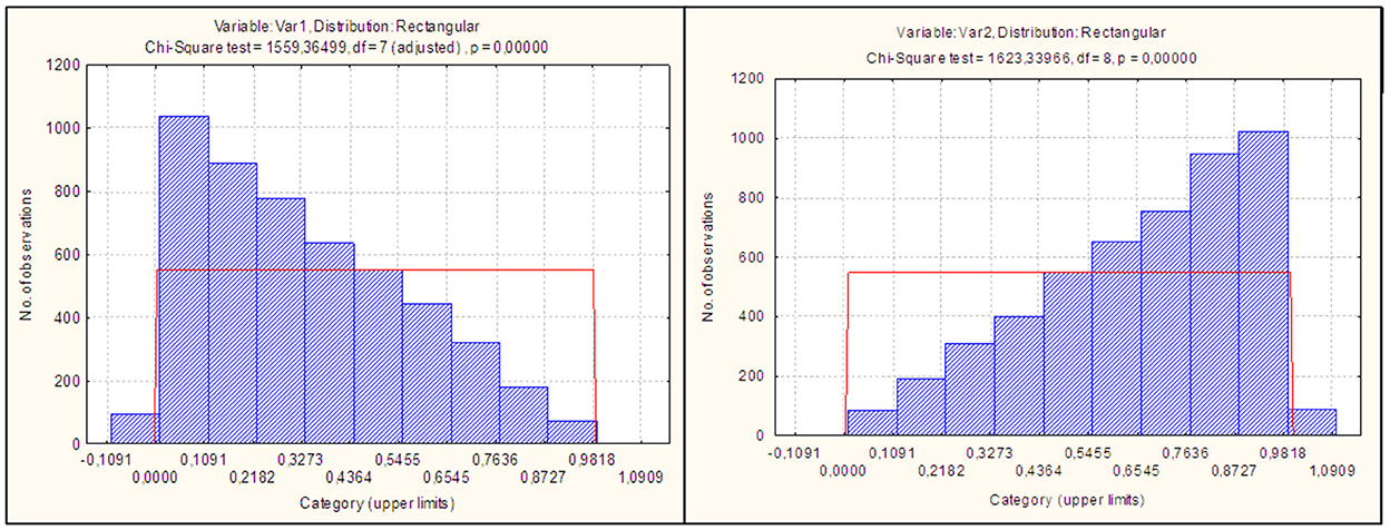
Figure 6. Histograms of distributions of statistics υ₁ ≤ υ₂.

It can see the complete identity of the distribution of statistics x₁ ≤ x₂ (see Figure 4). Also identical to the distribution υ₁ Figure 5 shows the distribution of statistics V₁, whose histogram is shown in Figure 7.

FIGURE 7

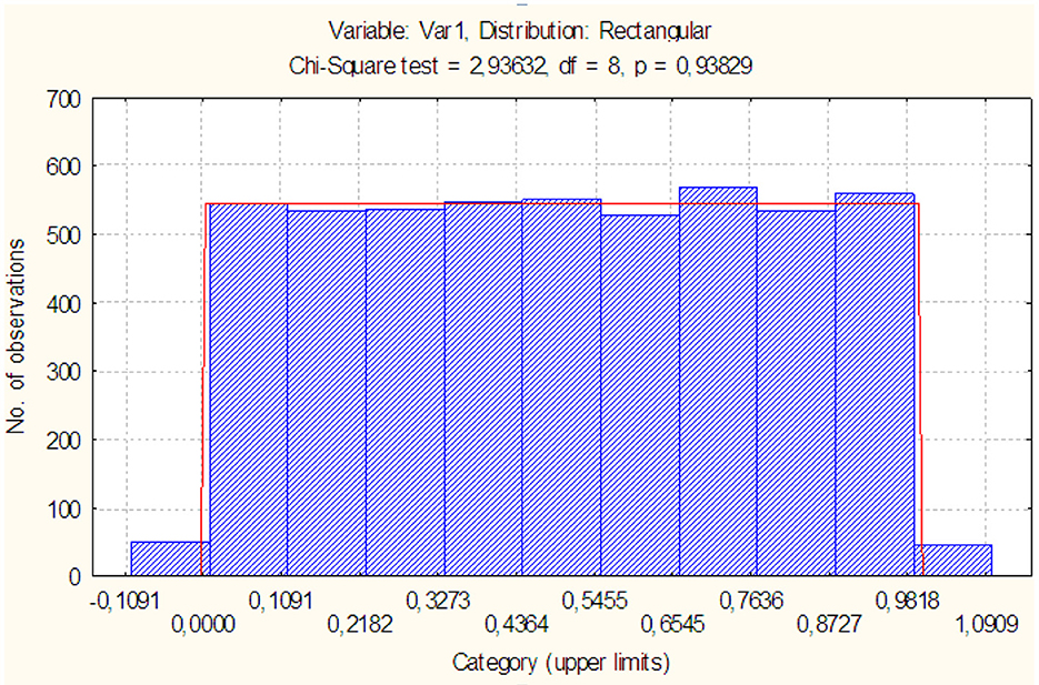
Figure 7. Histogram of statistics distribution V₁.

The figure shows that the achieved level of significance p = 0.94 testifies against the rejection of the hypothesis of its uniform distribution. Thus, the theorem has been proven theoretically and empirically. The achieved level of significance, the decision-making procedure is more flexible: the less is p(s) we see, the stronger the set of observations testifies against the hypothesis being tested [16]. On the other hand, the smaller the value s, the more likely it is that the hypothesis being tested H is true [24].

For their simultaneous accounting, it is proposed to introduce into consideration the relative-level

$\begin{array}{ll}{p}_H=\frac{p(s)}{s}|W.& (21)\end{array}$

Then, when testing the hypothesis H₀ with the alternative H₁ the effectiveness of their differentiation can be judged by the value

$\begin{array}{ll}W=\frac{p_{H_0}-p_{H_1}}{p_{H_0}}.& (22)\end{array}$

4. Result and discussion

Figure 8 shows the results of testing for the uniformity of the hypothesis $H_0:F(x)=x,\begin{array}{c}0x\in \left[0;1\right]\end{array}$ and alternatives to the uniform law in the form of a hypothesis H₁ : F(x) = B_I(1.5, 1.5, 1, 0) about the beta distribution of the first kind.

FIGURE 8

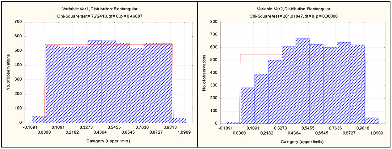
Figure 8. Checking the uniformity of the sample volume n = 2.

Similar results for samples up to without figures are summarized in Table 1.

TABLE 1

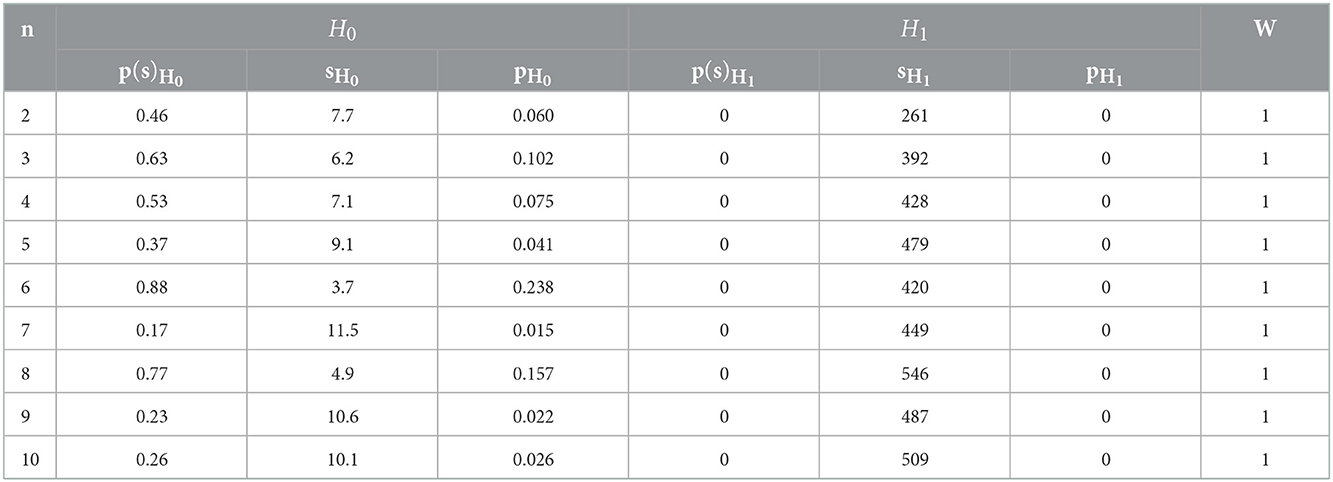
Table 1. Achieved p-levels of the hypothesis H₀ relatively to H₁.

The table shows that the proposed criterion has a high efficiency of distinguishing between hypotheses. H₀ И H₁ in the specified range n. In the traditional assessment of the power of the goodness-of-fit test, Table 2 shows its values for the right-sided critical region and for a sample of n ≤ 10 with the number of realizations 5,000 for each volume.

TABLE 2

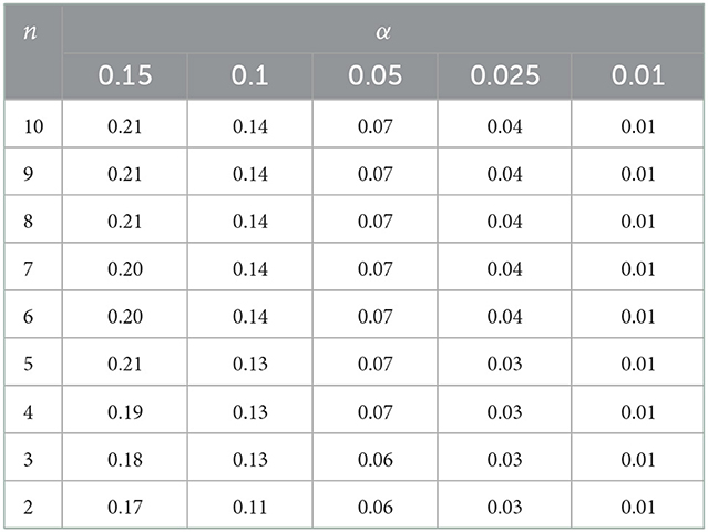
Table 2. Convolution power of the VIC test relative to the hypothesisH₁.

It can be seen from the table that the cardinality of the convolution of the VIC test is higher than the cardinality of the test Z_A Zhang at n = 10, which is at the top of preference among the criteria. Even with minimal sample sizes, it is higher than that of the criterion Z_A Zhang at n = 10, which gives a tangible advantage in distinguishing between such close hypotheses. Thus, the uniformity check procedure, which is simple to implement, can serve as a worthy tool in the study of small-volume samples.

Sample volume n > 10 should be broken down into k = 5...7 intervals as for the Kolmogorov criterion or χ². Calculate the theoretical value for each interval F(x) and empirical F_∋(x). Then you build k of private VIC criteria

$\begin{array}{c}{\vartheta }_k=\{\begin{array}{c}\frac{F(x)}{F_{\ni }(x)},\begin{array}{c}ec\pi uF(x)\le F_{\ni }(x);\end{array}\\ \frac{F_{\ni }(x)}{F(x)},\begin{array}{c}ec\pi u{F}_{\ni }(x)>F(x).\end{array}\end{array}\end{array}$

These criteria are ranked υ₁ ≤ υ₂ ≤ ... ≤ υ_k and the convolution is constructed as shown above.

4.1. Discussion

A principled approach to uncertainty reduction requires not only deciding when to reduce uncertainty and how, but also capturing the information necessary to make that decision, executing the uncertainty reduction tactics, and capturing the information they produce. Entropy can be applied to emergency management constructed the stable hierarchy organization from the perspective of the maximum entropy. An entropy-based approach for conflict resolution in IoT applications few other applications, such as language model construction, and medical diagnosis were also conducted by using entropy. When information about the system is represented by a sample of independent random variables X₁ and X₂ of minimal volume n = 2. In the absence of other data, the principle of maximum uncertainty postulates the use of a uniform distribution on the interval [a; b] [18] where a = min{X₁, X₂} and b = max{X₁, X₂}.

5. Conclusion

Decision makers are often tasked with complicated problems that have multiple objectives and uncertainties. Decision analysis is an analytical framework with methods to overcome these challenges and allow decision making to be informative and effective. In conclusion, we note that the given criterion of uniformity, built on the basis of the maximum entropy of the metric, has not only high efficiency, but also simplicity of implementation: in a manual computing process, using a computer - software and hardware, in various indicators similarity, recognition, etc. The given criterion of uniformity can also be used to solve other problems of statistical analysis. An information-entropy-based stochastic multi-criteria preference model was developed to systematically quantify the uncertainties associated with the evaluation of contaminated site remediation alternatives.

Data availability statement

The raw data supporting the conclusions of this article will be made available by the authors, without undue reservation.

Author contributions

Conceptualization: DG and NL. Methodology: SE and IC. Investigation: SB. Writing and editing: RK, VB, and AP. All authors have read and agreed to the published version of the manuscript.

Funding

The research of DG, NL, SE, IC, and SB is partially funded by the Ministry of Science and Higher Education of the Russian Federation under the strategic academic leadership program “Priority 2030” (Agreement 075-15-2021-1333 dated 30.09.2021).

Conflict of interest

The authors declare that the research was conducted in the absence of any commercial or financial relationships that could be construed as a potential conflict of interest.

Publisher's note

All claims expressed in this article are solely those of the authors and do not necessarily represent those of their affiliated organizations, or those of the publisher, the editors and the reviewers. Any product that may be evaluated in this article, or claim that may be made by its manufacturer, is not guaranteed or endorsed by the publisher.

References

1. Voloshynovskiy S, Herrigel A, Baumgaertner N, Pun T. A stochastic approach to content adaptive digital image watermarking. in International Workshop on Information Hiding. Berlin, Heidelberg: Springer (1999) (pp. 211–236).

2. Chen D, Chu X, Sun X, Li Y. A new product service system concept evaluation approach based on information axiom in a fuzzy-stochastic environment. Int J Comp Integ Manufact. (2015) 28:1123–41. doi: 10.1080/0952014961550

CrossRef Full Text | Google Scholar

3. Wilson AG. The use of the concept of entropy in system modelling. J Operat Res Soc. (1970) 21:247–65. doi: 10.1057/jors.1970.48

CrossRef Full Text | Google Scholar

4. Maccone L. Entropic information-disturbance tradeoff. EPL. (2007) 77:40002. doi: 10.1209/0295-5075/77/40002

CrossRef Full Text | Google Scholar

5. Gill J. An entropy measure of uncertainty in vote choice. Elect Stud. (2005) 24:371–92. doi: 10.1016/j.electstud.2004.10.009

CrossRef Full Text | Google Scholar

6. Aviyente S. Divergence measures for time-frequency distributions. in Seventh International Symposium on Signal Processing and Its Applications, 2003. Proceedings. IEEE. (2003) 1:121–124. doi: 10.1109/ISSPA.2003.1224655

CrossRef Full Text | Google Scholar

7. Wang QA. Probability distribution and entropy as a measure of uncertainty. J Phys A Math Theoret. (2008) 41:065004. doi: 10.1088/1751-8113/41/6/065004

CrossRef Full Text | Google Scholar

8. Deng Y. Uncertainty measure in evidence theory. Sci China Inform Sci. (2020) 63:1–19. doi: 10.1007/s11432-020-3006-9

CrossRef Full Text | Google Scholar

9. Shannon CE. A mathematical theory of communication. Bell Sys Tech J. (1948) 27:379–423. doi: 10.1002/j.1538-7305.1948.tb01338.x

PubMed Abstract | CrossRef Full Text | Google Scholar

10. Chirco G, Kotecha I, Oriti D. Statistical equilibrium of tetrahedra from maximum entropy principle. Phys Rev D. (2019) 99:086011. doi: 10.1103/PhysRevD.99.086011

CrossRef Full Text | Google Scholar

11. Havrlant L, Kreinovich V. A simple probabilistic explanation of term frequency-inverse document frequency (tf-idf) heuristic (and variations motivated by this explanation). Int J Gen Sys. (2017) 46:27–36. doi: 10.1080/03081079.2017.1291635

CrossRef Full Text | Google Scholar

12. Gnedenko BV, Belyayev YK, Solovyev AD. Mathematical Methods of Reliability Theory. New York, NY: Academic Press (2014).

Google Scholar

13. Akselrod S. Spectral analysis of fluctuations in cardiovascular parameters: a quantitative tool for the investigation of autonomic control. Trends Pharmacol Sci. (1988) 9:6–9. doi: 10.1016/0165-6147(88)90230-1

PubMed Abstract | CrossRef Full Text | Google Scholar

14. Aubert AE, Seps B, Beckers F. Heart rate variability in athletes. Sports Med. (2003) 33:889–919. doi: 10.2165/00007256-200333120-00003

PubMed Abstract | CrossRef Full Text | Google Scholar

15. Qamruzzaman M, Tayachi T, Mehta AM, Ali M. Do international capital flows, institutional quality matter for innovation output: the mediating role of economic policy uncertainty. J Open Innovat Technol Mark Comp. (2021) 7:141. doi: 10.3390/joitmc7020141

CrossRef Full Text | Google Scholar

16. Lukashevich N, Svirina A, Garanin D. Multilevel prognosis of logistics chains in case of uncertainty: information and statistical technologies implementation. J Open Innovat Technol Mark Complex. (2018) 4:2. doi: 10.1186/s40852-018-0081-8

CrossRef Full Text | Google Scholar

17. Ahmad M, Beddu S, Binti Itam Z, Alanimi FBI. State of the art compendium of macro and micro energies. Adv Sci Technol Res J. (2019) 13:88–109. doi: 10.12913/22998624/103425

CrossRef Full Text | Google Scholar

18. Park SY, Bera AK. Maximum entropy autoregressive conditional heteroskedasticity model. J Econom. (2009) 150:219–30. doi: 10.1016/j.jeconom.2008.12.014

PubMed Abstract | CrossRef Full Text | Google Scholar

19. Cerf NJ, Adami C. Negative entropy and information in quantum mechanics. Phys Rev Lett. (1997) 79:5194. doi: 10.1103/PhysRevLett.79.5194

CrossRef Full Text | Google Scholar

20. Henderson HV, Searle SR. Vec and vech operators for matrices, with some uses in Jacobians and multivariate statistics. Can J Stat. (1979) 7:65–81. doi: 10.2307/3315017

CrossRef Full Text | Google Scholar

21. Lee SW, Hansen BE. Asymptotic theory for the GARCH (1, 1) quasi-maximum likelihood estimator. Econ Theory. (1994) 10:29–52. doi: 10.1017/S0266466600008215

PubMed Abstract | CrossRef Full Text | Google Scholar

22. Gadhok N, Kinsner W. An Implementation of ß-Divergence for Blind Source Separation. in 2006 Canadian Conference on Electrical and Computer Engineering (pp. 1446–1449). IEEE. (2006). doi: 10.1109/CCECE.2006.277759

CrossRef Full Text

23. McDonald JB, Newey WK. Partially adaptive estimation of regression models via the generalized t distribution. Econ Theory. (1988) 4:428–57. doi: 10.1017/S0266466600013384

CrossRef Full Text | Google Scholar

24. Voss A, Schroeder R, Caminal P, Vallverdú M, Brunel H, Cygankiewicz I, et al. Segmented symbolic dynamics for risk stratification in patients with ischemic heart failure. Cardiovasc Engin Technol. (2010) 1:290–8. doi: 10.1007/s13239-010-0025-3

CrossRef Full Text | Google Scholar

25. Pollard, D. Convergence of Stochastic Processes. New York: Springer Science and Business Media (2012).

Google Scholar