COVID-19 and syphilis co-dynamic analysis using mathematical modeling approach

1. Introduction

Communicable diseases are illnesses caused by pathogenic microbial agents such as bacteria, viruses, fungi, and parasites, which affect human beings throughout the world [1]. The novel coronavirus (COVID-19) infection is a lethal disease that has been a major global public health concern. The COVID-19 pandemic has affected various animals mostly infecting millions of human beings in different nations throughout the world [2–6]. It has been spreading mainly through sneezing, individuals interacting with each other in a certain time frame, or through coughing [7]. Although different species of animals are thought to be the source of COVID-19 transmission, bats have been shown to be coronavirus hosts [8]. Many nations throughout the world have started to practice various prevention and control strategies such as lockdown approach, quarantine, isolation, and closing schools [3, 9].

Syphilis is a major sexually transmitted disease and has been affecting millions of individuals both in low- and high-income countries of the world [10]. It is a chronic systemic disease caused by Treponema pallidum bacterium which is mainly transmitted through sex, blood contact, and mother-to-child during birth [4, 10–16]. Diagnosis, treatment, and using a condom are the basic control mechanisms of syphilis spreading in the community [10]. If left untreated, syphilis progresses through four stages: primary, secondary, latent, and tertiary [17–19]. The first three infection stages can transmit the disease to other susceptible groups of individuals, the transmission can occur via sexual contact, and in most cases, the tertiary stage is not transmissible through sexual contact [19]. It can be a cause of different cardiovascular and neurological diseases [17]. Approximately 90% of new syphilis substantial morbidity and mortality data are recorded in low-income countries around the world [11, 16]. Co-infection is an infection of an individual with two or more microorganisms' species [20, 21]. COVID-19 is an opportunistic infection for people with a weak immune system who were already infected by acute and chronic infections such as pneumonia, TB, and HIV/AIDS.

Mathematical modeling approach research done by scholars using a deterministic method [10, 14], a stochastic method [7, 22], or a fractional order method [23–32] has made a great contribution to linking the scientific approach with real-world physical situations and also for the decision-making process for solving real-world problems [33]. Different scholars have formulated and analyzed mathematical models on COVID-19 transmission [7, 8, 22, 24–26, 29, 30, 34–37], syphilis transmission [10, 17–19, 23], and other infectious diseases transmission [20, 21, 27, 28, 33, 38–40]; however, no one has done analysis on COVID-19 and syphilis co-infection transmission dynamics.

Oshinubi et al. [41] proposed and analyzed a new age-dependent compartmental model for COVID-19 transmission. The qualitative analysis of the model includes the non-negativity and boundedness of the model solutions in a given region, and the existence, uniqueness, and stability of the model solutions. Using parameter estimation from three different nations Kuwait, France, and Cameroon, they carried out numerical simulations and have shown the fundamental role of vaccination on COVID-19 transmission. Babaei et al. [34] proposed and examined a model for novel coronavirus transmission with Caputo's fractional order approach. The finding of the study shows that quarantine has a very fundamental role to control transmission. Iboi et al. [17] formulated and analyzed a new multi-stage syphilis model to examine the role of transitory immunity loss in the spreading process. The analysis shows that the disease-free and unique endemic equilibrium points are globally asymptotically stable when the corresponding basic reproduction number is less than unity and greater than unity, respectively. The results show that high treatment rates in the primary and secondary stages have a positive effect on the remaining stages of infection. Nwankwo et al. [38] formulated a mathematical model to examine the interaction between HIV/AIDS and syphilis pathogens with syphilis treatment on the co-infection of syphilis and HIV/AIDS where treatment or HIV is not accessible. High treatment in the primary stage has a fundamental role in reducing both single infections and co-infections in the population. Teklu et al. [42] formulated a six-compartmental COVID-19 transmission model to examine the impacts of intervention measures. The results show that protection, treatment, and vaccinations are fundamental to minimizing infection in the population.

Because different scholars have been mainly concerned with studying COVID-19 and syphilis single infections, no one has studied syphilis and COVID-19 co-infection using a mathematical model approach. Therefore, in this study, we are interested in filling the gap by formulating and analyzing syphilis and COVID-19 model intervention strategies.

The remaining part of the article is organized as follows. Section 2 presents COVID-19 and syphilis co-infection model construction. Section 3 describes the qualitative model analysis. Section 4 presents the numerical and sensitivity analyses. Section 5 presents the discussions and conclusions of the whole research study.

2. Model construction

We have considered COVID-19 and syphilis co-infection by separating the four syphilis infection stages (primary, secondary, latent, and tertiary) into two, the asymptomatic and symptomatic groups, and we have divided the population N(t) into 10 mutually exclusive states, which are described in Table 1 as follows:

$\begin{array}{l}N(t)=P_c(t)+P_s(t)+S(t)+I_c(t)+Q_c(t)+I_{as}(t)+I_{ss}(t)\\ +T_s(t)+T_{cs}(t)+T(t).\end{array}$

TABLE 1

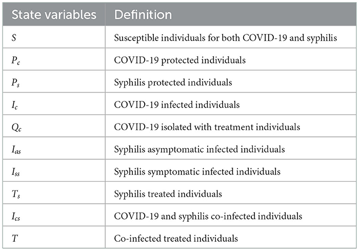
Table 1. Variables' definitions.

Assumptions and definitions of basic terms:

➢ Co-infectious humans do not transmit both infections simultaneously.

➢ COVID-19 infection is transmitted to susceptible individuals from I_c and I_cs infectious groups at the transmission rate as follows:

$\begin{array}{ll}{\lambda }_c={\beta }_2(I_c+{\varphi }_1{I}_{cs}).& (1)\end{array}$

➢ Syphilis infection is transmitted to susceptible individuals from I_as, I_ss, and I_cs infectious groups at the force of infection rate as follows:

$\begin{array}{ll}{\lambda }_s={\beta }_1(I_{as}+{\varphi }_2{I}_{ss}+{\varphi }_3{I}_{cs}).& (2)\end{array}$

Using variable and parameter definitions given in Tables 1, 2, respectively, the flowchart of the COVID-19 and syphilis co-infection model is represented in Figure 1.

TABLE 2

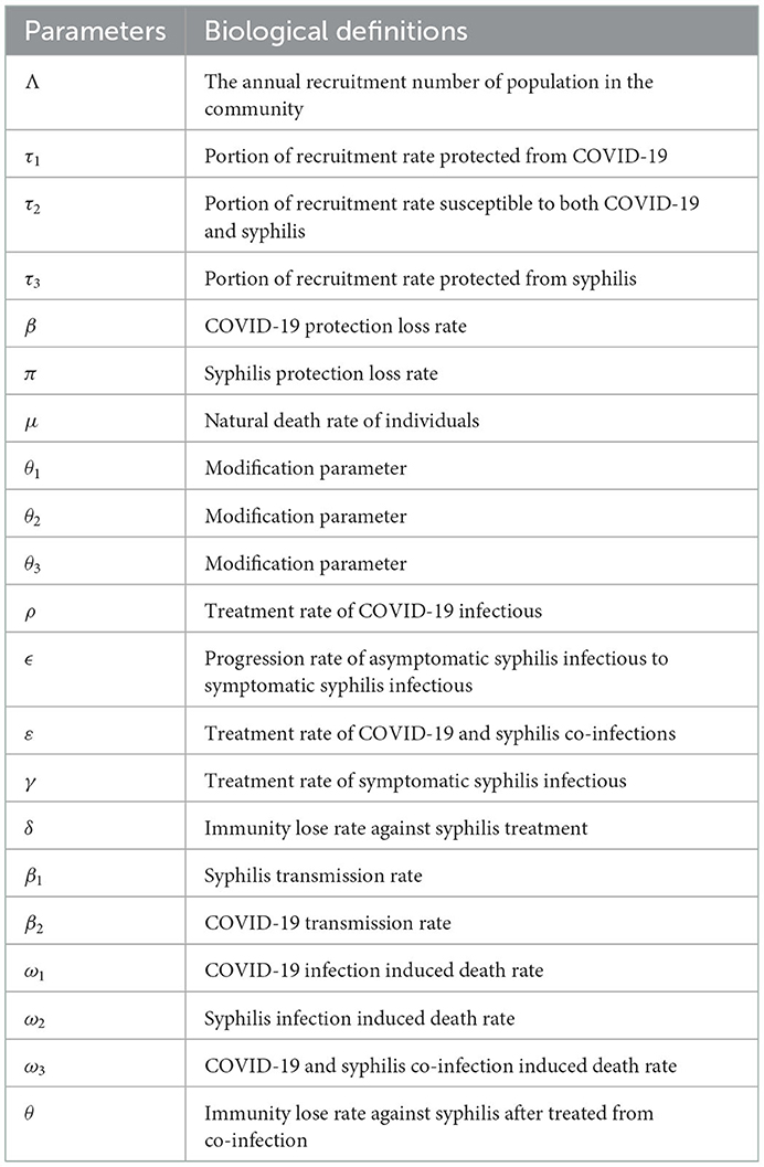
Table 2. Parameter definitions.

FIGURE 1

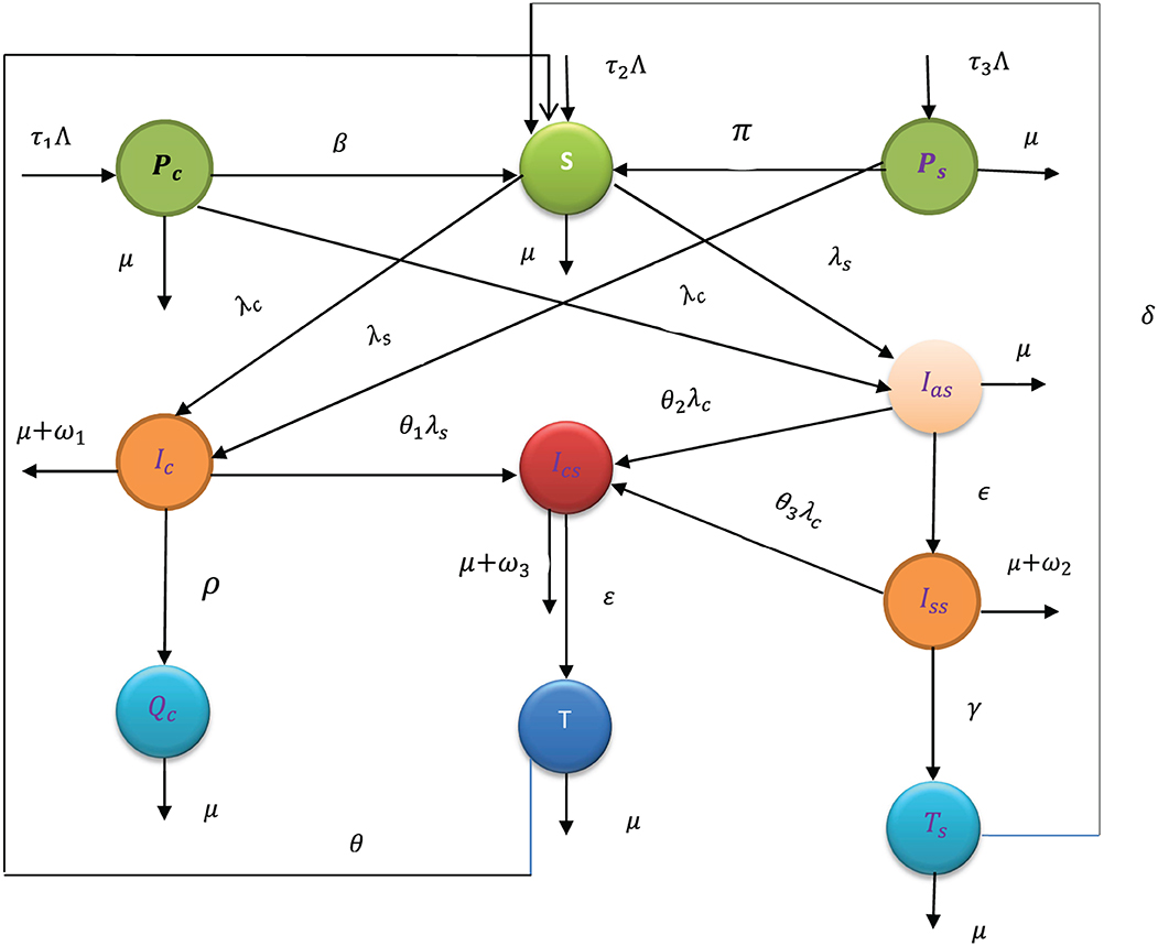
Figure 1. Flowchart of the model (3) with forces of infections λ_C and λ_s as in (1) and (2), respectively.

Using the flowchart represented in Figure 1, the corresponding system of differential equations of the complete co-infection model (3) is written as follows:

$\begin{array}{l}\frac{d{P}_c}{dt}={\tau }_1\Lambda -(\beta +{\lambda }_s+\mu )P_c,\\ \frac{d{P}_s}{dt}={\tau }_3\Lambda -(\pi +{\lambda }_c+\mu )P_s,\\ \frac{dS}{dt}={\tau }_2\Lambda +\beta P_c+\pi P_s+\delta T_s+\theta T-({\lambda }_s+{\lambda }_c+\mu )S,\\ \frac{d{I}_c}{dt}={\lambda }_{c}S+{\lambda }_c{P}_s-({\theta }_1{\lambda }_s+\rho +\mu +{\omega }_1)I_c,& (3)\\ \frac{d{Q}_c}{dt}=\rho I_c-\mu Q_c,\\ \frac{d{I}_{as}}{dt}={\lambda }_{s}S+{\lambda }_s{P}_c-({\theta }_2{\lambda }_c+ϵ+\mu )I_{as},\\ \frac{d{I}_{ss}}{dt}=ϵI_{as}-({\theta }_3{\lambda }_c+\gamma +\mu {+\omega }_2)I_{ss},\\ \frac{d{I}_{cs}}{dt}={\theta }_2{\lambda }_c{I}_{as}+{\theta }_3{\lambda }_c{I}_{ss}+{\theta }_1{\lambda }_s{I}_c-(\epsilon +\mu {+\omega }_3)I_{cs},\\ \frac{d{T}_s}{dt}=\gamma I_{ss}-(\delta +\mu )T_s,\\ \frac{dT}{dt}=\epsilon I_{cs}-(\theta +\mu )T.\end{array}$

2.1. Qualitative properties of the model (3)

System (3) represents the human population; we want to prove that all the solutions of the model are non-negative and bounded, respectively, in the following region:

$\begin{array}{ll}\Omega =\left\{\begin{array}{c}(P_c,P_s,S,I_c,Q_c,I_{as},I_{ss},T_s,T_{cs},T)\in {ℝ}_{+}^{10},N\le \frac{\Lambda }{\mu }\end{array}\right\}& (4)\end{array}$

Theorem 1: Let P_c(0) > 0, S(0) > 0, P_s(0), I_c(0) > 0, Q_c(0) > 0, I_as(0) > 0, I_ss(0) > 0, T_s(0) > 0, I_cs(0) > 0, T(0) > 0 be the initial solutions of the system (3), then P_c(t), P_s(t), S(t), I_c(t), Q_c(t), I_as(t), I_ss(t), T_s(t), T_cs(t), and T(t) are positive in the region ${ℝ}_{+}^{10}$ for any time t > 0.

Proof: Let τ = sup{t > 0:P_c(t) > 0, S(t) > 0, P_s(t), I_c(t) > 0, Q_c(t) > 0, I_as(t) > 0, I_ss(t) > 0, T_s(t) > 0, I_cs(t) > 0, T(t) > 0}.

Since P_c(t), P_s(t), S(t), I_c(t), Q_c(t), I_as(t), I_ss(t), T_s(t), T_cs(t), and T(t) are continuous, and we deduce that τ > 0. If τ = +∞, then positivity holds, but, if 0 < τ < +∞, P_c(τ) = 0 or P_s(τ) = 0 or S (τ) = 0 or I_c(τ) = 0 or Q_c(τ) = 0 or I_as(τ) = 0 I_ss(τ) = 0 or T_s(τ) = 0 or T_cs(τ) = 0 or T(τ) = 0.

From model (3) first equation, we do have

$\begin{array}{l}\frac{d{P}_c}{dt}+(\beta +{\lambda }_s+\mu )P_c={\tau }_1\Lambda .\end{array}$

After some calculations of integration, we got

$\begin{array}{l}{P}_c(\tau )=a_1{P}_c(0)+a_1{\displaystyle {\int }_0^{\tau }}{e}^{\int (\beta +{\lambda }_s+\mu )dt}{\tau }_1\Lambda dt>0,\text{ where}\\ a_1=e^{-\int (\beta +{\lambda }_s+\mu )dt}>0,P_c(0)>0,P_c(\tau )>0,\text{so that}\\ P_c(\tau )\ne 0.\end{array}$

From model (3) second equation, we have

$\begin{array}{l}\frac{d{P}_s}{dt}={\tau }_3\Lambda -(\pi +{\lambda }_c+\mu )P_s.\end{array}$

After some calculations of integration, we have

$\begin{array}{l}{P}_s(\tau )=b_1{P}_s(0)+b_1{\displaystyle {\int }_0^{\tau }}{e}^{\int (\pi +{\lambda }_c+\mu )dt}{\tau }_3\Lambda dt>0,\text{ where}\\ b_1=e^{-\int (\pi +{\lambda }_c+\mu )dt}>0,P_s(0)>0,P_s(\tau )>0,\text{so that}\\ P_s(\tau )\ne 0.\end{array}$

From model (3) third equation, we have

$\begin{array}{l}\frac{dS}{dt}={\tau }_2\Lambda +\beta P_c+\pi P_s+\delta \gamma T_s-S({\lambda }_s+{\lambda }_c+\mu ).\end{array}$

After some calculations, we have

$S(\tau )=c_{1}S(0)+c_1{\int }_0^{\tau }{e}^{\int ({\lambda }_s+{\lambda }_c+\mu )dt}({\tau }_2\Lambda +\beta P_c+\pi P_s+\delta \gamma T_s)dt>0$, where

$c_1=e^{-\int ({\lambda }_s+{\lambda }_c+\mu )dt}>0,S(0)>0$, and by the definition of τ we have P_c(t) > 0, P_s(t), T_s(t) > 0, S(τ) > 0, so that S(τ) ≠ 0.

Similarly, by proving the remaining state variable, we have

I_c(τ) > 0, hence I_c(τ) ≠ 0, Q_c(τ) > 0 hence Q_c(τ) ≠ 0, I_as(τ) > 0 hence I_as(τ) ≠ 0, I_ss(τ) > 0 hence I_ss(τ) ≠ 0,T_s(τ) > 0 hence T_s(τ) ≠ 0, T_cs(τ) > 0 hence T_cs(τ) ≠ 0, and T(τ) > 0 hence T(τ) ≠ 0.

Thus, τ is not finite, and hence = +∞, which means all the model solutions are non-negative.

Theorem 2: The model feasible region Ω stated in (4) is bounded in ${ℝ}_{+}^{10}$.

Proof: The total human being of the model (3) is as follows:

$\begin{array}{l}N(t)=P_c(t)+P_s(t)+S(t)+I_c(t)+Q_c(t)+I_{as}(t)\\ +I_{ss}(t)+T_s(t)+T_{cs}(t)+T(t).\end{array}$

Differentiating both sides gives the following result

$\begin{array}{l}\frac{dN}{dt}=\frac{d{P}_c}{dt}+\frac{d{P}_s}{dt}+\frac{dS}{dt}+\frac{d{I}_c}{dt}+\frac{d{Q}_c}{dt}+\frac{d{I}_{as}}{dt}+\frac{d{I}_{ss}}{dt}+\frac{d{T}_s}{dt}\\ +\frac{d{T}_{cs}}{dt}+\frac{dT}{dt}.\\ =\Lambda -\mu N-{\omega }_1{I}_c-{\omega }_2{I}_{ss}-{\omega }_3{I}_{cs},\text{where }{\tau }_1+{\tau }_3+{\tau }_2=1.\\ \Rightarrow \frac{dN}{dt}\le \Lambda -\mu N.\end{array}$

After some steps, we have $0\le N(t)\le \frac{\Delta }{\mu }$, and hence, the model solutions with positive initial solutions are bounded in Ω.

3. Model analysis in qualitative approach

The complete COVID-19 and syphilis co-infection model (3) depends on the results of the two sub-models analysis.

3.1. COVID-19 mono-infection model analysis

From the complete model (3), we have the COVID-19 mono-infection model taking values P_s = I_as = I_ss = T_s = I_cs = T = 0 as follows:

$\begin{array}{l}\frac{d{P}_c}{dt}={\tau }_1\Lambda -(\beta +\mu )P_c,\\ \frac{dS}{dt}={\tau }_2\Lambda +\beta P_c-({\lambda }_c+\mu )S,\\ \frac{d{I}_c}{dt}={\lambda }_{c}S-(\rho +\mu +{\omega }_1)I_c,& (5)\\ \frac{d{Q}_c}{dt}=\rho I_c-\mu Q_c.\end{array}$

with N₁(t) = P_c(t) + S(t) + I_c(t) + Q_c(t) as a total population and λ_c = β₂I_c.

3.1.1. COVID-19 infection-free equilibrium

The COVID-19 infection-free equilibrium of the model (5) at I_c = 0 is $E_c^0=\left(P_c^0,S^{0}0,0,0\right)=(\frac{{\tau }_1\Lambda }{\beta +\mu },\frac{{\tau }_2\Lambda \left(\beta +\mu \right)+\beta {\tau }_1\Lambda }{\mu \left(\beta +\mu \right)},0,0)$.

3.1.2. COVID-19 mono-infection reproduction number

This mono-infection model has one infectious class, I_c, and we can obtain basic reproduction numbers without a method of the next-generation matrix as follows:

$\begin{array}{l}\frac{d{I}_c}{dt}={\lambda }_{c}S-(\rho +\mu +{\omega }_1)I_c,\\ ={\beta }_2{I}_{c}S-(\rho +\mu +{\omega }_1)I_c,\\ =({\beta }_{2}S-(\rho +\mu +{\omega }_1))I_c,\\ =(\frac{{\beta }_2\Lambda ({\tau }_2(\beta +\mu )+\beta {\tau }_1)}{\mu (\beta +\mu )}-(\rho +\mu +{\omega }_1))I_c,\\ =(\rho +\mu +{\omega }_1)(\frac{{\beta }_2\Lambda ({\tau }_2(\beta +\mu )+\beta {\tau }_1)}{\mu (\beta +\mu )(\rho +\mu +{\omega }_1))}-1)I_c,\\ =(\rho +\mu +{\omega }_1)({\Re }_0^c-1)I_c,\text{where}\\ {\Re }_0^c=\frac{{\beta }_2{\tau }_2\Lambda (\beta +\mu )+{\beta }_2\beta {\tau }_1\Lambda }{\mu (\beta +\mu )(\rho +\mu +{\omega }_1)}.\end{array}$

3.1.3. COVID-19 incidence equilibrium point

The COVID-19 incidence equilibrium point of the system (5) is $E_c^{*}=(P_c^{*},S^{*},I_c^{*},Q_c^{*})$, where

$\begin{array}{l}{P}_c^{*}=\frac{{\tau }_1\Lambda }{\beta +\mu },S^{*}=\frac{{\tau }_3\Lambda (\beta +\mu )+{\tau }_1\beta \Lambda ,}{({\lambda }_c^{*}+\mu )(\beta +\mu )},\\ I_c^{*}=\frac{({\tau }_3\Lambda (\beta +\mu )+{\tau }_1\beta \Lambda ){\lambda }_c^{*}}{({\lambda }_c^{*}+\mu )(\beta +\mu )(\rho +\mu +{\omega }_1)},\\ Q_c^{*}=\frac{({\tau }_3\Lambda (\beta +\mu )+{\tau }_1\beta \Lambda )\rho {\lambda }_c^{*}}{\mu ({\lambda }_c^{*}+\mu )(\beta +\mu )(\rho +\mu +{\omega }_1)}.\end{array}$

Theorem 3: The COVID-19 mono-infection model (5) has a unique COVID-19 incidence (endemic) equilibrium point whenever${\Re }_0^c>1$.

Proof: Using equation (1), we have the following:

$\begin{array}{l}{\lambda }_c^{*}={\beta }_1{I}_c^{*}=\frac{{\beta }_1({\tau }_3\Lambda (\beta +\mu )+{\tau }_1\beta \Lambda ){\lambda }_c^{*}}{({\lambda }_c^{*}+\mu )(\beta +\mu )(\rho +\mu +{\omega }_1)}.\end{array}$

Then the non-zero value of ${\lambda }_c^{*}$ after a simple simplification is as follows:

${\lambda }_c^{*}=\mu ({{R}}_0^c-1)>0$, if and only if ${{R}}_0^c>1$.

Hence, the COVID-19 mono-infection model (5) has a unique incidence equilibrium point if and only if ${{R}}_0^c>1$.

Theorem 4: COVID-19 infection-free equilibrium point of the model (5) is locally asymptotically stable if${\Re }_0^c<1$; otherwise, it is unstable.

Proof: The Jacobean matrix of the model (5) at the COVID-19 infection-free equilibrium point is

$\begin{array}{l}J(E_c^0)=\left(\begin{array}{cccc}-(\beta +\mu )& 0& 0& 0\\ \beta & -\mu & \frac{-{\beta }_2({\tau }_2\Lambda (\beta +\mu )+\beta {\tau }_1\Lambda )}{\mu (\beta +\mu )}& 0\\ 0& 0& \frac{{\beta }_2({\tau }_2\Lambda (\beta +\mu )+\beta {\tau }_1\Lambda )-\mu (\beta +\mu )(\rho +\mu +{\omega }_1)}{\mu (\beta +\mu )}& 0\\ 0& 0& \rho & -\mu \end{array}\right).\end{array}$

Further, the characteristics equation after a certain calculation gives us as follows:

$\begin{array}{l}{\lambda }_1=-(\beta +\mu )<0or{\lambda }_2=-\mu <0,\text{or}\\ {\lambda }_3=(\rho +\mu +{\omega }_1)({{R}}_0^c-1).\end{array}$

Thus, each eigenvalue of the Jacobian matrix is negative if ${{R}}_0^c<1$ implies the COVID-19 infection-free equilibrium point is locally asymptotically stable whenever ${{R}}_0^c<1.$

Theorem 5: The COVID-19 infection-free equilibrium point denoted by $E_c^{*}$ of the COVID-19 mono-infection model is globally stable if ${{R}}_0^c<1$; otherwise, it is unstable.

Proof: Take the representative Lyapunov function l(I_c ) = aI_c, where $a=\frac{1}{\left(\rho +\mu +{\omega }_1\right))}$,

$\begin{array}{l}l\left(I_c\right)=a{I}_c=\frac{1}{(\rho +\mu +{\omega }_1)}{I}_c,\\ \frac{dl}{dt}=\frac{1}{(\rho +\mu +{\omega }_1)}(({\beta }_{2}S-(\rho +\mu +{\omega }_1))I_c),\\ \le \frac{1}{(\rho +\mu +{\omega }_1)}\\ (\frac{{\beta }_2\Lambda ({\tau }_2(\beta +\mu )+\beta {\tau }_1)-\mu (\beta +\mu )(\rho +\mu +{\omega }_1)}{\mu (\beta +\mu )})I_c,\\ \le (\frac{{\beta }_2\Lambda ({\tau }_2(\beta +\mu )+\beta {\tau }_1)-\mu (\beta +\mu )(\rho +\mu +{\omega }_1)}{\mu (\beta +\mu )(\rho +\mu +{\omega }_1)})I_c,\\ \le \mu (\beta +\mu )(\rho +\mu +{\omega }_1)(\frac{\frac{{\beta }_2\Lambda ({\tau }_2(\beta +\mu )+\beta {\tau }_1)}{\mu (\beta +\mu )(\rho +\mu +{\omega }_1)}-1}{\mu (\beta +\mu )(\rho +\mu +{\omega }_1)})I_c,\\ \le \mu (\beta +\mu )(\rho +\mu +{\omega }_1)(\frac{{{R}}_0^c-1}{\mu (\beta +\mu )(\rho +\mu +{\omega }_1)})I_c,\\ \le ({{R}}_0^c-1)I_c.\end{array}$

Thus, $\frac{dl}{dt}<0$, if ${{R}}_0^c<1$, and the equality $\frac{dl}{dt}=0$ holds if ${{R}}_0^c=1$, and hence the COVID-19 infection-free equilibrium point is globally asymptotically stable if ${{R}}_0^c<1.$

Theorem 6: The COVID-19 incidence denoted by $E_C^{*}$ of the COVID-19 mono-infection model (5) is locally asymptotically stable whenever${{R}}_0^c>1$; otherwise, it is unstable.

Proof: The Jacobean of the system (5) at $E_C^{*}$

$\begin{array}{l}J\left(E_C^{\ast }\right)=\left(\begin{array}{cccc}-\left(\beta +\mu \right)& 0& 0& 0\\ \beta & -\left({\beta }_2{I}_c{}^{*}+\mu \right)& -{\beta }_2{S}^{\ast }& 0\\ 0& {\beta }_2{I}_c^{*}& {\beta }_2{S}^{*}-\left(\rho +\mu +{\omega }_1\right)& 0\\ 0& 0& \rho & -\mu \end{array}\right).\end{array}$

From the Jacobean matrix, the characteristics equation, after simplification, gives as follows:

$\begin{array}{l}\left(-\left(\beta +\mu \right)-\lambda \right)(-\mu -\lambda )[\left(-\left({\beta }_2{I}_c^{\ast }+\mu \right)-\lambda \right)({\beta }_2{S}^{*}-(\rho +\mu \\ +{\omega }_1)-\lambda )+{\beta }_2{S}^{\ast }{\beta }_2{I}_c^{\ast }]=0.\end{array}$

Then we do have the eigenvalues λ₁ = −μ < 0 or λ₂ = −(β + μ) < 0 or

$\begin{array}{l}{a}_0{\lambda }^2+a_1\lambda +a_2=0where\\ a_0\text{= 1,}\\ a_1=\left(\frac{\begin{array}{l}{\beta }_2\left({\tau }_3\Lambda \left(\beta +\mu \right)+{\tau }_1\beta \Lambda \right)\mu ({{R}}_0^c-1)\hfill \\ +\mu ({\lambda }_c^{\ast }+\mu )(\beta +\mu )(\rho +\mu +{\omega }_1)\hfill \end{array}}{({\lambda }_c^{\ast }+\mu )(\beta +\mu )(\rho +\mu +{\omega }_1)}\right)\\ +\frac{({\beta }_2{\tau }_2\Lambda (\beta +\mu )+{\tau }_1\beta \Lambda )[({\lambda }_c^{\ast }+\mu )\mu {{R}}_0^c-1]}{({\lambda }_c^{\ast }+\mu )(\beta +\mu )},\\ a_2=\frac{{\beta }_2({\tau }_3\Lambda (\beta +\mu )+{\tau }_1\beta \Lambda )\mu ({{R}}_0^c-1)}{({\lambda }_c^{\ast }+\mu )(\beta +\mu )(\rho +\mu +{\omega }_1)}\\ +\frac{({\beta }_2{\tau }_2\Lambda (\beta +\mu )+{\tau }_1\beta \Lambda )[({\lambda }_c^{\ast }+\mu )\mu {{R}}_0^c-1]}{({\lambda }_c^{\ast }+\mu )(\beta +\mu )}\\ +\frac{{\beta }_2({\tau }_2\Lambda (\beta +\mu )+{\tau }_1\beta \Lambda )\mu ({{R}}_0^c-1)}{({\lambda }_c^{\ast }+\mu )(\beta +\mu )(\rho +\mu +{\omega }_1)}.\end{array}$

Hence, all the coefficients of the characteristics equations are positive when ${{R}}_0^c>1;$ thus, the COVID-19 incidence equilibrium point has local asymptotic stability when ${{R}}_0^c>1$.

3.2. Analysis of syphilis sub-model

The syphilis sub-model is obtained from the system (3) by making P_c = I_c = Q_c = I_cs = T = 0 and is as follows:

$\begin{array}{l}\frac{d{P}_s}{dt}={\tau }_3\Lambda -(\pi +\mu )P_s,\\ \frac{dS}{dt}={\tau }_2\Lambda +\pi P_s+\delta \gamma T_s-S({\lambda }_s+\mu ),\\ \frac{d{I}_{as}}{dt}={\lambda }_{s}S-I_{as}(ϵ+\mu ),& (6)\\ \frac{d{I}_{ss}}{dt}=ϵI_{as}-I_{ss}(\gamma +\mu {+\omega }_2),\\ \frac{d{T}_s}{dt}=\gamma I_{ss}-T_s(\delta \gamma +\mu ).\end{array}$

With N₂(t) = P_s(t) + S(t) + I_as(t) + I_ss(t) + T_s(t), and λ_s = β₁(I_as + ϕ₂I_ss ).

3.2.1. Syphilis infection-free equilibrium

The syphilis infection-free equilibrium point of the model (6) was obtained by making I_as = I_ss = 0 and is given by $E_s^0=(P_s^0,S^0,I_{as}^0,I_{ss}^0,T_s^0)=\left(\frac{{\tau }_3\Lambda }{\pi +\mu },\frac{{\tau }_2\Lambda (\pi +\mu )+{\tau }_3\pi \Lambda }{\mu (\pi +\mu )},0,0,0\right).$

3.2.2. Syphilis sub-model reproduction number

The syphilis sub-model (6) has two infectious classes, which are I_as, and I_ss, then applying the next-generation matrix method stated in [43, 44] to obtain the basic reproduction number of the system (6) by computing FV⁻¹ as follows:

$\begin{array}{l}F=\left(\begin{array}{cc}{\beta }_1{S}^0& {\beta }_1{\varphi }_2{S}^0\\ 0& 0\end{array}\right),\\ \Rightarrow F=\left(\begin{array}{cc}\frac{{\beta }_1\Lambda ({\tau }_2(\pi +\mu )+{\tau }_3\pi )}{\mu (\pi +\mu )}& \frac{{\beta }_1{\varphi }_2\Lambda ({\tau }_2(\pi +\mu )+{\tau }_3\pi )}{\mu (\pi +\mu )}\\ 0& 0\end{array}\right),\end{array}$

and

$\begin{array}{l}V=\left(\begin{array}{cc}ϵ+\mu & 0\\ -ϵ& \gamma +\mu {+\omega }_2\end{array}\right).\end{array}$

Then, we applied Mathematica coding; we have

$\begin{array}{l}{V}^{-1}=\left[\begin{array}{cc}\frac{1}{ϵ+\mu }& 0\\ \frac{ϵ}{(\gamma +\mu +{\omega }_2)(ϵ+\mu )}& \frac{1}{(\gamma +\mu +{\omega }_2)}\end{array}\right],\text{ and}\\ F{V}^{-1}=[\frac{{\beta }_1\Lambda ({\tau }_2(\pi +\mu )+{\tau }_3\pi )}{\mu \left(\pi +\mu \right)(ϵ+\mu )}\\ +\begin{array}{cc}\frac{ϵ{\beta }_1{\varphi }_2\Lambda \left({\tau }_2\left(\pi +\mu \right)+{\tau }_3\pi \right)}{\mu \left(\pi +\mu \right)(\gamma +\mu +{\omega }_2)\left(ϵ+\mu \right)}& \frac{{\beta }_1{\varphi }_2\Lambda \left({\tau }_2\left(\pi +\mu \right)+{\tau }_3\pi \right)}{\mu \left(\pi +\mu \right)(\gamma +\mu +{\omega }_2)}\\ 0& 0\end{array}].\end{array}$

Thus, the reproduction number of the syphilis sub-model (6) is given by ${{R}}_0^s=\frac{{\beta }_1\Lambda \left[(\gamma +\mu {+\omega }_2)+{\varphi }_2ϵ\right]({\tau }_2(\pi +\mu )+{\tau }_3\pi )}{\mu (\pi +\mu )(\gamma +\mu {+\omega }_2)(ϵ+\mu )}$.

3.2.3. Syphilis incidence equilibrium point of the system (6)

Making the model (6) equation to zero, we have the syphilis incidence equilibrium point given by $E_s^{*}=(P_s^{*},S^{*},I_{as}^{*},I_{ss}^{*},T_s^{*})$, where

$\begin{array}{l}{P}_s^{*}=\frac{{\tau }_3\Lambda }{(\pi +\mu )},\\ S^{*}=\frac{(\gamma +\mu {+\omega }_2)(ϵ+\mu )(\delta \gamma +\mu )({\tau }_2\Lambda (\pi +\mu )+{\tau }_3\Lambda \pi )}{(\pi +\mu )((\gamma +\mu {+\omega }_2)(ϵ+\mu )({\lambda }_s+\mu )(\delta \gamma +\mu )-\gamma \delta \gamma ϵ{\lambda }_s)},\\ I_{as}^{*}=\frac{{\lambda }_s(\gamma +\mu {+\omega }_2)(\delta \gamma +\mu )({\tau }_2\Lambda (\pi +\mu )+{\tau }_3\Lambda \pi )}{(\pi +\mu )((\gamma +\mu {+\omega }_2)(ϵ+\mu )({\lambda }_s+\mu )(\delta \gamma +\mu )-\gamma \delta \gamma ϵ{\lambda }_s)},\\ I_{ss}^{*}=\frac{ϵ{\lambda }_s(\delta \gamma +\mu )({\tau }_2\Lambda (\pi +\mu )+{\tau }_3\Lambda \pi )}{(\pi +\mu )((\gamma +\mu {+\omega }_2)(ϵ+\mu )({\lambda }_s+\mu )(\delta \gamma +\mu )-\gamma \delta \gamma ϵ{\lambda }_s)},\\ T_s^{*}=\frac{ϵ{\lambda }_s\gamma ({\tau }_2\Lambda (\pi +\mu )+{\tau }_3\Lambda \pi )}{(\pi +\mu )((\gamma +\mu {+\omega }_2)(ϵ+\mu )({\lambda }_s+\mu )(\delta \gamma +\mu )-\gamma \delta \gamma ϵ{\lambda }_s)}.\end{array}$

Theorem 7: The syphilis incidence equilibrium point of syphilis in the model (6) is unique whenever ${{R}}_s^0>1.$

Proof: From the syphilis infection rate, we have

$\begin{array}{l}{\lambda }_s^{\ast }={\beta }_1(I_{as}^{\ast }+{\varphi }_2{I}_{ss}^{\ast }).\\ {\lambda }_s^{\ast }={\beta }_1(\frac{{\lambda }_s(\gamma +\mu +{\omega }_2)(\delta \gamma +\mu )({\tau }_2\Lambda \left(\pi +\mu \right)+{\tau }_3\Lambda \pi )}{\begin{array}{c}\left(\pi +\mu \right)((\gamma +\mu +{\omega }_2)\left(ϵ+\mu \right)\left({\lambda }_s^{\ast }+\mu \right)\left(\delta \gamma +\mu \right)\\ -ϵ\gamma \delta \gamma {\lambda }_s^{\ast })\end{array}}\\ +\frac{ϵ{\lambda }_s^{\ast }{\varphi }_2(\delta \gamma +\mu )({\tau }_2\Lambda \left(\pi +\mu \right)+{\tau }_3\Lambda \pi )}{\begin{array}{c}\left(\pi +\mu \right)((\gamma +\mu +{\omega }_2)\left(ϵ+\mu \right)\left({\lambda }_s^{\ast }+\mu \right)\left(\delta \gamma +\mu \right)\\ -\gamma \delta \gamma ϵ{\lambda }_s^{\ast })\end{array}}).\\ \Rightarrow {\lambda }_s^{\ast }=\left(\delta \gamma +\mu \right)\\ \frac{\begin{array}{c}{\beta }_1\Lambda [(\gamma +\mu +{\omega }_2)\left({\tau }_2\left(\pi +\mu \right)+{\tau }_3\pi \right)+ϵ{\varphi }_2({\tau }_2\left(\pi +\mu \right)\\ +{\tau }_3\pi )]-\mu \left(\pi +\mu \right)[(\gamma +\mu +{\omega }_2)\left(ϵ+\mu \right)]\end{array}}{\left(\pi +\mu \right)\left((\gamma +\mu +{\omega }_2)\left(ϵ+\mu \right)\left(\delta \gamma +\mu \right)-\gamma \delta \gamma ϵ\right)}.\\ \Rightarrow {\lambda }_s^{\ast }=\frac{\left(\delta \gamma +\mu \right)\mu (\gamma +\mu +{\omega }_2)\left(ϵ+\mu \right)({{R}}_0^s-1)}{\left((\gamma +\mu +{\omega }_2)\left(ϵ+\mu \right)\left(\delta \gamma +\mu \right)-\gamma \delta \gamma ϵ\right)}.\\ \Rightarrow {\lambda }_s^{\ast }={\text{k}}_1({{R}}_0^s-1),\text{where}\\ {\text{k}}_1=\frac{\left(\delta \gamma +\mu \right)\mu \left(\pi +\mu \right)(\gamma +\mu +{\omega }_2)\left(ϵ+\mu \right)}{\left(\pi +\mu \right)\left((\gamma +\mu +{\omega }_2)\left(ϵ+\mu \right)\left(\delta \gamma +\mu \right)-\gamma \delta \gamma ϵ\right)}.\end{array}$

Hence, the syphilis sub-model (6) has a unique incidence equilibrium if ${{R}}_0^s>1$.

Theorem 8: Syphilis infection-free equilibrium point of the model (3) has local asymptotic stability if${{R}}_0^s<1$; otherwise, it is unstable.

Proof: Jacobean of the model (6) at the syphilis infection-free equilibrium point is as follows:

$\begin{array}{l}J(E_0^s)=\left(\begin{array}{ccccc}-(\pi +\mu )& 0& 0& 0& 0\\ \pi & -\mu & \frac{-{\beta }_1\Lambda ({\tau }_2(\pi +\mu )+{\tau }_3\pi )}{\mu (\pi +\mu )}& \frac{-{\beta }_1{\varphi }_2\Lambda ({\tau }_2(\pi +\mu )+{\tau }_3\pi )}{\mu (\pi +\mu )}& \delta \gamma \\ 0& 0& \frac{{\beta }_1\Lambda ({\tau }_2(\pi +\mu )+{\tau }_3\pi )-\mu (\pi +\mu )(ϵ+\mu )}{\mu (\pi +\mu )}& \frac{{\beta }_1{\varphi }_2\Lambda ({\tau }_2(\pi +\mu )+{\tau }_3\pi )}{\mu (\pi +\mu )}& 0\\ 0& 0& ϵ& -(\gamma +\mu {+\omega }_2)& 0\\ 0& 0& 0& \gamma & -(\delta \gamma +\mu )\end{array}\right).\end{array}$

From the Jacobian matrix, the characteristics equation after simplification is as follows:

$\begin{array}{l}\left(-\left(\pi +\mu \right)\lambda \right)\left(-\mu -\lambda \right)(-\left(\delta \gamma +\mu \right)\lambda )\\ [\left(\frac{{\beta }_1\Lambda \left({\tau }_2\left(\pi +\mu \right)+{\tau }_3\pi \right)-\mu \left(\pi +\mu \right)\left(ϵ+\mu \right)}{\mu \left(\pi +\mu \right)}\lambda \right)\\ (-(\gamma +\mu +{\omega }_2)\lambda )-(\frac{{\beta }_1{\varphi }_2\Lambda ϵ\left({\tau }_2\left(\pi +\mu \right)+{\tau }_3\pi \right)}{\mu \left(\pi +\mu \right)})]=0.\end{array}$

Then the eigenvalues are λ₁ = −(π + μ) < 0 or λ₂ = −μ < 0 or λ₃ = −(δγ + μ) < 0 or $a_0{\lambda }^2+a_1\lambda +a_2=0$.

where,

$\begin{array}{l}{a}_0=1,\\ a_1=(\gamma +\mu {+\omega }_2)+(ϵ+\mu )+\frac{{\beta }_1\Lambda ({\tau }_2(\pi +\mu )+{\tau }_3\pi )}{\mu (\pi +\mu )},\\ a_2=(ϵ+\mu )(\gamma +\mu {+\omega }_2)(1-{{R}}_0^s).\end{array}$

Applying Routh–Hurwitz criteria stated in [33], each eigenvalue of the matrix is negative whenever${{R}}_0^s<1$; thus, the syphilis infection-free equilibrium point has local asymptotic stability if ${{R}}_0^s<1$.

Theorem 9: Syphilis infection-free equilibrium point $E_s^0$ of the model (6) has global stability if ${{R}}_0^s<1$; otherwise, it is unstable.

Proof: Let the Lyapunov representative function be given as l(I_as, I_ss ) = aI_as + bI_ss, where $=\frac{\left[(\gamma +\mu )+{\varphi }_2ϵ\right]}{(ϵ+\mu )(\gamma +\mu {+\omega }_2)}$, $b=\frac{{\varphi }_2}{(\gamma +\mu {+\omega }_2)}$.

$\begin{array}{l}\Rightarrow l(I_{as},I_{ss})=\frac{[(\gamma +\mu {+\omega }_2)+{\varphi }_2ϵ]}{(ϵ+\mu )(\gamma +\mu {+\omega }_2)}{I}_{as}+\frac{{\varphi }_2}{(\gamma +\mu {+\omega }_2)}{I}_{ss}.\\ \Rightarrow \frac{dl}{dt}=\frac{[(\gamma +\mu {+\omega }_2)+{\varphi }_2ϵ]}{(ϵ+\mu )(\gamma +\mu {+\omega }_2)}({\lambda }_{s}S-I_{as}(ϵ+\mu ))\\ +\frac{{\varphi }_2}{(\gamma +\mu )}(ϵI_{as}-I_{ss}(\gamma +\mu {+\omega }_2)),\\ \le \frac{[(\gamma +\mu {+\omega }_2)+{\varphi }_2ϵ]}{(ϵ+\mu )(\gamma +\mu {+\omega }_2)}({\beta }_1(I_{as}+{\varphi }_2{I}_{ss})S^{*}-I_{as}(ϵ+\mu ))\\ +\frac{{\varphi }_2}{(\gamma +\mu )}(ϵI_{as}-I_{ss}(\gamma +\mu {+\omega }_2)),\\ \le \frac{[(\gamma +\mu {+\omega }_2)+{\varphi }_2ϵ]}{(ϵ+\mu )(\gamma +\mu {+\omega }_2)}({\beta }_1{I}_{as}{S}^{*}+{\beta }_1{\varphi }_2{I}_{ss}{S}^{*}-I_{as}(ϵ+\mu ))\\ +\frac{{\varphi }_2}{(\gamma +\mu )}(ϵI_{as}-I_{ss}(\gamma +\mu {+\omega }_2)),\\ \le ([{\beta }_1{S}^{*}-(ϵ+\mu )]\frac{[(\gamma +\mu {+\omega }_2)+{\varphi }_2ϵ]}{(ϵ+\mu )(\gamma +\mu {+\omega }_2)}+\frac{{\varphi }_2ϵ}{(\gamma +\mu {+\omega }_2)})I_{as}\\ +(\frac{{\beta }_1{\varphi }_2[(\gamma +\mu {+\omega }_2)+{\varphi }_2ϵ]S^{*}}{(ϵ+\mu )(\gamma +\mu {+\omega }_2)}-{\varphi }_2)I_{ss},\\ \le ([\frac{[(\gamma +\mu )+{\varphi }_2ϵ]{\beta }_1{S}^{*}}{(ϵ+\mu )(\gamma +\mu {+\omega }_2)}-\frac{[(\gamma +\mu {+\omega }_2)+{\varphi }_2ϵ]}{(\gamma +\mu {+\omega }_2)}])I_{as}\\ +(\frac{{\beta }_1{\varphi }_2[(\gamma +\mu {+\omega }_2)+{\varphi }_2ϵ]S^{*}}{(ϵ+\mu )(\gamma +\mu {+\omega }_2)}-{\varphi }_2)I_{ss},\\ \le \frac{[(\gamma +\mu {+\omega }_2)+{\varphi }_2ϵ]{\beta }_1\Lambda ({\tau }_2(\pi +\mu )+{\tau }_3\pi )}{\mu (\pi +\mu )(ϵ+\mu )(\gamma +\mu {+\omega }_2)}{I}_{as}\\ -\frac{[(\gamma +\mu {+\omega }_2)+{\varphi }_2ϵ]}{(\gamma +\mu {+\omega }_2)}{I}_{as}+\\ (\frac{{\beta }_1{\varphi }_2[(\gamma +\mu {+\omega }_2)+{\varphi }_2ϵ]\Lambda ({\tau }_2(\pi +\mu )+{\tau }_3\pi )}{\mu (\pi +\mu )(ϵ+\mu )(\gamma +\mu {+\omega }_2)}-{\varphi }_2)I_{ss}.\\ \le ([\frac{[(\gamma +\mu {+\omega }_2)+{\varphi }_2ϵ]{\beta }_1\Lambda ({\tau }_2(\pi +\mu )+{\tau }_3\pi )}{\mu (\pi +\mu )(ϵ+\mu )(\gamma +\mu {+\omega }_2)}-m])I_{as}\\ +(\frac{{\beta }_1{\varphi }_2[(\gamma +\mu {+\omega }_2)+{\varphi }_2ϵ]\Lambda ({\tau }_2(\pi +\mu )+{\tau }_3\pi )}{\mu (\pi +\mu )(ϵ+\mu )(\gamma +\mu {+\omega }_2)}-{\varphi }_2),where\\ m=\frac{[(\gamma +\mu {+\omega }_2)+{\varphi }_2ϵ]}{(\gamma +\mu {+\omega }_2)}>1.\\ \le m([\frac{{{R}}_0^s}{m}-1])I_{as}+{\varphi }_2(\frac{{{R}}_0^s}{{\varphi }_2}-1)I_{ss},\\ \frac{{{R}}_0^s}{m}<1,\frac{{{R}}_s^0}{{\varphi }_2}<1,\\ \frac{{{R}}_0^s}{m}<1,\frac{{{R}}_0^s}{{\varphi }_2}<1\text{ implies }{{R}}_0^s<1\text{ since m}\\ =\frac{[(\gamma +\mu {+\omega }_2)+{\varphi }_2ϵ]}{(\gamma +\mu {+\omega }_2)}>1,\text{ and }{\varphi }_2>1.\end{array}$

Hence, the syphilis-free equilibrium point is globally stable if ${{R}}_0^s<1$.

3.3. COVID-19 and syphilis co-infection model analysis

3.3.1. The model (3) disease-free equilibrium

Making all the equations of (3) zero with I_c = I_as = I_ss = I_cs = 0, the disease-free equilibrium point of (3) is given by $E^0=\left(P_c^0,P_s^0,S^0,I_c^0,Q_c^0,I_{as}^0,I_{ss}^0,T_s^0,T_{cs}^0,T^0\right)=$ $(\frac{{\tau }_1\Lambda }{\left(\beta +\mu \right)},\frac{{\tau }_3\Lambda }{(\pi +\mu )},\frac{\Lambda ({\tau }_2\left(\beta +\mu \right)\left(\pi +\mu \right)+{\tau }_1\beta \left(\pi +\mu \right)+{\tau }_3\pi \left(\beta +\mu \right))}{\mu \left(\beta +\mu \right)(\pi +\mu )},0,0,0,0,0,0,0)$.

3.3.2. The model (3) reproduction number

The COVID-19 and syphilis co-infection model (3) reproduction number denoted by ${\Re }_0^{cs}$ is calculated using next-generation matrix criteria, as stated in [44]. Since we have four infectious groups, those are I_c, I_as, I_ss, and I_cs, and we have

$\begin{array}{l}{f}_i=\left[\begin{array}{c}{\beta }_2(I_c+{\varphi }_1{I}_{cs})(S+P_s)\\ {\beta }_1(I_{as}+{\varphi }_2{I}_{ss}+{\varphi }_3{I}_{cs})(S+P_c)\\ 0\\ {\beta }_2({\theta }_2{I}_{as}+{\theta }_3{I}_{ss})(I_c+{\varphi }_1{I}_{cs})+{\theta }_1{\beta }_1(I_{as}+{\varphi }_2{I}_{ss}+{\varphi }_3{I}_{cs})I_c\end{array}\right].\\ \Rightarrow f=\left[\begin{array}{cccc}{\beta }_2(S^0+P_s^0)& 0& 0& {\varphi }_1(S^0+P_s^0)\\ 0& {\beta }_1(S^0+P_c^0)& {\beta }_1{\varphi }_2(S^0+P_c^0)& {\beta }_1{\varphi }_3(S^0+P_c^0)\\ 0& 0& 0& 0\\ 0& 0& 0& 0\end{array}\right],\end{array}$

and

$\begin{array}{l}{v}_i={v_i}^{-}(x)-{v_i}^{+}(x)\\ =\left[\begin{array}{c}{I}_c({\theta }_1{\beta }_1(I_{as}+{\varphi }_2{I}_{ss}+{\varphi }_3{I}_{cs})+\rho +\mu {+\omega }_1)\\ I_{as}({\theta }_2{\beta }_2(I_c+{\varphi }_1{I}_{cs})+ϵ+\mu )\\ I_{ss}({\theta }_3{\beta }_2(I_c+{\varphi }_1{I}_{cs})+\gamma +\mu {+\omega }_2)-ϵI_{as}\\ I_{cs}(\epsilon +\mu {+\omega }_3)\end{array}\right].\\ \Rightarrow v=\left[\begin{array}{cccc}(\rho +\mu {+\omega }_1)& 0& 0& 0\\ 0& (ϵ+\mu )& 0& 0\\ 0& -ϵ& (\gamma +\mu {+\omega }_2)& 0\\ 0& 0& 0& (\epsilon +\mu {+\omega }_3)\end{array}\right].\end{array}$

Then applying Mathematica, we have got

$\begin{array}{l}{v}^{-1}=\left[\begin{array}{cccc}\frac{1}{(\rho +\mu {+\omega }_1)}& 0& 0& 0\\ 0& \frac{1}{(\epsilon +\mu )}& 0& 0\\ 0& 0& \frac{1}{(\gamma +\mu {+\omega }_2)}& 0\\ 0& 0& 0& \frac{1}{(\epsilon +\mu {+\omega }_3)}\end{array}\right],\end{array}$

and

$\begin{array}{l}f{v}^{-1}=\left[\begin{array}{cccc}\frac{{\beta }_2(S^0+{P^0}_s)}{(\rho +\mu {+\omega }_1)}& 0& 0& \frac{{\varphi }_1(S^0+{P^0}_s)}{(\epsilon +\mu {+\omega }_3)}\\ 0& \frac{{\beta }_1(S^0+{P^0}_c)}{(\epsilon +\mu )}& \frac{{\beta }_1{\varphi }_2(S^0+{P^0}_c)}{(\gamma +\mu {+\omega }_2)}& \frac{{\beta }_1{\varphi }_3(S^0+{P^0}_c)}{(\epsilon +\mu {+\omega }_3)}\\ 0& 0& 0& 0\\ 0& 0& 0& 0\end{array}\right].\\ \Rightarrow \left|\begin{array}{cccc}\frac{{\beta }_2(S^0+{P^0}_s)}{(\rho +\mu {+\omega }_1)}-\lambda & 0& 0& \frac{{\varphi }_1(S^0+{P^0}_s)}{(\epsilon +\mu {+\omega }_3)}\\ 0& \frac{{\beta }_1(S^0+{P^0}_c)}{(\epsilon +\mu )}-\lambda & \frac{{\beta }_1{\varphi }_2(S^0+{P^0}_c)}{(\gamma +\mu {+\omega }_2)}& \frac{{\beta }_1{\varphi }_3(S^0+{P^0}_c)}{(\epsilon +\mu {+\omega }_3)}\\ 0& 0& 0-\lambda & 0\\ 0& 0& 0& 0-\lambda \end{array}\right|\\ =0.\end{array}$

Then, the corresponding eigenvalues are λ₁ = 0 or λ₂ = 0 or ${\lambda }_3=\frac{{\beta }_2(S^0+{P^0}_s)}{(\rho +\mu {+\omega }_1)}=\frac{{\beta }_2\Lambda {\tau }_2}{\mu (\rho +\mu {+\omega }_1)}+\frac{{\beta }_2\Lambda {\tau }_1\beta }{\mu (\beta +\mu )(\rho +\mu {+\omega }_1)}+\frac{{\beta }_2\Lambda {\tau }_3}{\mu (\rho +\mu {+\omega }_1)}={\Re }_0^c+n$ or ${\lambda }_4={\beta }_1(\frac{{\tau }_2\Lambda (\beta +\mu )(\pi +\mu )+{\tau }_1\beta \Lambda (\pi +\mu )+{\tau }_3\pi \Lambda (\beta +\mu )+{\tau }_1\Lambda \mu (\pi +\mu )}{\mu (\beta +\mu )(\pi +\mu )(\epsilon +\mu )})$ $={\Re }_0^s-m$ where $,n=\frac{{\beta }_2\Lambda {\tau }_3}{\mu (\rho +\mu {+\omega }_1)}$, $m=\frac{{\beta }_1\Lambda \left[ϵ{\varphi }_2({\tau }_2(\pi +\mu )+{\tau }_3\pi )-{\tau }_1((\pi +\mu )\gamma +\mu {+\omega }_2)\right]}{\mu (\pi +\mu )(\gamma +\mu {+\omega }_2)(ϵ+\mu )}$.

Therefore, the COVID-19–syphilis complete model (3) reproduction number denoted by ${\Re }_0^{cs}$ is given by ${\Re }_0^{cs}=max\left\{{\Re }_0^c+n,{\Re }_0^s-m\right\}.$

3.3.3. Model (3) disease-free equilibrium local stability

Theorem 10: The full-model (3) disease-free equilibrium point has local asymptotic stability if ${\Re }_0^{cs}<1;$ otherwise, it is unstable.

Proof: The Jacobian of the COVID-19 and syphilis co-infection model (3) at E⁰ is as follows:

$\begin{array}{l}J(E^0)=\left(\begin{array}{cccccccccc}a& 0& 0& 0& 0& b& c& 0& d& 0\\ 0& e& 0& f& 0& 0& 0& 0& g& 0\\ \beta & \pi & h& i& 0& j& k& l& m& 0\\ 0& 0& 0& n& 0& 0& 0& 0& o& 0\\ 0& 0& 0& \rho & h& 0& 0& 0& 0& 0\\ 0& 0& 0& 0& 0& p& q& 0& r& 0\\ 0& 0& 0& 0& 0& ϵ& s& 0& 0& 0\\ 0& 0& 0& 0& 0& 0& \gamma & t& 0& 0\\ 0& 0& 0& 0& 0& 0& 0& 0& u& 0\\ 0& 0& 0& 0& 0& 0& 0& 0& \epsilon & h\end{array}\right),\end{array}$

where a $=-(\beta +\mu )$, $b=-{\beta }_1{P_c}^0$, $c=-{\beta }_1{\varphi }_2{P_c}^0$, $d=-{\beta }_1{\varphi }_3{P_c}^0$, $e=-(\pi +\mu )$, $f=-{\beta }_2{P_s}^0$, $g=-{\beta }_2{\varphi }_1{P_s}^0$, $h=-\mu$, $i=-{\beta }_2{S}^0$, $j=-{\beta }_1{S}^0$, $k=-{\beta }_1{\varphi }_2{S}^0$, $l=\delta \gamma$, $m=-({{\beta }_1\varphi }_3{+{\beta }_2\varphi }_1)S^0$, $n={\beta }_2(S+P_s)-(\rho +\mu {+\omega }_1)$, $o={{\beta }_2\varphi }_1(S+P_s)$, $p={\beta }_1(S+P_c)-(ϵ+\mu )$, $q={\beta }_1{\varphi }_2(S+P_c)$, $r={\beta }_1{\varphi }_3(S^0+{P_c}^0)$, $s=-(\gamma +\mu {+\omega }_2)$, $t=-(\delta \gamma +\mu )$, $u=-(\epsilon +\mu {+\omega }_3)$.

$\begin{array}{l}\Rightarrow \left|\begin{array}{cccccccccc}a-\lambda & 0& 0& 0& 0& b& c& 0& d& 0\\ 0& e-\lambda & 0& f& 0& 0& 0& 0& g& 0\\ \beta & \pi & h-\lambda & i& 0& j& k& l& m& 0\\ 0& 0& 0& n-\lambda & 0& 0& 0& 0& o& 0\\ 0& 0& 0& \rho & h-\lambda & 0& 0& 0& 0& 0\\ 0& 0& 0& 0& 0& p-\lambda & q& 0& r& 0\\ 0& 0& 0& 0& 0& ϵ& s-\lambda & 0& 0& 0\\ 0& 0& 0& 0& 0& 0& \gamma & t-\lambda & 0& 0\\ 0& 0& 0& 0& 0& 0& 0& 0& u-\lambda & 0\\ 0& 0& 0& 0& 0& 0& 0& 0& \epsilon & h-\lambda \end{array}\right|\\ =0.\end{array}$

By using square block matrix properties, we rewrite the above determinant as follows:

$\begin{array}{l}\left|\begin{array}{cc}A& B\\ 0& C\end{array}\right|=0,\text{ where}\\ A=\left[\begin{array}{ccccc}a-\lambda & 0& 0& 0& 0\\ 0& e-\lambda & 0& f& 0\\ \beta & \pi & h-\lambda & i& 0\\ 0& 0& 0& n-\lambda & 0\\ 0& 0& 0& \rho & h-\lambda \end{array}\right],B=\left[\begin{array}{ccccc}b& c& 0& d& 0\\ 0& 0& 0& g& 0\\ j& k& l& m& 0\\ 0& 0& 0& 0& 0\\ 0& 0& 0& 0& 0\end{array}\right],\\ C=\left[\begin{array}{ccccc}p-\lambda & q& 0& r& 0\\ ϵ& s-\lambda & 0& 0& 0\\ 0& \gamma & t-\lambda & 0& 0\\ 0& 0& 0& u-\lambda & 0\\ 0& 0& 0& \epsilon & h-\lambda \end{array}\right],O=\left[\begin{array}{ccccc}0& 0& 0& 0& 0\\ 0& 0& 0& 0& 0\\ 0& 0& 0& 0& 0\\ 0& 0& 0& 0& 0\\ 0& 0& 0& 0& 0\end{array}\right].\\ \left|\begin{array}{cccccccccc}a-\lambda & 0& 0& 0& 0& b& c& 0& d& 0\\ 0& e-\lambda & 0& f& 0& 0& 0& 0& g& 0\\ \beta & \pi & h-\lambda & i& 0& j& k& l& m& 0\\ 0& 0& 0& n-\lambda & 0& 0& 0& 0& o& 0\\ 0& 0& 0& \rho & h-\lambda & 0& 0& 0& 0& 0\\ 0& 0& 0& 0& 0& p-\lambda & q& 0& r& 0\\ 0& 0& 0& 0& 0& ϵ& s-\lambda & 0& 0& 0\\ 0& 0& 0& 0& 0& 0& \gamma & t-\lambda & 0& 0\\ 0& 0& 0& 0& 0& 0& 0& 0& u-\lambda & 0\\ 0& 0& 0& 0& 0& 0& 0& 0& \epsilon & h-\lambda \end{array}\right|\\ =\left|A\right|\left|C\right|=0.\end{array}$

From this, we do have

$\begin{array}{l}\left|A\right|=(a-\lambda )(e-\lambda )(h-\lambda )(n-\lambda )(h-\lambda ),\\ \left|C\right|=(t-\lambda )(u-\lambda )(h-\lambda )((p-\lambda )(s-\lambda )-qϵ),\left|A\right|\\ \left|C\right|=\left[(a-\lambda )(e-\lambda )(h-\lambda )(n-\lambda )(h-\lambda )\right]\\ \left[(t-\lambda )(u-\lambda )(h-\lambda )((p-\lambda )(s-\lambda )-qϵ)\right]=0.\end{array}$

Then, the eigenvalue of the full model is as follows:

$\begin{array}{l}{\lambda }_1=a\text{ or }{\lambda }_2=e\text{ or }{\lambda }_3=h\text{ or }{\lambda }_4=n\text{ or }{\lambda }_5=h\text{ or }{\lambda }_6=t\text{ or}\\ {\lambda }_7=u\text{ or }{\lambda }_8=h\text{ or }{a}_0{\lambda }^2+a_1\lambda +a_2=0,\text{ where},\\ a_0=1,\\ a_1=(\rho +\mu {+\omega }_1)(ϵ+\mu )(1-{\Re }_0^{cs})>0,\\ a_2=(ϵ+\mu ){\varphi }_2ϵ\left[1-{\Re }_0^{cs}\right]>0,if{\Re }_0^{cs}<1.\end{array}$

Therefore, the co-infection model disease-free equilibrium point has local asymptotic stability if ${\Re }_0^{cs}<1.$

3.3.4. The full-model endemic equilibrium and stabilities

The COVID-19 and syphilis co-infection model endemic equilibrium point is denoted by

$E_{cs}^{*}=(P_c^{*},P_s^{*},S^{*},I_c^{*},Q_c^{*},I_{as}^{*},I_{ss}^{*},I_{cs}^{*},,T_s^{*},T^{*})$. The analysis of the COVID-19-only mono-infection system (5) and the syphilis-only sub-model (6) shows that there is no endemic equilibrium point whenever ${\Re }_0^c<1$ and ${\Re }_0^s<1$, respectively, which means there is no endemic equilibrium point if ${\Re }_0^{cs}<1$ for the co-infection model (3). In other words, the COVID-19 and syphilis co-infection disease-free equilibrium point have global stability if ${\Re }_0^{cs}<1.$

The explicit calculation of the co-infection model endemic equilibrium in terms of model parameters is tedious analytically; however, the model (3) endemic equilibriums correspond to

1. $E_1^{*}=(P_c^{*},0,S^{*},I_c^{*},Q_c^{*},0,0,0,,0,0),$ if ${\Re }_0^c>1$ is the syphilis-free (COVID-19 persistence) equilibrium point.

The analysis of the equilibrium $E_1^{*}$ is similar to the endemic equilibrium $E_c^{*}$ in the model (5).

2. $E_2^{*}=(0,P_s^{*},S^{*},0,0,I_{as}^{*},I_{ss}^{*},0,,T_s^{*},0)$, if ${\Re }_0^s>1$ is the COVID-19-free (syphilis persistence) equilibrium point. The analysis of the equilibrium $E_2^{*}$ is similar to the endemic equilibrium $E_s^{*}$ in Equation (6).

3. $E_{cs}^{*}=(P_c^{*},P_s^{*},S^{*},I_c^{*},Q_c^{*},I_{as}^{*},I_{ss}^{*},I_{cs}^{*},,T_s^{*},T^{*})$ is the COVID-19 and syphilis co-existence persistence equilibrium point. It exists when each component of $E_{cs}^{*}$ is positive whenever ${\Re }_0^{cs}>1$ for this case, we have shown its stability in the numerical simulation part given in Section 4.

4. Sensitivity analysis and numerical simulations

In this section, we carried out the sensitivity analysis to examine the most sensitive parameters in the disease spreading and numerical simulations to verify the qualitative results of the mathematical model (3). Particularly, some numerical verification is considered to illustrate the qualitative analysis and results of the preceding sections. Here, we have taken some parameter values from literature and assumed some of the parameter values that are not from real data since there is a lack of mathematical modeling analysis literature which have studied the COVID-19 and syphilis co-infection transmission dynamics in the community. The fundamental problem of numerical analysis of a mathematical model is how to estimate parameters. Randomly choosing the values of parameters in the model in plausible intervals followed by sensitivity to the parameters is possible partially to overcome the limitations of parameters [41].

Here, the numerical simulation is used for checking the behaviors of the full-model (3) solutions and the effects of parameters in the transmission as well as the controlling of COVID-19 infection, syphilis infection, and co-infection of COVID-19 and syphilis. For numerical simulation purposes, we have applied MATLAB ode45 code with parameter values given in Table 3.

TABLE 3

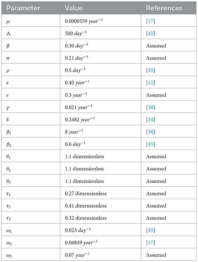
Table 3. Parameter values for numerical simulations.

4.1. Analysis of sensitivity

Definition: The syphilis and COVID-19 co-infection model (3) normalized forward sensitivity index for its variable reproduction number is denoted by ${{R}}_0^{cs}$ its derivative depends on a parameter ζ is defined by SEI$(p)={\frac{\partial {{R}}_0^{cs}}{\partial \zeta }}^{*}\frac{\zeta }{{{R}}_0^{cs}}$ [20, 21, 42].

The syphilis and COVID-19 co-infection model sensitivity index values justify the significance of different parameters in the single infections and co-infection spreading in the community. The parameter which has the highest magnitude of the sensitivity index value compared to other parameter index values is the most sensitive. Here, we have calculated the sensitivity index values in terms of the basic reproduction number ${{R}}_0^{cs}=max\left\{{{R}}_0^s,{{R}}_0^c\right\}$. Using parameter values stated in Table 3, the sensitivity index values of the model (3) are calculated in Tables 4, 5.

TABLE 4

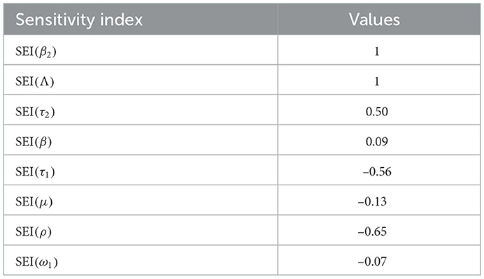
Table 4. Sensitivity indexes of ${{R}}_0^{cs}={{R}}_0^c$.

TABLE 5

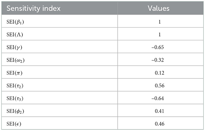
Table 5. Sensitivity indexes of ${{R}}_0^{cs}={{R}}_0^s$.

Using parameter values in Table 3, we have computed ${\Re }_0^{cs}=max\left\{{\Re }_0^c,{\Re }_0^s\right\}=max\left\{2.7,3.2\right\}=3.2$ and biologically, it means that syphilis infection, COVID-19 infection, and their co-infection are spreading in the population. The sensitivity index values stated in Table 4 explain that the recruitment rate Λ and the COVID-19 spreading rate β₂ have a high direct impact on the COVID-19 basic reproduction ${\Re }_0^c$. That means the recruitment rate and the COVID-19 transmission rates are the most sensitive parameters where stakeholders can control the transmission rate by applying prevention and control measures. Similarly, the COVID-19 protection portion τ₁ and the quarantine with treatment rate ρ also have an indirect impact on the COVID-19 reproduction number ${\Re }_0^c$.

Sensitivity indices stated in Table 5 explain that the recruitment rate Λ and syphilis spreading rate β₁ have a high direct impact on the syphilis basic reproduction ${\Re }_0^s$. That means the recruitment rate and syphilis transmission rates are the most sensitive parameters where stakeholders can control the transmission rate by applying prevention and control measures. Similarly, the syphilis protection portion τ₃ and syphilis treatment rate γ have a high indirect effect on the syphilis reproduction number${\Re }_0^s$.

4.2. Results of numerical simulations

4.2.1. Behaviors of solutions of model (3) whenever ${\Re }_0^{\text{c}\text{s}}<1$

In the numerical simulation given in Figure 2, we observed that all the COVID-19 and syphilis co-infection model (3) solutions converge toward the disease-free equilibrium point whenever ${\Re }_0^c=0.71$ and ${\Re }_0^s=0.34$ with β₁ = 0.3 and β₂ = 0.08, respectively. At the co-infection disease-free equilibrium point, each solution curve of the model converges to zero while the susceptible group increases and then becomes constant, implying that the disease-free equilibrium point of the COVID-19 and syphilis co-infection model has global asymptotic stability if ${\Re }_0^{cs}<1.$ Biologically it means the COVID-19 and syphilis co-infection diseases have been eradicated from the community through time whenever ${\Re }_0^{cs}=max\left\{{\Re }_0^c,{\Re }_0^s\right\}=0.71<1$.

FIGURE 2

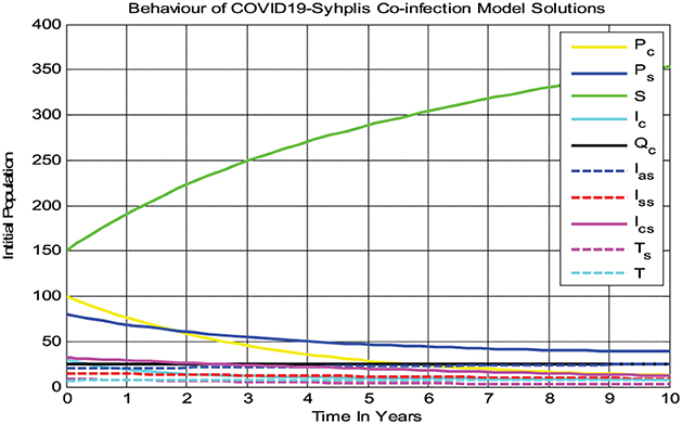
Figure 2. The complete model solutions behavior if ${\Re }_0^{cs}<1$ at β₁ = 0.3 and β₂ = 0.08.

4.2.2. Behaviors of the model solutions whenever ${\Re }_0^{\text{c}\text{s}}>1$

Figure 3 shows that all the COVID-19 and syphilis co-infection model (3) solutions converge toward the endemic equilibrium point whenever ${\Re }_0^c=3.2$ and ${\Re }_0^s=2.1$ with β₁ = 8 and β₂ = 11, respectively. After 10 years, the full-model solutions converge to the endemic equilibrium, while the susceptible population decreases and then remains constant means the COVID-19 and syphilis co-infection model endemic equilibrium point has local asymptotic stability if ${\Re }_0^{cs}=max\left\{{\Re }_0^c,{\Re }_0^s\right\}=3.2>1.$ Biologically, it means that COVID-19 and syphilis co-infection disease spreads throughout the community under consideration.

FIGURE 3

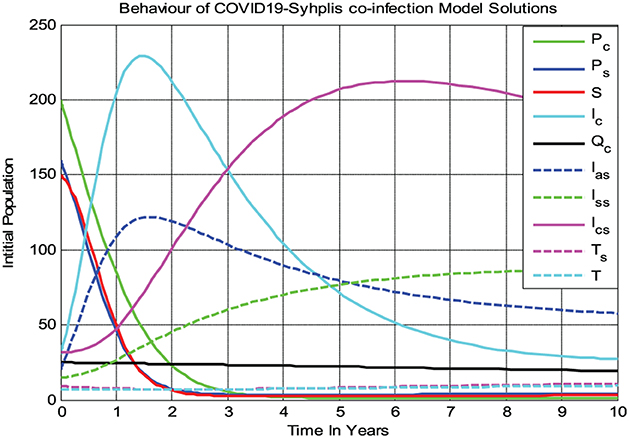
Figure 3. Behaviors of the full model solutions whenever ${\Re }_0^{cs}>1$ at β₁ = 8 and β₂ = 11.

4.2.3. Effects of protection measures on reproduction numbers

The numerical simulation represented by Figure 4 shows that when we maximize the COVID-19 rate of protection τ₁, the reproduction number ${\Re }_0^c$ decreases, implying that the COVID-19 spreading rate decreases. Its biological meaning is that whenever the COVID-19 rate of protection τ₁ > 0.7 the reproduction number ${\Re }_0^c<1$, that is, the COVID-19 infection will be eradicated throughout the community.

FIGURE 4

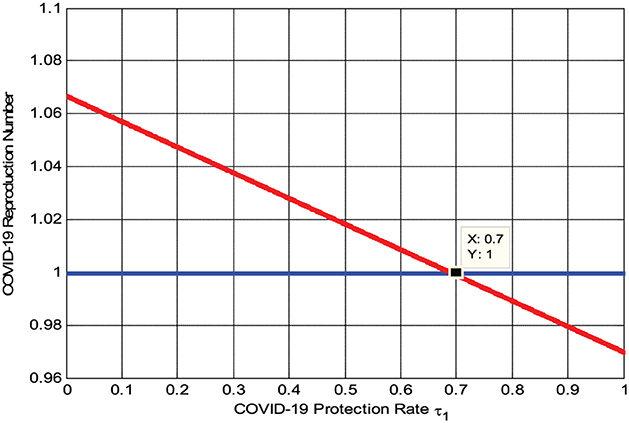
Figure 4. Effect of COVID-19 protection rate on ${\Re }_0^c$.

Here, the numerical simulation represented by Figure 5 shows that whenever we maximize the syphilis protection rate τ₃, the syphilis reproduction number ${\Re }_0^s$ decreases, implying that the syphilis spreading rate decreases. Whenever τ₃ > 0.686 then ${\Re }_0^s<1$, biologically, it means the syphilis infection eradicate from the community.

FIGURE 5

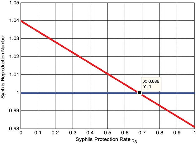
Figure 5. Effect of syphilis protection rate τ₃ on ${\Re }_0^s$.

4.2.4. Impact of treatment on co-infected population

The numerical simulation given in Figure 6 shows that whenever the combined treatment rate ε of the COVID-19 virus and syphilis microorganism Treponema pallidum bacterium co-infected individuals I_cs increases, the number of co-infected individuals decreases; that is, whenever the value of ε increases from 0.3 to 0.8, then the co-infected group I_cs going down.

FIGURE 6

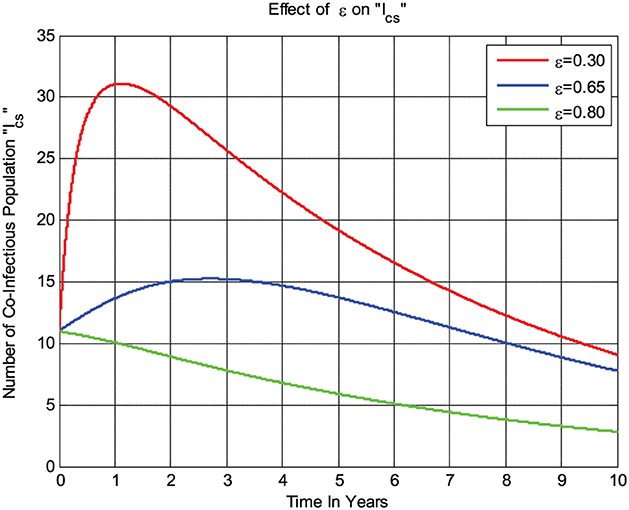
Figure 6. Impact of treatment rate ε on I_cs.

The numerical simulation given in Figure 7 shows that if the treatment rate ρ of COVID-19 increases, then the number of infections in the population decreases; that is, whenever ρ value increases from 0.2 to 0.8 then the infected group I_c decreases.

FIGURE 7

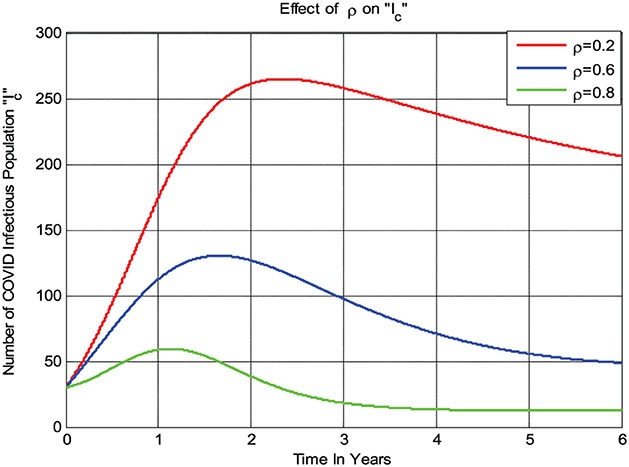
Figure 7. Impact of treatment rate ρ on I_c.

5. Discussions and conclusion

In this study, we have formulated and analyzed a new deterministic mathematical model for gaining insight into the effects of protections and treatments on the transmission dynamics of COVID-19 and syphilis co-infection. Both the positivity and boundedness of the complete model solutions have been discussed to show that the model is both mathematically and biologically meaningful. COVID-19 infection-free equilibrium point, COVID-19 incidence equilibrium point, and local and global stabilities of COVID-19 infection-free and COVID-19 incidence equilibrium points have been examined. Syphilis infection-free equilibrium point, syphilis incidence equilibrium point, and local and global stabilities of syphilis-free and syphilis incidence equilibrium points have been carried out. Using data stated in Table 3, we have carried out and discussed both sensitivity and numerical analyses of the full COVID-19 and syphilis co-infection model. From the analytical and numerical results, we observed that the model disease-free equilibrium points have global asymptotic stability when the basic reproduction numbers are less than unity. Biologically, this means that diseases die out in the community, with the full-model solutions converging to their endemic equilibrium point whenever their basic reproduction number is greater than unity, the reproduction numbers of both the COVID-19 infection and syphilis infection sub-models decreasing when the corresponding protection and treatment rates are maximized, and the numbers of co-infected individuals decreasing when the co-infection treatment rate is increased.

Based on the findings of this study, we recommend public health stakeholders concentrate on increasing both the COVID-19 and syphilis protection rates, as well as the syphilis treatment rate, the COVID-19 isolation with treatment rate, and the co-infection treatment rate, in order to reduce and possibly eradicate syphilis and COVID-19 co-infection transmission in the community. Finally, since no other COVID-19 and syphilis mathematical modeling approach literature has been formulated and analyzed, this study is not exhaustive. Interested researchers can extend this study in different manners, such as including syphilis mother-to-child transmission, COVID-19 vaccination as a new compartment, two-strain COVID-19 co-infection with syphilis, age structure for both infections, the four infection stages of syphilis (primary, secondary, latent, and tertiary), optimal control approach, stochastic method, fractional order method, and applying appropriate real population data.

Data availability statement

All relevant data is contained within the article: The original contributions presented in the study are included in the article/supplementary material, further inquiries can be directed to the corresponding author/s.

Ethics statement

Ethical review and approval was not required for the study on human participants in accordance with the local legislation and institutional requirements. The patients/participants provided their written informed consent to participate in this study.

Author contributions

Both authors listed have made a substantial, direct, and intellectual contribution to the work and approved it for publication.

Acknowledgments

The authors thank Mr. Sitotaw Eshete for his great Wi-Fi contribution that we have used in the study.

Conflict of interest

The authors declare that the research was conducted in the absence of any commercial or financial relationships that could be construed as a potential conflict of interest.

Publisher's note

All claims expressed in this article are solely those of the authors and do not necessarily represent those of their affiliated organizations, or those of the publisher, the editors and the reviewers. Any product that may be evaluated in this article, or claim that may be made by its manufacturer, is not guaranteed or endorsed by the publisher.

References

1. Panovska-Griffiths J. Can mathematical modelling solve the current COVID-19 crisis? BMC Public Health. (2020) 20:1–3. doi: 10.1186/s12889-020-08671-z

PubMed Abstract | CrossRef Full Text | Google Scholar

2. Adiga A, Dubhashi D, Lewis B, Marathe M, Venkatramanan S, Vullikanti A. Mathematical models for COVID-19 pandemic: a comparative analysis. J Indian Inst Sci. (2020) 100:793–807. doi: 10.1007/s41745-020-00200-6

PubMed Abstract | CrossRef Full Text | Google Scholar

3. Musuuza JS, Watson L, Parmasad V, Putman-Buehler N, Christensen L, Safdar N. Prevalence and outcomes of co-infection and superinfection with SARS-CoV-2 and other pathogens: a systematic review and meta-analysis. PLoS ONE. (2021) 16:e0251170. doi: 10.1371/journal.pone.0251170

PubMed Abstract | CrossRef Full Text | Google Scholar

4. Kumar P, Erturk VS, Murillo-Arcila M. A new fractional mathematical modelling of COVID-19 with the availability of vaccine. Results Phys. (2021) 24:104213. doi: 10.1016/j.rinp.2021.104213

PubMed Abstract | CrossRef Full Text | Google Scholar

5. Omame A, Sene N, Nometa I, Nwakanma CI, Nwafor EU, Iheonu NO, et al. Analysis of COVID-19 and comorbidity co-infection model with optimal control. Optimal Control Appl Methods. (2021) 42:1568–90. doi: 10.1002/oca.2748

PubMed Abstract | CrossRef Full Text | Google Scholar

6. Tuite AR, Fisman DN, Greer AL. Mathematical modelling of COVID-19 transmission and mitigation strategies in the population of Ontario, Canada. CMAJ. (2020) 192:E497–505. doi: 10.1503/cmaj.200476

PubMed Abstract | CrossRef Full Text | Google Scholar

7. Boukanjime B, Caraballo T, El Fatini M, El Khalifi M. Dynamics of a stochastic coronavirus (COVID-19) epidemic model with Markovian switching. Chaos Solitons Fractals. (2020) 141:110361. doi: 10.1016/j.chaos.2020.110361

PubMed Abstract | CrossRef Full Text | Google Scholar

8. Din A, Khan A, Baleanu D. Stationary distribution and extinction of stochastic coronavirus (COVID-19) epidemic model. Chaos Solitons Fractals. (2020) 139:110036. doi: 10.1016/j.chaos.2020.110036

PubMed Abstract | CrossRef Full Text | Google Scholar

9. Abdela SG, Berhanu AB, Ferede LM, van Griensven J. Essential healthcare services in the face of COVID-19 prevention: experiences from a referral hospital in Ethiopia. Am J Trop Med Hyg. (2020) 103:1198. doi: 10.4269/ajtmh.20-0464

PubMed Abstract | CrossRef Full Text | Google Scholar

10. Gumel AB, Lubuma J, Sharomi O, Terefe YA. Mathematics of a sex-structured model for syphilis transmission dynamics. Math Methods Appl Sci. (2018) 41:8488–513. doi: 10.1002/mma.4734

PubMed Abstract | CrossRef Full Text | Google Scholar

11. Momoh AA, Bala Y, Washachi DJ, Déthié D. Mathematical analysis and optimal control interventions for sex structured syphilis model with three stages of infection and loss of immunity. Adv Diff Equ. (2021) 2021:1–26. doi: 10.1186/s13662-021-03432-7

PubMed Abstract | CrossRef Full Text | Google Scholar

12. Peeling RW, Mabey D, Kamb ML, Chen XS, Radolf JD. “Benzaken.” AS Syphilis. Nat Rev Dis Prim. (2017) 3:17073. doi: 10.1038/nrdp.2017.73

PubMed Abstract | CrossRef Full Text

13. Peeling RW, Hook III EW. The pathogenesis of syphilis: the Great Mimicker, revisited. J Pathol. (2006) 208:224–32. doi: 10.1002/path.1903

PubMed Abstract | CrossRef Full Text | Google Scholar

14. Saad-Roy CM, Shuai Z, Van den Driessche P. A mathematical model of syphilis transmission in an MSM population. Math Biosci. (2016) 277:59–70. doi: 10.1016/j.mbs.2016.03.017

PubMed Abstract | CrossRef Full Text | Google Scholar

15. Tessema B, Yismaw G, Kassu A, Amsalu A, Mulu A, Emmrich F, et al. Seroprevalence of HIV, HBV, HCV and syphilis infections among blood donors at Gondar University Teaching Hospital, Northwest Ethiopia: declining trends over a period of five years. BMC Infect Dis. (2010) 10:1–7. doi: 10.1186/1471-2334-10-111

PubMed Abstract | CrossRef Full Text | Google Scholar

16. World Health Organization. WHO Guidelines for the Treatment of Treponema pallidum (Syphilis). Geneva: WHO (2016).

Google Scholar

17. Iboi E, Okuonghae D. Population dynamics of a mathematical model for syphilis. Appl Math Model. (2016) 40:3573–90. doi: 10.1016/j.apm.2015.09.090

CrossRef Full Text | Google Scholar

18. Milner FA, Zhao R. A new mathematical model of syphilis. Math Model Nat Phenom. (2010) 5:96–108. doi: 10.1051/mmnp/20105605

CrossRef Full Text | Google Scholar

19. Tuite AR, Fisman DN, Mishra S. Screen more or screen more often? Using mathematical models to inform syphilis control strategies. BMC Public Health. (2013) 13:1–9. doi: 10.1186/1471-2458-13-606

PubMed Abstract | CrossRef Full Text | Google Scholar

20. Teklu SW, Rao KP. HIV/AIDS-Pneumonia codynamics model analysis with vaccination and treatment. Comput Math Methods Med. (2022) 2022:3105734. doi: 10.1155/2022/3105734

PubMed Abstract | CrossRef Full Text | Google Scholar

21. Teklu SW, Mekonnen TT. HIV/AIDS-pneumonia coinfection model with treatment at each infection stage: mathematical analysis and numerical simulation. J Appl Math. (2021) 2021:5444605. doi: 10.1155/2021/5444605

PubMed Abstract | CrossRef Full Text | Google Scholar

22. Danane J, Allali K, Hammouch Z, Nisar KS. Mathematical analysis and simulation of a stochastic COVID-19 Lévy jump model with isolation strategy. Results Phys. (2021) 23:103994. doi: 10.1016/j.rinp.2021.103994

PubMed Abstract | CrossRef Full Text | Google Scholar

23. Bonyah E, Chukwu CW, Juga ML. Modeling fractional order dynamics of syphilis via Mittag-Leffler law. medRxiv. (2021). doi: 10.3934/math.2021485

CrossRef Full Text | Google Scholar

24. Nabi KN, Abboubakar H, Kumar P. Forecasting of COVID-19 pandemic: from integer derivatives to fractional derivatives. Chaos Solitons Fractals. (2020) 141:110283. doi: 10.1016/j.chaos.2020.110283

PubMed Abstract | CrossRef Full Text | Google Scholar

25. Nabi KN, Kumar P, Erturk VS. Projections and fractional dynamics of COVID-19 with optimal control strategies. Chaos Solitons Fractals. (2021) 145:110689. doi: 10.1016/j.chaos.2021.110689

PubMed Abstract | CrossRef Full Text | Google Scholar

26. Kumar P, Erturk VS, Murillo-Arcila M, Banerjee R, Manickam A. A case study of 2019-nCOV cases in Argentina with the real data based on daily cases from March 03, 2020 to March 29, 2021 using classical and fractional derivatives. Adv Diff Equ. (2021) 2021:1–21. doi: 10.1186/s13662-021-03499-2

PubMed Abstract | CrossRef Full Text | Google Scholar

27. Etemad S, Avci I, Kumar P, Baleanu D, Rezapour S. Some novel mathematical analysis on the fractal-fractional model of the AH1N1/09 virus and its generalized Caputo-type version. Chaos Solitons Fractals. (2022) 162:112511. doi: 10.1016/j.chaos.2022.112511

CrossRef Full Text | Google Scholar

28. Zarin R, Khan A, Kumar P. Fractional-order dynamics of Chagas-HIV epidemic model with different fractional operators. AIMS Math. (2022) 7:18897–924. doi: 10.3934/math.20221041

CrossRef Full Text | Google Scholar

29. Gao W, Veeresha P, Baskonus HM, Prakasha DG, Kumar P. A new study of unreported cases of 2019-nCOV epidemic outbreaks. Chaos Solitons Fractals. (2020) 138:109929. doi: 10.1016/j.chaos.2020.109929

PubMed Abstract | CrossRef Full Text | Google Scholar

30. Kumar P, Erturk VS, Abboubakar H, Nisar KS. Prediction studies of the epidemic peak of coronavirus disease in Brazil via new generalised Caputo type fractional derivatives. Alexandr Eng J. (2021) 60:3189–204. doi: 10.1016/j.aej.2021.01.032

CrossRef Full Text | Google Scholar

31. Vellappandi M, Kumar P, Govindaraj V. Role of fractional derivatives in the mathematical modeling of the transmission of Chlamydia in the United States from 1989 to 2019. Nonlinear Dyn. (2022) 2022:1–15. doi: 10.1007/s11071-022-08073-3

PubMed Abstract | CrossRef Full Text | Google Scholar

32. Abbas S, Tyagi S, Kumar P, Ertürk VS, Momani S. Stability and bifurcation analysis of a fractional-order model of cell-to-cell spread of HIV-1 with a discrete time delay. Math Methods Appl Sci. (2022) 45:7081–95. doi: 10.1002/mma.8226

CrossRef Full Text | Google Scholar

33. Teklu SW, Terefe BB. Mathematical modeling analysis on the dynamics of university students animosity towards mathematics with optimal control theory. Sci Rep. (2022) 12:1–19. doi: 10.1038/s41598-022-15376-3

PubMed Abstract | CrossRef Full Text | Google Scholar

34. Babaei A, Ahmadi M, Jafari H, Liya A. A mathematical model to examine the effect of quarantine on the spread of coronavirus. Chaos Solitons Fractals. (2021) 142:110418. doi: 10.1016/j.chaos.2020.110418

PubMed Abstract | CrossRef Full Text | Google Scholar

35. Basnarkov L. SEAIR. Epidemic spreading model of COVID-19. Chaos Solitons Fractals. (2021) 142:110394.

PubMed Abstract | Google Scholar

36. Mohamadou Y, Halidou A, Kapen PT. A review of mathematical modeling, artificial intelligence and datasets used in the study, prediction and management of COVID-19. Appl Intell. (2020) 50:3913–25. doi: 10.1007/s10489-020-01770-9

PubMed Abstract | CrossRef Full Text | Google Scholar

37. Ndaïrou F, Area I, Nieto JJ, Torres DF. Mathematical modeling of COVID-19 transmission dynamics with a case study of Wuhan. Chaos Solitons Fractals. (2020) 135:109846. doi: 10.1016/j.chaos.2020.109846

PubMed Abstract | CrossRef Full Text | Google Scholar

38. Nwankwo A, Okuonghae D. Mathematical analysis of the transmission dynamics of HIV syphilis co-infection in the presence of treatment for syphilis. Bull Math Biol. (2018) 80:437–92. doi: 10.1007/s11538-017-0384-0

PubMed Abstract | CrossRef Full Text | Google Scholar

39. Teklu SW, Kotola BS. The impact of protection measures and treatment on pneumonia infection: a mathematical model analysis supported by numerical simulation. bioRxiv. (2022). doi: 10.1101/2022.02.21.481255

CrossRef Full Text | Google Scholar

40. Vellappandi M, Kumar P, Govindaraj V. Role of vaccination, the release of competitor snails, chlorination of water, and treatment controls on the transmission of bovine schistosomiasis disease: a mathematical study. Phys Script. (2022) 97:074006. doi: 10.1088/1402-4896/ac7421

CrossRef Full Text | Google Scholar

41. Oshinubi K, Buhamra SS, Al-Kandari NM, Waku J, Rachdi M, Demongeot J. Age dependent epidemic modeling of COVID-19 outbreak in Kuwait, France, and Cameroon. In: Send P, editor. Healthcare (Vol. 10, No. 3). MDPI (2022), p. 482.

PubMed Abstract | Google Scholar

42. Teklu SW. Mathematical analysis of the transmission dynamics of COVID-19 infection in the presence of intervention strategies. J Biol Dyn. (2022) 16:640–64. doi: 10.1080/17513758.2022.2111469

PubMed Abstract | CrossRef Full Text | Google Scholar

43. Castillo-Chavez C, Feng Z, Huang W. On the computation of ro and its role on. In: Castillo-Chavez PC, Blower S, Driessche P, Kirschner D, Yakubu A-A, editors. Mathematical Approaches for Emerging and Reemerging Infectious Diseases: An Introduction. vol 1, 229 (2002). doi: 10.1007/978-1-4757-3667-0_13

CrossRef Full Text | Google Scholar

44. Van den Driessche P, Watmough J. Reproduction numbers and sub-threshold endemic equilibria for compartmental models of disease transmission. Math Biosci. (2002) 180:29–48. doi: 10.1016/S0025-5564(02)00108-6

PubMed Abstract | CrossRef Full Text | Google Scholar

45. Mekonen KG, Balcha SF, Obsu LL, Hassen A. Mathematical modeling and analysis of TB and COVID-19 coinfection. J Appl Math. (2022) 2022:1–20. doi: 10.1155/2022/2449710

CrossRef Full Text | Google Scholar