Rank–Polyserial Correlation: A Quest for a “Missing” Coefficient of Correlation

Introduction

Over the years, scholars have developed many estimators of the association of two variables X and Y, depending on their scale properties. Usually, these are based either on the covariance between X and Y (e.g., Pearson's tetrachoric, biserial, polyserial, point-biserial, point-polyserial, or polychoric correlation) or the ratio of the favourable combinations and all combinations (e.g., Cureton's rank-biserial correlation, Goodman–Kruskal tau, lambda, gamma, Kendall's tau family, Pearson's eta and phi, or Somers' delta). These coefficients are divided into coefficients of observed and inferred association (see [1]). The observed association is estimated for the manifested variables and the inferred association for the latent variables or for the combination of an observed and a latent variable (see Figure 1). This difference between the latent and observed variables is discussed first, after which the factual estimators are discussed.

FIGURE 1

Figure 1. Two latent variables η and ξ manifested as X and g with ordinal or interval scales.

Statistical Model Latent to Correlations

Assume two continuous variables ξ and η with the unknown joint distribution. For the later use of variables with different scales related to the proposed rank–polyserial coefficients of correlation, let these latent variables be manifested as two observed variables g with a narrower scale and X with a wider scale with x_i = 1, …, r with distinctive ordinal categories and X with y_i = 1, …, c distinctive categories with metric properties (ordinal, interval, pseudo-continuous¹ or continuous scales), respectively, and r < < c. The variable g is related to ξ and X to η with the class limits or thresholds γ_i and τ_j so that

$\begin{array}{ll}g=x_{\text{i}},\text{if }{\gamma }_{i-1}\le \xi <{\gamma }_i,i=1,2,\dots ,r& (\mathrm{1a})\end{array}$

and

$\begin{array}{ll}X=y_j,\text{if }{\tau }_{j-1}\le \eta <{\tau }_j,j=1,2,\dots ,c& (\mathrm{1b})\end{array}$

For the observed values, x₁ < x₂ < ... < x_r−1 and y₁ < y₂ < ... < y_r−1, and for convenience, γ₀ = τ₀ = −∞ and γ_r = τ_c = +∞. The relation of the variables with related symbols is illustrated in Figure 1 where n_gX denotes the number of times the observation (g, X) is obtained in the sample, and the latent variables are assumed to be normally distributed.

In the measurement modelling settings used in the numerical examples, an item g and a score variable X compiled by a set of test items share the common latent variable θ, such as achievement in mathematics, which is manifested in two variables, item g and the test score X. As above, the threshold values of θ for each category in g and X are denoted by γ_i and, respectively. Hence, g with r = 1, …, r distinctive ordinal categories and score variable X with c = 1, …, c distinctive categories with a metric scale are related to θ so that g = x_i, if γ_i−1 ≤ θ < γ_i, i = 1, 2, …, r and X = y_j, if τ_j−1 ≤ θ < τ_j, j = 1, 2, …, c, and γ₀ = τ₀ = −∞ and γ_R = τ_C = +∞. Often, the scoring starts from zero, which is illustrated in Figure 2. Then, the degrees of freedom are df (g) = r – 1 and df (X) = c – 1.

FIGURE 2

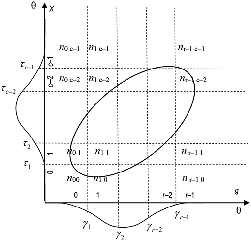
Figure 2. One latent variable θ manifested in two different scales.

Multitudes of Coefficients of Association

The estimators of the association are really many. Olsson et al. [1] collected some estimators as a typology, and their work is elaborated and rethought in what follows (see Table 1).

TABLE 1

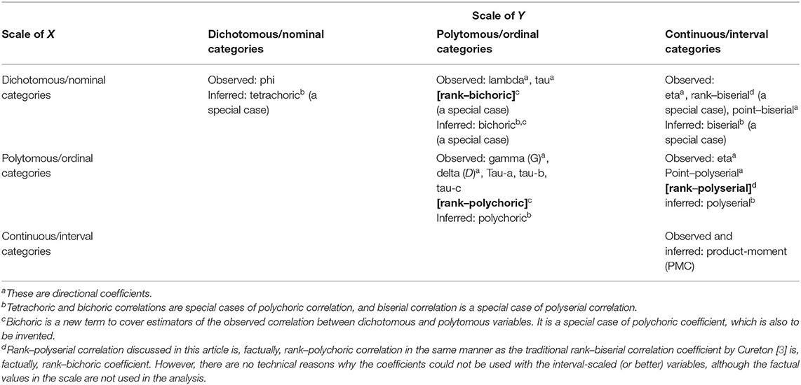
Table 1. Coefficients of association by the scale properties of the observed variables X and Y.

At the beginning of the twentieth Century, Karl Pearson initiated and developed many coefficients for the observed association that still are in our use. The mechanics of the product-moment correlation coefficient between two observed variables with a metric scale (PMC; Pearson [4] onwards based on Bravais [5]) is used in the point–biserial correlation (R_PB = ρ_gX) between an observed dichotomized or binary g and a metric-scaled X and in point–polyserial correlation (R_PP = ρ_gX) between a polytomous ordinal g and a metric-scaled X. These are classic estimators of the item–score association in the measurement modelling settings.

Pearson also presented coefficient phi [6] suitable for two observed nominal-scaled variables, and coefficient eta [7, 8] suitable for an observed nominal- or ordinal-scaled variable and a metric variable. Later, such robust, non-parametric coefficients were developed for the observed association for ordinal-scaled variables as Goodman's and Kruskal's lambda, tau, and gamma (G) [9, 10], the family of Kendall's Tau ([11] onwards) and the family of Somers' D [12], including Cureton's rank-biserial correlation (R_RB) [3, 13, 14]; R_RB is a special case of D in the case of a binary variable g and ordinal-scaled X (see Newson [15]). This relationship is deepened later.

For the coefficients for inferred association between the latent variables ξ and η, the most known is the polychoric correlation (R_PC = ρ_ξη) and its special case, tetrachoric correlation suitable for two latent, dichotomized variables (R_TC = ρ_ξη) [16, 17]. Pearson also initiated polyserial correlation (R_PS = ρ_ξX) between a latent variable related to the variable with a shorter scale (ξ) and observed X, and its special case, the biserial correlation for the dichotomized ξ and observed X (R_BS) [17, 18]. Common to all these is that we intend to infer what could the correlation between the variables be if measured in their latent, unobservable form.

When it comes to the factual estimation of the inferred association of two observed ordinal or interval-scaled variables with (theoretical, unobservable) latent variables, we have established routines for estimating R_PC (e.g., [19–21]; see also [22]), as well as R_BS and R_PS (see [23]). The traditional routines of calculating the estimates by R_BS and R_PS led, however, to practicalities that the estimates reached out of range values (R_BS, R_PS>> +1) if the embedded PMC and the item variance are high to start with (e.g., [24]; see the discussion in, e.g., [25, 26]; see the computational form in Eq. 34). One of the best alternatives for R_BS and R_PS, if not the best, is a coefficient called r-bireg and r-polyreg correlation (R_REG; see [27, 28]; see Eq. 37), which have behaved quite optimally in simulations (see, e.g., [29]).

Missing Coefficients of Correlation

As highlighted in Table 1, we seem to miss a set of coefficients for the ordinal variables: rank–polyserial and rank–polychoric correlation coefficients (R_RP) for the observed association between the ordinal-scaled or metric variables. In the ERIC database with more than 1.2 million articles and research papers, we found no hits with the fixed keywords “rank polyserial” or “rank polychoric” at the time of finalising the article (April 2022). Nevertheless, some possible options such as R_RP are available. These are discussed in this article.

Research Questions

This article discusses and studies the characteristics of a set of coefficients of correlation that could be called either rank polyserial or rank polychoric correlation coefficient. In what follows, the name rank–polyserial is preferred because of its connection to rank–biserial (R_RB) correlation by Cureton. Although the options for R_RP discussed here are not restricted to item analysis settings, their characteristics are studied in the framework of measurement modelling. After all, estimators of the association have a central role to play, for example, as the estimators of the item–score association and embedded to estimators of reliability (see discussion in, e.g., [26, 29, 30]). This perspective leads us to compare the options of R_RP with its traditional alternatives: R_PP = ρ_gX, often called item–total correlation (Rit), Henrysson's corrected item–total correlation (R_PPH) [31], also known as item–rest correlation (Rir), coefficient eta directed so that X explains the order in g or “g given X”², that is, η(g|X), as well as polyserial and polychoric coefficients of correlation (R_PS, R_PC).

After introducing a set of possible coefficients relevant to be taken as R_RP, the following questions are asked:

1) What are the statistical properties of the new coefficients?

2) What are the general characteristics of the new coefficient in comparison with other classical estimators of association?

Empirical notes of the comparison are given based, first, on a simple numeric example, to introduce the manual computation; second, on a larger dataset with 6,932 items from 1,440 tests from real-world testing settings to study the performance of the estimators in real-life settings; and third, a simulation dataset of 22,842 estimates related to a hypothetic design there two identical items are truncated into two different forms to study their tendency to give deflated estimates. Characteristics of the dataset are discussed later with numerical examples.

Options for Rank–Polyserial and Rank–Polychoric Coefficients of Correlation and a Measurement Model for Assessing the Possible Deflation in the Estimates

In what follows, first, rank–biserial correlation is discussed. In Rank–Biserial Correlation and U-Test Statistic Section, Cureton's ρ_RB is shown to be strictly related to the directed Mann–Whitney U-test statistic ([40]; see [14, 41]), and, hence, second, this connection is utilised when deriving a new coefficient of correlation, rank–polyserial correlation in Rank–Polyserial Correlation and JT-Test Statistic section. Third, another possible coefficient of rank–polyserial coefficients is introduced in Identity of JT_gX and Somers D, Relation of JT_gX and Goodman–Kruskal G, and Dimension-Corrected G and D as Options for the Coefficient of Rank–Polyserial Correlation sections where their connexion to Jonckheere–Terpstra test statistic is shown. Numerical examples of computing the estimators are given later.

Rank–Biserial Correlation and U-Test Statistic

Assume two sub-samples i = 0 and j = 1 where i and j could be males and females or incorrect and correct answers in a test item. The standard procedure of the U-test produces two statistics, where U₁ refers to the higher values and U₂ refers to the lower values (see the estimation of U-test in, e.g., [33, 37]). Wendt's [14] modification of ρ_RB is

$\begin{array}{ll}{R}_{RB}=1-\frac{2U}{n_0{n}_1}& (2)\end{array}$

related to the lower of the groups i, j regardless of the statistics U₁ and U₂; this is discussed later.

The original idea by Cureton was based on the proportion of favourable cases (f) and unfavourable cases (u)

$\begin{array}{ll}{R}_{RB}=f-u=f-(1-f)=2f-1,& (3)\end{array}$

and this idea is used later in deriving the corresponding rank–polyserial correlation. To compute the proportion of favourable cases, the mechanics and heuristics of U-test statistics could be used. The heuristic of the observed U statistic is to compute the number of “favourable” incidents of how many observations from the subsample i = 0 fall below each observation from the subsample j = 1 after the variable of interest g is ordered by a metric variable X. If no tied pairs are obtained, the observed U statistic related to the sub-population j = 1 ($U_{gX}^{obs}$) is the sum of those sums (see, e.g., [33, 37]). With tied cases, Wilcoxon's method [42] produces the correct value; this is discussed later. The maximal value of the U statistic is reached when all cases in the subsample i = 0 (altogether, n₀ cases) are ranked lower than all cases in subsample j = 1 (altogether, n₁ cases):

$\begin{array}{ll}{U}_{gX}^{Max}=n_0{n}_1& (4)\end{array}$

In the binary (ordinal) case, the proportion of “favourable” cases is the ratio of the observed and maximal U statistic $U_{gX}^{Obs}/U_{gX}^{Max}$that varies between 0 and 1. This ratio is rescaled by multiplying it with 2 and relocated by −1, and we get the values ranging from −1 to +1 as is standard in coefficients of correlation:

$\begin{array}{ll}{R}_{RB}=2\times \frac{U_{gX}^{Obs}}{U_{gX}^{Max}}-1=2\times \frac{U_{gX}^{Obs}}{n_0{n}_1}-1& (5)\end{array}$

Notably, Eq. (5) is identical to Eq. (1), while Wendt's formula (Eq. 2) is based on the subsample i = 0, and Eq. (5) is based on the subsample j = 1. All in all, R_RB is the rescaled and relocated proportion of logically (ascending) located cases within the categorical (ordinal) variable g after they are ordered by the metric variable X. Notably, Eq. (5) strictly corresponds with Cureton's idea (R_RB = 2×f – 1; see Eq. 3). The further the erroneous locations from the deterministic position are and the more these erroneous locations are, the lower the value in the estimate. This is illustrated later with a numerical example.

Rank–Polyserial Correlation and JT-Test Statistic

Jonckheere–Terpstra test statistic (JT) [43, 44], also known as Jonckheere trend test [43], with a directional nature generalises U-test statistic and its heuristic to polytomous ordinal cases (see [33, 37]). This connection is used in proposing a new estimator of correlation, carrying characteristics relevant to R_RP.

Assume an ordinal variable g with observed categories r = i, j, and i < j and the metric variable X. Then, n_i and n_j are the numbers of cases in the subsamples i and j in variable g. In the 5-point Likert scale, as an example, one pair of subsamples is i = 1 and j = 4. In general, we have r(r − 1)/2 possible values for the $U_{gXij}^{Obs}$ statistics. In the case of the 5-point Likert scale, as an example, we obtain 5 × 4/2 = 10 values: U₁₂, U₁₃, U₁₄, U₁₅, U₂₃, U₂₄, U₂₅, U₃₄, U₃₅, and U₄₅. In the computational procedure in what follows, the sum of the ranks in the higher of the subsamples i, j, $W_j={\displaystyle \sum _{j=1}^{n_1}}{R}_j$ is of interest.

In the same manner, as with R_RB, the essence of the new coefficient is the ratio of the observed and maximal JT statistics ($J{T}_{gX}^{Obs}$ and $J{T}_{gX}^{Max}$, respectively). $J{T}_{gX}^{Obs}$ can be expressed by using the U statistic:

$\begin{array}{ll}J{T}_{gX}^{Obs}={\displaystyle \sum _{i<j}^r}{U}_{gXij}^{Obs}& (6)\end{array}$

(see [33, 37]) where $U_{gXij}^{Obs}$ refers to the observed U statistics related to all the pairs of subsamples i and j. This statistic indicates the number of “favourable” incidents where, after ordering by X, the cases with a higher value in X have a higher value also in g. The observed U statistic for the observed JT statistic can be computed by using Wilcoxon's W statistic [42]:

$\begin{array}{ll}{U}_{gX}^{Obs}=W_j-\frac{n_j(n_j+1)}{2}& (7)\end{array}$

where W_j is the sum of the ranks of the higher of the subsamples i and j. The maximal value for each U statistic is reached when all the test-takers in subsample j (altogether, n_j cases) are ranked higher than all test-takers in the subsample i (altogether, n_i cases). Hence, with each pair of subsamples,

$\begin{array}{ll}{U}_{gXij}^{Max}=n_i{n}_j,& (8)\end{array}$

and the maximal value of the observed JT statistic is the sum of these values

$\begin{array}{ll}J{T}_{gX}^{Max}={\displaystyle \sum _{i<j}^r}{U}_{gXij}^{Max}={\displaystyle \sum _{i<j}^r}{n}_i{n}_j& (9)\end{array}$

Because Eqs. (6), (7), (8), and (9), paralleled with the rank–polyserial correlation, a new coefficient rank–polyserial correlation is defined as:

$\begin{array}{l}J{T}_{gX}=R_{RP}=2\times \frac{J{T}_{gX}^{Obs}}{J{T}_{gX}^{Max}}-1=2\times \frac{J{T}_{gX}^{Obs}}{{\displaystyle \sum _{i<j}^r}{n}_i{n}_j}-1\\ =2\times \frac{{\displaystyle \sum _{j=1}^r}\left[W_j-n_j(n_j+1)/2\right]}{{\displaystyle \sum _{i<j}^r}{n}_i{n}_j}-1& (10)\end{array}$

where r refers to the number of categories in the variable with a narrower scale (g), j refers to the higher number of the subsamples i and j in g, and W_j is the sum of the ranks in the higher number of the subsamples i and j.

The core of the coefficient JT_gX is the probability statistics of the ratio of observed and maximal JT statistic $J{T}_{gX}^{Obs}/J{T}_{gX}^{Max}$, that is, the proportion of “favourable” cases in the spirit of Cureton that varies between 0 and 1. This ratio is rescaled by multiplying it by 2 and relocated by −1 to the same scale as the Pearson correlation. This coefficient could be called either rank–polyserial correlation as a legacy to Cureton's rank–biserial correlation or rank–polychoric coefficient as a robust counterpart to the classic polychoric correlation; here, the former is used, but an abbreviation R_RP is used to keep both interpretations open.

The value JT_gX = +1 indicates the positive deterministic pattern in g; after being ordered by X, all the observations in the higher subsample(s) j are ordered higher than those in the lower subsample(s) i. By using the concept of “concordant pairs” familiar from many robust coefficients of association such as Somers D and Goodman–Kruskal G, JT_gX = +1 refers to the situation where all the pairs of observations are concordant. The further the erroneous locations from the deterministic position are and the more these erroneous locations are, the closer is the magnitude in JT_gX to zero. The value JT_gX = 0 refers to a situation where the observations are randomly spread in variable g after being ordered by X. The value JT_gX = −1 indicates the ultimate situation that all the cases in the lower subsample(s) i would be ranked higher than those in the higher subsample(s) j. By using the concept “discordant pairs,” the last refers to the situation in which all the pairs of observations are discordant. The interpretation of the magnitude of the estimates by JT_gX is the same as that in R_PP (ρ_gX), with the note that, in real-life datasets, R_PP cannot reach perfect +1 or −1 (see e.g., [29, 45]) while JT_gX can.

In the specific case that there are only two categories in g, for example, when only two categories are obtained in a Likert type of scale (see later the numerical example) or in a binary case, $U_{gXij}^{Obs}$ includes only one U statistic, U_ij, and $J{T}_{gX}^{Obs}$ is reduced to ordinary U-test statistic related to the higher number of the subsamples i, j. Hence, because of Eqs. (10), (2), (4), (5), in the binary or dichotomous case, R_RB is a special case of JT_gX:

$\begin{array}{ll}J{T}_{gX}=2\times \frac{{\displaystyle \sum _{i<j}^r}{U}_{gXij}^{Obs}}{{\displaystyle \sum _{i<j}^r}{U}_{gXij}^{Max}}-1=2\times \frac{U_{gXij}^{Obs}}{n_i{n}_j}-1=R_{RB}& (11)\end{array}$

Identity of JT_gX and Somers D

JT_gX has the identity of Somers' D directed, so that “g given X,” that is, D(g|X), henceforth, plainly D. Assume two variables, ordinal g with the subsamples i < r with observed values x_i and ordinal X with subsamples with observed values y_j sampled from the same bivariate distribution forming an r × c cross-tabulation. The number of cases in the subsamples related to g is n_i and

$\begin{array}{ll}N={\displaystyle \sum _{i=1}^r}{n}_i& (12)\end{array}$

The computational form of D directed so that “g given X” can be expressed as

$\begin{array}{ll}D\left(g|X\right)=\frac{2(P-Q)}{N^2-{\displaystyle \sum _{i=1}^r}\left({n_i}^2\right)}& (13)\end{array}$

(e.g., [32, 33, 37]) where P is the sum of the concordant pairs of two observations x_i and x_j, and, correspondingly, y_i and y_j, and Q is the sum of the discordant pairs. Because of Eq. (12),

$\begin{array}{ll}{N}^2-{\displaystyle \sum _{i=1}^r}\left({n_i}^2\right)=2{\displaystyle \sum _{i<j}^r}{n}_i{n}_j& (14)\end{array}$

(see [32]). Hence, because of Eqs. (13) and (14), D can be rewritten as

$\begin{array}{ll}D\left(g|X\right)=\frac{2(P-Q)}{2{\displaystyle \sum _{i<j}^r}{n}_i{n}_j}=\frac{P-Q}{{\displaystyle \sum _{i<j}^r}{n}_i{n}_j}& (15)\end{array}$

When all the pairs are concordant, Q equals 0, and

$\begin{array}{ll}D\left(g|X\right)=\frac{P^{Max}}{{\displaystyle \sum _{i<j}^r}{n}_i{n}_j}=1& (16)\end{array}$

and, consequently,

$\begin{array}{ll}{P}^{Max}={\displaystyle \sum _{i<j}^r}{n}_i{n}_j& (17)\end{array}$

The statistic Q is strictly related to P^Max:

$\begin{array}{ll}Q=P^{Max}-P& (18)\end{array}$

Hence, because of Eqs. (17) and (18),

$\begin{array}{ll}Q={\displaystyle \sum _{i<j}^r}{n}_i{n}_j-P,& (19)\end{array}$

and D(g|X) can be rewritten as

$\begin{array}{l}D\left(g|X\right)=\frac{P-Q}{{\displaystyle \sum _{i<j}^r}{n}_i{n}_j}=\frac{P-{\displaystyle \sum _{i<j}^r}{n}_i{n}_j+P}{{\displaystyle \sum _{i<j}^r}{n}_i{n}_j}=\frac{2P-{\displaystyle \sum _{i<j}^r}{n}_i{n}_j}{{\displaystyle \sum _{i<j}^r}{n}_i{n}_j}\\ =2\times \frac{P}{{\displaystyle \sum _{i<j}^r}{n}_i{n}_j}-1& (20)\end{array}$

Notably, from the JT statistic viewpoint, the observed JT statistic is the number of concordant pairs in the positive direction:

$\begin{array}{ll}J{T}_{gX}^{Obs}=P& (21)\end{array}$

Because of Eqs. (10), (21), and (20), JT_gX can be expressed as

$\begin{array}{ll}J{T}_{gX}=2\times \frac{J{T}_{gX}^{Obs}}{{\displaystyle \sum _{i<j}^r}{n}_i{n}_j}-1=2\times \frac{P}{{\displaystyle \sum _{i<j}^r}{n}_i{n}_j}-1=D\left(g|X\right)& (22)\end{array}$

Hence, because both JT_gX(= R_RP) and Cureton's (and Glass' and Wendt's) R_RB is a special case of Somers' D (of the derivation for R_RB, see [15]), these coefficients form a family related to Somers' D(X|Y); see other coefficients and test statistics related to the same family in, e.g., Metsämuuronen [32]. Although JT_gX is a specific case of Somers' D(g|X), the advantage over D in measurement modelling settings is that it leads us strictly to the correct form of the three alternatives produced by the standard procedures of calculating Somers' D.

Because JT_gX has the identity of D, it carries the same advantages and weaknesses as D does. One of the advances is that the sampling variance and asymptotic standard errors of JT_gX are known (see, e.g., [32, 46, 47]; see Supplementary Appendix 1). One of the weaknesses of D is that it tends to underestimate item–score association in an obvious manner when the number of categories exceeds 3 (see [25, 48, 49]). This characteristic is discussed later.

Relation of JT_gX and Goodman–Kruskal G

Although it is not a generally known fact, Goodman–Kruskal gamma (G) is a directional measure in the same direction as D(g|X) (see the proof in [32]), although, usually, G is taken as a symmetric measure (see, e.g., [50]) because it produces only one estimate of correlation. However, if there are no tied pairs in the dataset, as is the case when the metric variable has no tied cases (see other cases in [32]), G equals D(g|X) and not D(X|g) nor D (Symmetric).

Except for the special case of no tied cases, the estimates by G are more liberal than those by D. The main difference between G and D is how they treat the tied pairs. By using the concepts of concordant and discordant pairs (P and Q) as with D, G is computed by

$\begin{array}{ll}G=\frac{2\times (P-Q)}{2\times (P+Q)}=\frac{(P-Q)}{(P+Q)}& (23)\end{array}$

The number of all possible pairs can be expressed as

$\begin{array}{l}{D}_g=N^2-{\displaystyle \sum _{i=1}^r}\left({n_i}^2\right)=2\times \left(P+T_g\right)+2\times \left(Q+T_g\right)\\ =2\times (P+Q)+4T_g& (24)\end{array}$

(see, e.g., [32]) where 4T_g refers to the number of tied pairs, that is, the pairs where the direction is not known, and the magnitude of P, Q, and T_g is thought double-sized than the simplified formulae indicate³. In computing the probability by G, the tied pairs are omitted and, hence, the number of pairs used in the estimation is

$\begin{array}{ll}2\times (P+Q)=\left[N^2-{\displaystyle \sum _{i=1}^r}\left({n_i}^2\right)\right]-4T_g& (25)\end{array}$

Then, because of Eq. (14) and because Eq. (25), $Q={\displaystyle \sum _{l<h}^R}{n}_l{n}_h-\left(P+2T_g\right)$, and

$\begin{array}{l}G=\frac{2\times (P-Q)}{2\times (P+Q)}=\frac{2\times (P-Q)}{\left[N^2-{\displaystyle \sum _{i=1}^r}\left({n_i}^2\right)\right]-4T_g}\\ =\frac{2\times (P-Q)}{2{\displaystyle \sum _{l<h}^r}{n}_l{n}_h-4T_g}=\frac{2\times P}{{\displaystyle \sum _{l<h}^R}{n}_l{n}_h-2T_g}-1& (26)\end{array}$

and, because of Eq. (21),

$\begin{array}{ll}2\times P=2\times J{T}_{gX}^{Obs}& (27)\end{array}$

(see footnote 3 discussion of the double content of P and, consequently, of T_g). Then,

$\begin{array}{ll}G=\frac{P-Q}{P+Q}=2\times \frac{J{T}_{gX}^{Obs}}{{\displaystyle \sum _{l<h}^r}{n}_l{n}_h-2T_g}-1& (28)\end{array}$

[32]. Hence, in G, the core is the probability measure $J{T}_{gX}^{Obs}/\left({\displaystyle \sum _{l<h}^r}{n}_l{n}_h-2T_g\right)=J{T}_{gX}^{Obs}/(P+Q)$ referring to the proportion of the “favourable” cases of logically (ascending) ordered observations in g after they are ordered by X while considering only those cases for which we know the order where the pairs are omitted, of which the direction is not known. Notably, the same logic of computing probability is used in such famous procedures as the sign test (traced to [52]; see [33]) and Wilcoxon signed-rank test [42]. In the specific case that there are no tied pairs, T_g = 0 and G = D = JT_gX.

Simulations within the measurement modelling settings have shown that coefficients G and D have a major deficiency to underestimate the association between an item and a score in an obvious manner, with polytomous items having more than three categories (in D) or four categories (in G) (see Metsämuuronen [25, 45, 49]; see also [48])⁴. To overcome this obvious deficiency, two related estimators have been suggested: dimension-corrected G and dimension-corrected D.

Dimension-Corrected G and D as Options for the Coefficient of Rank–Polyserial Correlation

Because of the obvious conservative nature of G and D with polytomous items in the measurement settings with wide-ish scales, Metsämuuronen [45, 49] proposed two new estimators, dimension-corrected G and D (G₂ and D₂) specific for the measurement modelling settings⁵. The computational form of G₂ is [45],

$\begin{array}{ll}{G}_2=G\times \left(1+\left[1-abs(G)\right]\times A\right)& (29)\end{array}$

where G is the observed value of G, abs(G) is the absolute value of G, and

$\begin{array}{ll}A={\left[\frac{df\left(g\right)-1}{df\left(g\right)}\right]}^3,& (30)\end{array}$

where df (g) = (number of categories in variable g−1). Correspondingly, the computational form of D₂ is

$\begin{array}{ll}{D}_2=D\times \left(1+\left[1-abs(D)\right]\times A\right)& (31)\end{array}$

(originally, in [49], corrected [45]) where D is the observed value of D(g|X), and A is as in Eq. (30). Sampling variances and asymptotic standard errors of these estimators are discussed in Metsämuuronen [45] (see also Supplementary Appendix 1).

Inherited from G and D, G₂ and D₂ are based on probability, but, because of the third-order element A, they are described as semi-trigonometric in nature (see [29]). Coefficients G₂ and D₂ can be used both with binary and polytomous items, and, when D = G = 1 and with binary items, G₂ = G and D₂= D. In simulations [29, 45], G₂ tends to give estimates with a magnitude of close to those by R_PC. Of G₂ and D₂, D₂ gives more conservative estimates. This is inherited from the behaviour of D towards G.

To condense the discussion by far, on the one hand, the new coefficient of correlation JT_gX can be taken as a coefficient of rank–polyserial correlation with a directional nature of the same manner and same direction as D, G, eta, and R_PP are directed⁶. JT_gX is the general case for the classic rank–biserial coefficient of correlation R_RB. On the other hand, JT_gX has the identity of Somers' D directed so that “g given X” (or “X dependent” in the GLM settings), and, in the case that there are no tied pairs in the dataset, JT_gX also has the identity of Goodman–Kruskal G. The statistical properties of JT_gX are identical to those by D. Because the underlying coefficients G and D can be taken as rank–polyserial coefficients of correlations, G₂ and D₂ could be taken dimension-corrected rank–polyserial coefficients of correlations.

Numerical Examples of Computing Different Options for R_RP and Related Benchmarking Coefficients

In what follows, the behaviour of JT_gX = D, G, G₂, and D₂ is studied in comparison with relevant benchmarking estimators in the context of measurement modelling: item–total correlation (Rit = R_PP), Henrysson's item–rest correlation (Rir = R_PPH), coefficient eta, polyserial correlation (R_PS), and polychoric correlation (R_PC). The computational forms of these estimators are discussed with numerical examples. First, a simple example is given with which the computation of the estimates is discussed in Section Simple Comparison of the Options for R_RP. Second, a published dataset of 6,932 polytomous items from a real-world test is used to study the differences between the estimators in Section Comparison of the Estimates With a Larger Dataset. Third, their tendency to resist deflation in the estimates is discussed in Section Deflation in the Estimates.

Simple Comparison of the Options for R_RP

Assume a simple dataset with four items with a Likert type of scale and the score X as in Table 2. Two of the items (g₁ and g₂) represent a deterministically discriminating response pattern, while two others (g₃ and g₄) include stochastic error either in minor extent (g₃) or wider extent (g₄).

TABLE 2

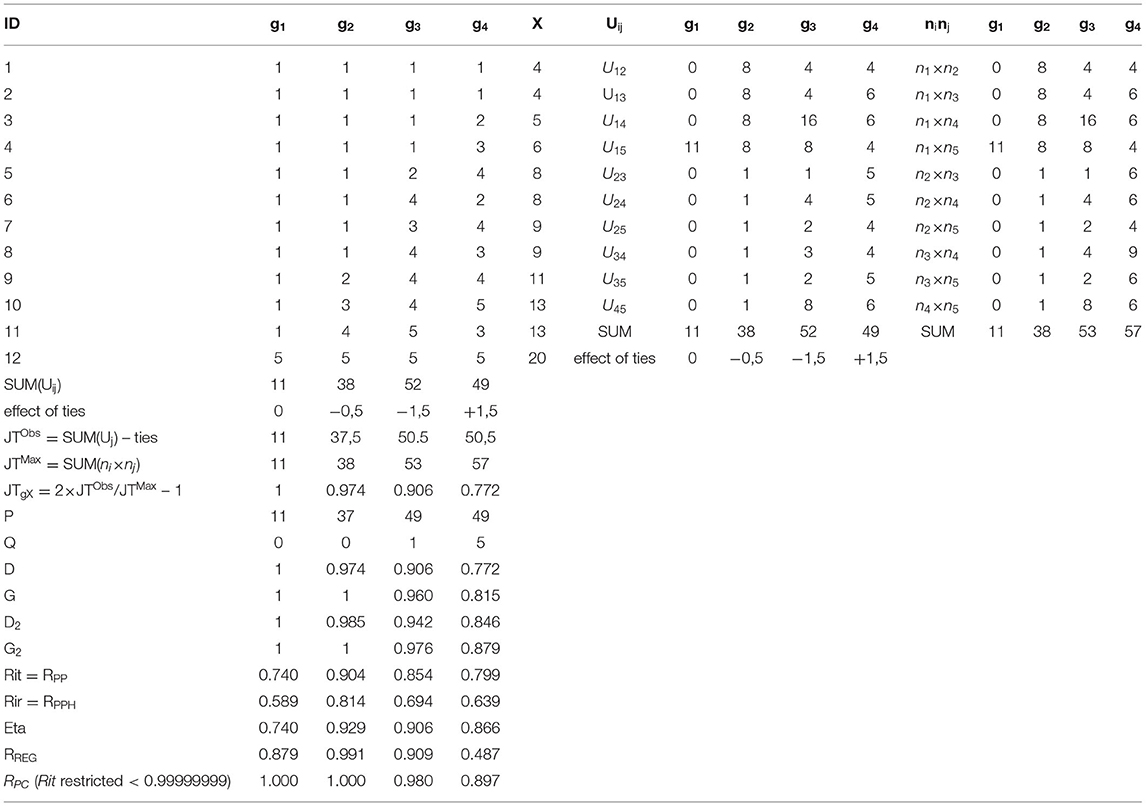
Table 2. A hypothetic dataset to illustrate the computing of coefficients of rank–polyserial correlation.

Item g₁ represents items with an extreme “difficulty” level where we expect to see obvious underestimation by Rit, Rir, and coefficient eta (see [2]). With these kinds of items, G and D, and consequently, JT_gX detect the deterministic pattern as G = D = JT_gX = 1. Item g₂ is a deterministic one, but it includes a minor tie in X, and, hence, the estimate by D = JT_gX is expected to give a slightly more conservative estimate of the association in comparison with that by G. Items g₃ and g₄ have both tied cases and error in the order, and, hence, both G and D are expected to give estimates with the magnitude of $\widehat{D}<\widehat{G}<1$. In all cases, the estimates by G₂ and D₂ are expected to be higher than those by G and D.

The manual calculation of the estimates of the coefficients is discussed by using item g₄ as an example. The statistics related to Wilcoxon's statistics are seen in Table 3 and the contingency table of g₄ × X in Table 4.

TABLE 3

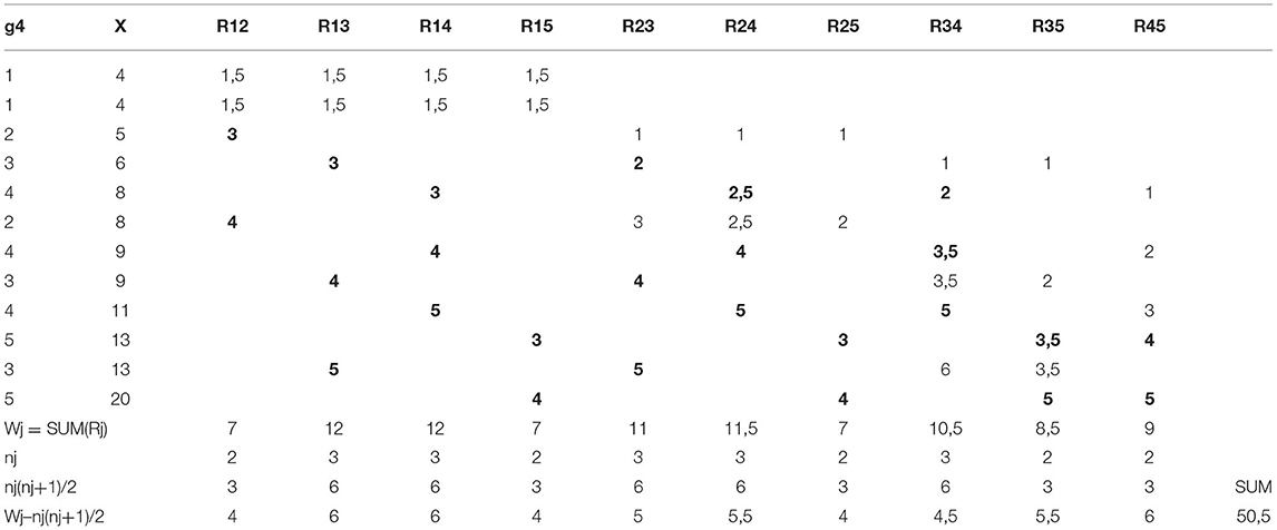
Table 3. Rank-orders (R) in different pairs of i, j between variables g4 and X; the ranks of the higher sub-population j are highlighted.

TABLE 4

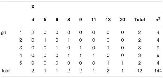
Table 4. Crosstable of variables g₄ and X.

JT_gX

By using the heuristics of U-test statistic, assuming no ties, the sum of the statistics U_g4Xij equals 49 and the ties add 1.5, totaling to $J{T}_{gX}^{Obs}$ = 50.5 (Table 2). The same is obtained strictly by using the routine of Wilcoxon (Eq. 7; see Table 3). The maximal value is $J{T}_{g_{4}X}^{Max}={\displaystyle \sum _{i<j}^r}{n}_i{n}_j=57$ (Eq. 9; Table 2). This can be obtained also by using Eq. (14) and Table 4: the maximum value is $J{T}_{gX}^{Max}=\frac{1}{2}\left[N^2-{\displaystyle \sum _{i=1}^r}\left({n_i}^2\right)\right]=\frac{1}{2}\times \left[144-(4+4+9+9+4)\right]=114/2=57$. Then, JT_g4X = $2\times \left(J{T}_{g_{4}X}^{Obs}/J{T}_{g_{4}X}^{Max}\right)-1$ = 2 × (50.5/57)−1 = 0.772. The core in the estimator, $J{T}_{g_{4}X}^{Obs}/J{T}_{g_{4}X}^{Max}$ = 50.5/57 = 0.886 indicates that 88.6% of the observations in item g₄ are logically (ascending) located after they are ordered by the score X.

For Table 2, the estimates by JT_gX were computed manually by using the information from Table 2. However, in real-life settings, JT_gX has the identity of D(g|X). Then, it is easy to use traditional software packages, such as IBM SPSS, Stata, SAS, or R-packages for calculation. For instance, with IBM SPSS, the syntax for D is CROSSTABS /TABLES = item BY Score/STATISTICS = D. In Stata, a module by Newson [54] is available. In SAS, the command PROC FREQ provides D by specifying the TEST statement by D, SMDC and R options. Correspondingly, in R, D can be computed by Somers Delta (x, y = NULL, direction = c(“row,” “column”), conf.level = NA, ...) (see https://rdrr.io/cran/DescTools/man/). From the output, the option “X dependent” is selected.

D and G

When it comes to coefficients D and G, statistics P and Q are needed for the manual calculation. These can be computed by using a contingency table (Table 4). By using the strategy of “count all entries that lie to the ‘Southeast’ of the particular entry” (see the manual calculation, e.g., [33, 37]), the number of pairs in the same direction is P = (2×) 49. Parallel, the number of pairs in the opposite directions is counted by using the strategy of “count all entries that lie to the ‘Southwest’ of the particular entry”: Q = (2 ×) 5. Consequently, 2 × (P – Q) = 2 × 44 and 2 × (P + Q) = 2 × 54. The number of all pairs in the direction of “g given X” is $D_g={12}^2-\left(2^2+2^2+3^2+3^2+2^2\right)=144-30=114$. Then, G = 44/54 = 0.815 and D(g₄|X) = (2 × 44)/114 = 0.772. Notably, the latter equals the estimate by JT_g4X because of Eq. (22).

For Table 2, the estimates by D and G were calculated manually based on contingency tables. In traditional software packages, such as IBM SPSS, for instance, the syntax for G is CROSSTABS/TABLES = item BY Score/STATISTICS = GAMMA and the syntax for D is CROSSTABS/TABLES = item BY Score/STATISTICS = D. In Stata, the command tabulate g X [if] [in] [weight] [,gamma] produces G (see [55]), and Newson's module [54] produces D. In SAS, the command PROC FREQ provides G and D by specifying the TEST statement by GAMMA, D, SMDCR options. Correspondingly, by using R, G can be computed by GoodmanKruskalGamma (x, y = NULL, conf.level = NA, ...) and D by Somers Delta (x, y = NULL, direction = c (“row,” “column”), conf.level = NA, ...) (see https://rdrr.io/cran/DescTools/man/). From the output related to D, the option “X dependent” is selected.

D₂ and G₂

The dimension-corrected rank–polyserial coefficients D₂ and G₂ are based on the observed values of D and G and knowledge of the number of categories in the item. In the case of g₄, df (g) = 5–1 = 4. For the calculation, A = (3/4)³ = 0.421. Then, by using Eq. (31), an estimate of item–score association is D₂(g₄|X) = D₂ = 0.772 × [1 + (1–0.772) × 0.421] = 0.846 and, by using Eq. (29), G₂(g₄|X)= G₂ = 0.815 × [1+ (1–0.815) × 0.421] = 0.879. For Table 2, these were computed manually by using traditional spreadsheet software.

Rit and Rir

When it comes to the benchmarking estimators, the mechanics of PMC are used in the point–polyserial correlation, that is, in item-total correlation for observed association of the item and the score:

$\begin{array}{ll}{\rho }_{PP}={\rho }_{gX}=Rit=\frac{{\sigma }_{gX}}{{\sigma }_g{\sigma }_X}& (32)\end{array}$

and in Henrysson's item–the rest correlation

$\begin{array}{ll}{\rho }_{PPH}={\rho }_{gP}=Rir=\frac{{\sigma }_{gP}}{{\sigma }_g{\sigma }_P}& (33)\end{array}$

where σ_gX, σ_g, and σ_X are covariation and standard deviations of the item (g) and the score (X), and σ_gP are the covariation and standard deviation of the item g and modified score P where the item in interest has been omitted from the compilation.

For item g₄, the estimates are Rit = 0.799 and Rir = 0.639. In the real-life testing settings, the magnitude of the estimates by Rir is always lower than those by Rit (see algebraic reasons in, e.g., [56]), and both estimators underestimate item–score association when the scales are not equal (e.g., [29]) as is the case with g₄ and X. From this viewpoint, it is known that in the hypothetical example in Table 2, D needs to underestimate the association in an obvious manner as 0.772 < 0.799; this type of obvious underestimation was the reason why the dimension-corrected estimators D₂ and G₂ were developed (see the discussion in [25, 45, 49]). In the case of g₄, the estimate by G (0.815) exceeds the one by Rit. However, this is not true in general; when the number of categories in an item exceeds 4 as here, in real-life testing settings, G tends to give estimates that are lower in magnitude than those by Rit (see [29]; see also later Figure 3).

FIGURE 3

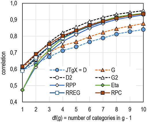
Figure 3. Average estimates by the number of categories in the item (k =14,888 items).

For Table 2, the estimates by Rit and Rit were computed manually by using standard spreadsheet software. Both indices are defaults for the classical item analysis in the widely used general software packages, such as IBM SPSS [50], SAS (e.g., [57]), STATA [55], and in some libraries of R (e.g., [58, 59]).

Eta

Coefficient eta is a close sibling to Rit; with binary and dichotomous items, eta = Rit (see [60, 61]), and with polytomous items Rit follows closely the direction of η(g|X), henceforth, just eta, usually denoted as “X dependent”—which is the same direction as in D(g|X)—and not the opposite direction η(X|g) (see [2]). This is its traditional direction in settings related to GLM (“X dependent”). One of the advances of eta over Rit is that, unlike Rit, eta can detect the possible non-linear pattern in the item, and, hence, in the polytomous settings, the magnitudes of the estimates by eta are always somewhat higher than those by Rit (see the algebraic reasons in, for example [2]).

The traditional form for is

$\begin{array}{l}\eta \left(g|X\right)=\sqrt{{\eta }_{g|X}^2}=\sqrt{\frac{S{S}_{between}\left(g|X\right)}{S{S}_{total}\left(g|X\right)}}\\ =\sqrt{\frac{{\displaystyle \sum _{g=1}^r}{n}_g{\left({\stackrel{-}{X}}_{Xg}-G{M}_X\right)}^2}{{\displaystyle \sum _{i=1}^r}{\displaystyle \sum _{j=1}^c}{\left(x_{ij}-G{M}_X\right)}^2}}& (34)\end{array}$

(e.g., [62]) where ${\stackrel{-}{X}}_{Xg}={\displaystyle \sum _{j=1}^{n_g}}\frac{y_j}{n_g}$ refers to the means of X in different categories in g, and $G{M}_x={\displaystyle \sum _{g=1}^R{n}_g}{\overline{X}}_{Xg}/{\displaystyle \sum _{g=1}^R{n}_g}$ is the grand mean of X. However, Metsämuuronen [2] suggests that a better form—also considering the possible negative values of eta—would be

$\begin{array}{ll}\eta \left(g|X\right)=sign(R_{PP})\times \sqrt{\frac{S{S}_{between}\left(g|X\right)}{S{S}_{total}\left(g|X\right)}}& (35)\end{array}$

This is a relevant modification because using variances in the estimation of eta automatically leads to a positive outcome even if the true association would be negative.

In Table 2, the identity of eta and Rit is seen in g₁(0.740), which is, factually, a dichotomous item because only two categories are obtained. In the case of g₄, the magnitude of the estimate by eta is notably higher [η(g|X) = 0.866] than that by Rit (ρ_gX= 0.799).

For Table 2, the estimates by eta were computed by using IBM SPSS software by using the syntax Crosstabs/Tables = g by X/Statistics = ETA. In Stata, the positive values of eta can be obtained by taking the square root of eta squared obtained by the command estatesize after the ANOVA command. In SAS, the positive values of eta can be found by taking the square root of etasquared after PROC GLM with the option EFFECTSIZE. Correspondingly, by using R, eta is computed by eta (x, y, breaks = NULL, na.rm = FALSE) (see https://rdrr.io/cran/ryouready/man/eta.html).

R_PS

The parametric polyserial coefficients of correlations are the natural counterparts for the robust rank–polyserial coefficients of correlation. While the previous estimators are intended to estimate observed correlation, R_PS is intended to estimate the inferred correlation between a latent g and observed X. In the early years of item analysis, the traditional R_PS was the most used estimator of the item–score association (see [24]). However, from early on, it was known that the traditional way of estimating R_PS leads to obvious overestimation with out-of-range values if the embedded ρ_gX and σ_g are high to start with (R_PS>>1.000). During the years, Clemans [24], Turnbull [63], Brogden [64], and Henrysson [65], as examples, offered solutions to the challenge of overestimation (see the history in [28]). By far, the most promising option in this family is a coefficient called r-polyreg correlation (R_REG; see [27, 28]), which produces estimates that do not exceed 1, nor does it rely on bivariate normality assumptions. It has shown to be very resistant to deflation, although, with short scales in X, it seems to give underestimations (see [29]; see also later Section Comparison of the Estimates With a Larger Dataset).

For the general interest, the traditional estimates by R_PS were computed for the items in Table 2, although they are not seen in the table. The estimates are ρ_{PS_g1} = 1.334, ρ_{PS_g2} = 1.120, ρ_{PS_g3} = 0.945, and ρ_{PS_g4} = 0.841. The two first ones are, obviously, out of range in magnitude, and there is a reasonable doubt also with the other estimates. In Table 2, the estimates by R_REG are seen. By using R_REG in estimating the inferred association related to the item g₁, the estimates are notably higher in magnitude (0.879) than those by Rit, Rir, and eta (≤0.740), although the magnitude is far lower than those by G, G2, and R_PC (1.000), which are known to detect the deterministic pattern accurately (see [29, 45]). With g₂, also with a deterministic pattern, the estimate by R_REG (0.991) is very close to those by G, G2, and R_PC (1.000). With g₃, the estimate by R_REG (0.909) is close to that by D (0.906) but lower than those by G (0.960) and R_PC (0.980). Notably, with item g₄, R_REG seems to underestimate association in an obvious manner (0.487).

The traditional R_PS can be obtained by the two-step procedure introduced by Olsson et al. ([1], see also [23]) where, in the first phase, the marginal proportions of the categorical ordinal variable (p_j) are used to obtain the threshold estimates (γ_j), and these are used, in the second phase, to give estimates by R_PS. The estimate by R_PS can be obtained by

$\begin{array}{ll}{\rho }_{PS}=\frac{{\rho }_{gX}\times {\sigma }_g}{{\displaystyle \sum _{j=1}^r}\Phi \left({\gamma }_j\right)\left(g_{j+1}-g_j\right)}& (36)\end{array}$

(e.g., [23]) where ρ_gX is the point–polyserial correlation between g and X, σ_g is the standard deviation of the categorical ordinal variable, ${\gamma }_j={\Phi }^{-1}(p_j)$ is the inverse of the standard normal density, $\Phi ({\gamma }_j)={(2\pi )}^{-1/2}exp(-{\gamma }^2/2)$ is the standard normal density, and g_j is the category in the ordinal variable g. The last is not needed when all the categories are met as they are in items g₂ – g₄; in these cases, g_j+1-g_j = 1. However, in item g₁, g_j+1 – g_j = 5 – 1 = 4.

For computing R_REG, a statistic β_i is needed. This is the slope parameter of the probit regression model P(x_i ≤ 1|y) = Φ(a_i − β_iy) where Φ is the standard normal cumulative distribution function and a_i and β_i are intercept and slope parameters. The β-value can be computed, for example, in IBM SPSS software using the syntax

$\begin{array}{l}\text{Genlin g}(\text{Order }=\text{ Ascending})\text{ With X/Model X}\\ \text{Distribution }=\text{ Multinomial}\\ \text{Link }=\text{ Cumprobit/}\\ \text{Criteria Method }=\text{ Fisher/Print Solution.}\end{array}$

After the estimates of β and the population variance of the score variable X ($\widehat{\beta }$ and ${\widehat{\sigma }}_X^2$, respectively) are computed, R_REG is estimated as

$\begin{array}{ll}{\rho }_{REG}=\frac{\widehat{\beta }{\widehat{\sigma }}_X}{\sqrt{{\widehat{\beta }}^2{\widehat{\sigma }}_X^2+1}}& (37)\end{array}$

For Table 2, the β values were computed by using SPSS software, and the estimates of ${\sigma }_X^2$ and R_REG were computed manually by using a spreadsheet software package. Note that the standard outputs of generally known software packages produce, usually, the sample variance$s_X^2$. This is transformed into the “population” variance by multiplying the outcome with (N − 1)/N. If using MS-Excel, as an example, we can select whether the sample variance (= VAR.S) or population variance (= VAR.P) is used. The latter is used in Table 2.

R_PC

As R_BS above, also the parametric coefficient of correlation is a natural counterpart for the nonparametric or robust rank–polyserial (or polychoric) coefficients of correlation. R_PC differs from the previous ones in that no closed-form expression for the relation between R_PP and R_PC is available. Instead, several alternatives for the process to obtain the estimates are suggested, which produce slightly different estimates (see [23]). As an estimator of correlation, R_PC is advantageous over R_PP, specifically, with ordinal datasets (e.g., [66–69]), and it is very resistant against several sources of deflation (see [29, 45]). Also, it is robust in accurate reproduction of the measurement models with unbiased standard errors even in small sample sizes (e.g., [66–68]).

One practical challenge in from the item analysis viewpoint is that we do not know what kind of composite the item discrimination refers to; the estimates refer to hypothetical composites to the research is not privy to (see [25, 70]). Also, the computational challenges are well-known; the estimation needs complicated procedures (e.g., [71]). Additionally, the established routines for estimating ρ_PC (e.g., [19–22]) cannot reach the extreme values +1 and −1 because the deterministic patterns lead to computational problems. The last challenge is easy to solve though (see below the restrictions used in estimation).

In reference to Table 2, R_PC accurately detects the deterministic patterns in items g₁ and g₂. This is expected by its behaviour in simulations (e.g., [29, 45]). Also, the magnitudes of the estimates in g₃ and g₄ (0.980 and 0.897, respectively) seem to be quite close to those by G₂ (0.976 and 0.879, respectively). Hence, if the estimates by R_PC are taken as the closest approximation of the latent variables manifested in ordinal or interval-scaled form, it seems that, of the options for rank–polyserial coefficients of correlation, G₂ could be taken a quite close match to R_PC. In-depth studies are needed to confirm this. Some light on this matter is given in the next section, with a comparison with a larger dataset.

In IBM SPSS [50], the syntax for R_PC is not available, although some macros have been published (e.g., [72]). In SAS, the command PROC CORR provides R_PC. Correspondingly, in R, R_PC can be computed by CorPolychor (x, y, ML = FALSE, control = list(), std.err = FALSE, maxcor = 0.9999)## S3 method for class “CorPolychor” print (x, digits = max (3, getOption (“digits”)-3),...) (see https://rdrr.io/cran/DescTools/man/CorPolychor.html). In computing the estimates in Table 2, the two-step estimator by Martinson and Hamdan [20] was used. Simplified by Zaionts [73], the task is to find an estimate of R_PP = ρ_gX, which maximises the log-likelihood function LL, where

$\begin{array}{ll}LL={\displaystyle \sum _{g=1}^r}{\displaystyle \sum _{X=1}^c}{n}_{gX}LN\left[P\left(g=i,X=j\right)\right]& (38)\end{array}$

In the first step, the threshold coefficients γ_i and τ_j are estimated for both g and X, and in the second step by iteration, we find R_PP that maximises LL. The estimates were computed manually by modifying Zaionts' [73] procedure for MS-Excel: Rit was restricted to be Rit < 0.99999999, and, in each operation with logarithm, an additional 0.000000001 was added. The latter is for the cases of deterministic patterns, causing value 0 in the cell; the logarithm of zero is not defined. Hence, technically, R_PC cannot reach the ultimate correlation. In Table 2, this is denoted by value 1.000 instead of 1 as with G and G₂.

Comparison of the Estimates With a Larger Dataset

The coefficients of R_RP are compared with relevant estimators by using 6,932 real-world items from 1,440 datasets. The estimators are studied from three viewpoints. First, how the factual estimates differ from each other in different situations by varying the number of categories in the item and the score, varying the item difficulty, and varying the number of observations in the sample. Second, the estimators are compared from the viewpoint of how efficiently they reflect the population value. Third, the estimators are briefly compared related to their tendency to resist deflation as estimators of the item–score association.

Empirical Real-Life Datasets Used in the Comparison

The dataset used in the comparison is a public one. The dataset of 14,888 estimates of item–score association is published at doi: 10.13140/RG.2.2.10530.76482 in CSV format and at doi: 10.13140/RG.2.2.17594.72641 in SPSS format. Of these items, 6,932 are polytomous, and these are used in the comparison.

The datasets are formed by different compilations of 20–30 binary items and their sums forming items with 2 to 15 categories (to form polytomous items). Randomly selected test-takers of n = 25, 50, 100, and 200 were picked from a nationally representative dataset of a mathematics test for Grade 9 [74] with N = 4,023. The items and scores formed 1,440 tests with different numbers of test-takers (n), test lengths (k), difficulty levels ($\stackrel{-}{\text{p}}$), reliabilities (α), and a number of categories in the items and scores [df (g) and df (X), respectively].

Comparison of the Estimates in Varying the Conditions

First, an obvious lift of the comparison of the estimators is that the estimates by JT_gX = D and G underestimate item–score association in an obvious manner when the number of categories exceeds 3 (in D) and 4 (in G) (see Figure 3 also including the binary items; see Table 1 in Supplementary Appendix 2). This is also known by previous simulations (e.g., [29, 45]). The phenomenon is known from the fact that the estimates by R_PP are always deflated whenever the scales are not identical in two variables (see the algebraic reasons in [75, 76]) as is always the case with an item and a score. Notably, the magnitude of the estimates by R_PP tends to exceed those by D and G with items with a wide scale.

Second, the estimates by D₂ tend to be close to those by R_REG and R_PC, and the estimates by G₂ tend to be slightly higher than those by R_PC regardless of the number of categories in the items. These are not general characteristics though. It is to be seen that, more frequently, the magnitude of the estimates by D₂ tends to be close to those by R_REG and the magnitude of the estimates by G₂ tends to be close to those by R_PC.

Third, the binary case is given as a benchmark here; the estimates by R_PP and eta are notably deflated with the binary dataset. With the special case suitable for a point–biserial correlation, all other estimators than R_PP and eta would produce closely the same estimate. The differences between the estimators come with items with a wide scale [df (g) > 3]. In what follows, the binary cases are omitted, and just k = 6,932 items with polytomous nature are used in the study.

Regarding the number of categories in the score, it seems that the estimates are stable if the score has more than 15 categories (Figure 4; see Table 2 in Supplementary Appendix 2). If the number of categories is less than 16, all the estimators tend to produce unstable estimates. The instability in the estimates with tests with a narrow scale in a score is discussed later with the efficiency of the estimators to reflect the population value. When it comes to the magnitude of the estimate, the estimators seem to form three groups. With scores wider than 15 categories, R_RP based on D tends to give estimates with notably lower magnitude than the other estimators. R_RP based on G tends to give estimates that are at the same level as those by R_PP and eta. R_RP based on G₂ and D₂ tends to give estimates that are at the same level as those by R_REG and R_PC. Of these estimators, the magnitude of the estimates by D₂ tends to follow closely those by R_REG, and the magnitude of the estimates by G₂ tends to follow those by R_PC.

FIGURE 4

Figure 4. Average estimates by the number of categories in the score (k = 6,932 items).

When it comes to the difficulty levels of the items, the traditional R_PP and eta include obvious deflation in estimates with extremely easy and difficult items—and in the binary case, as discussed in Figure 3 (Figure 5, see Table 3 in Supplementary Appendix 2). The phenomenon is known from the previous simulations (e.g., [25, 29, 45, 49]). In the given dataset, this phenomenon is indicated by the notably lower magnitude of the very easy items—extremely difficult polytomous items were not obtained in the polytomous dataset. The magnitude of estimates by JT_gX = D and G tends to be lower than by the other estimators with items of medium difficulty levels, but, with items with extreme difficulty levels, they tend to not differ from those by the other estimators. This is caused by the fact that the probability to obtain deterministic patterns is high with items with extreme difficulty levels. Then, the magnitude of the estimates by D and G tends to get closer to D₂ and G₂. Correspondingly, the magnitude of the estimates by D₂ and G₂ does not differ notably from the benchmarking estimators R_REG and R_PC.

FIGURE 5

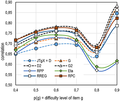
Figure 5. Average estimates by the item difficulty (k = 6,932 items).

When it comes to sample size, all estimators tend to give stable estimates when the sample size n = 50 is reached (Figure 6; see also Table 3 in Supplementary Appendix 2). When the sample size is very small (n = 25 in the dataset), the magnitudes of the estimates are deflated. As above, the magnitude of the estimates by D₂ tends to follow closely those by R_REG, and the magnitude of the estimates by G₂ tends to follow those by R_PC. The estimates by D, G, RPP, and eta tend to be deflated in comparison with R_PC and G₂. The estimators of R_RP form four distinguished estimators when it comes to magnitude of the estimates. Coefficient D is known to be the most conservative of the options for R_RP, and, hence, the magnitude of the estimates by JT_gX and D is the lowest in comparison. Coefficient G is more liberal than D, and the magnitudes of the estimates tend to follow the tendency of R_PP and eta when the number of sample size exceeds n = 50. Coefficient D₂ is somewhat more conservative in comparison with G₂, but the magnitudes of the estimates are notably higher than those by D and G. Notably, with very small sample size (n = 25 in the dataset), the magnitude of the estimates by D₂ seems to be very close to those by eta, and, when the sample sizes reach n = 50, the magnitude starts to follow the tendency of R_REG. The highest magnitudes of the estimates are given by G₂, and its trend follows closely the tendency by R_PC.

FIGURE 6

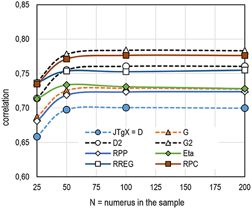
Figure 6. Average estimates by the number of cases in the sample (k = 6,932).

To condense the results by far, it seems that, with items with wide or wide-ishscale (more than 3–4 categories), the estimators JT_gX = D and G tend to underestimate item–score association in an obvious manner, while the magnitude of the estimates by D₂ tends to be close to those by R_REG, and magnitude of the estimates by G₂ tends to be close to those by R_PC. The magnitudes of the estimates tend to be as follows:

$\begin{array}{ll}J{T}_{gX}=\widehat{D}<\widehat{G}<{\widehat{D}}_2<{\widehat{G}}_2& (39)\end{array}$

This order is expected because of the known characteristics of the estimators; the estimates by D are more conservative than those by G (see, e.g., [45]), and the estimates by D₂ are more conservative than those by G₂ (e.g., [29]).

Efficiency of the Estimators to Reflect the Population Value

The efficiency of the estimators of R_RP and related benchmarking estimators to reflect the population value is studied by comparing the sample and “population” estimates computed from the original real-world dataset of 4,023 test-takers. As a combination of different sets of items, the procedure for producing the simulation dataset came up with 137 different score variables related to polytomous items. These all produce slightly different population values. The average estimates are collected in Table 5.

TABLE 5

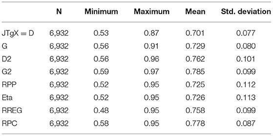
Table 5. Average “population” estimates for the comparison.

Because we do not know the real population value of item–score association in the real-life datasets, each estimator races its own race against itself: D from the sample is compared with the corresponding D from the population, as an example. A simple and straightforward statistic is computed: the difference (d) between the sample estimate and the population estimate. If d > 0, the population value was overestimated, if d = 0, the estimate was equal in the sample and the population, and if d < 0, the population value was underestimated. This statistic is denoted as d in the name of the coefficient: dD refers to a difference between the sample D and population D.

When it comes to the number of categories in the item, the first point to make is that the estimates by D₂ and G₂ are the least effective in reaching the population value—they tend to underestimate the population value the greatest (Figure 7; see Table 5 in Supplementary Appendix 2). In contrast, second, the estimates by eta tend to be overestimated with items with wide scales. This is an interesting phenomenon, knowing that eta tends to give obvious underestimates in the same manner as R_PP does. It means that the wider the number of categories gets, the more probable it is to find association by eta from the population (or in large sample size), with a lower magnitude in comparison with the sample estimates. This seems to be the opposite with D₂ and G₂. Third, except R_REG, all estimators in comparison share the common characteristic that the narrower the scale in item (up to 8 categories) is, the more the estimator tends to underestimate the population parameter up to 0.02 units of correlation. R_REG seems to be surprisingly robust against the effect of the scale in item; regardless of the length of the scale, the estimates tend to be very close to the population value.

FIGURE 7

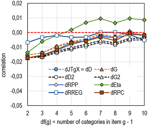
Figure 7. Average difference between the sample and population by df(g) (k = 6,932 items).

When it comes to the number of categories in the score, above, it was noted that, when the number of categories in the score exceeds 15, the estimates tend to be stable. From the perspective of reflecting the population estimate, except R_REG, all estimators tend to notably underestimate item–score association with tests with a narrow scale in the score, that is, when df (X) < 15 (Figure 8, see Table 6 in Supplementary Appendix 2). In this respect, there seem to be no differences between the estimators except that R_REG produces robust estimates and eta does not underestimate the association as much as the other estimators.

FIGURE 8

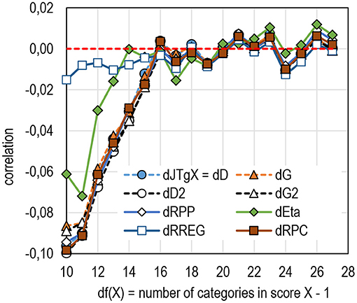
Figure 8. The average difference between the sample and population by df(X) (k = 6,932).

When it comes to the difficulty of the items, all estimators tend to underestimate the population correlation with difficult items (Figure 9, see Table 7 in Supplementary Appendix 2), and the underestimation may be notable up to 0.09 units of correlation. Notably, the dataset used in the comparison does not include polytomous items, with an extreme difficulty level; it is possible that, with more extreme (difficult) items, the underestimation may be more drastic. Notably, with extremely easy items, the underestimation is not as radical as with extremely difficult items (<0.02 units of correlation). Systematic studies in this respect would be beneficial. In this respect, there are no notable differences between the estimators of R_RP —all are conservative. Again, it seems that R_REG is more robust than the other estimators.

FIGURE 9

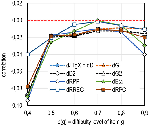
Figure 9. The average difference between the sample and population by the item difficulty (k = 6,932).

Finally, when it comes to the sample size, except eta, all estimators tend to be conservative; they underestimate the population estimate (Figure 10; see also Table 8 in Supplementary Appendix 2). With a very small sample size (n = 25), the underestimation is notable (0.04–0.05 units of correlation), and, when the sample size is n = 50 or higher, all estimators tend to give estimates that are close to the population estimate. The pattern is notably identical with all estimators except R_REG and eta; the sample eta overestimates mildly the population eta (<0.005 units of correlation) and the population R_REG gives roughly the same estimate as is the population R_REG regardless of the sample size.

FIGURE 10

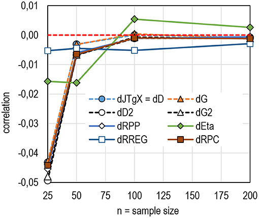
Figure 10. The average difference between the sample and population by the sample size (k = 6,932).

Deflation in the Estimates

General Measurement Model Related to Deflation in Estimators of Correlation

It is a well-known fact that PMC is prone both to attenuation caused by errors in measurement modelling and to radical deflation caused by a technical or mechanical errors in the calculation process. These concepts are discussed, amongst others, by Chan [77], Gadermann et al. [78], Lavrakas [79], and Metsämuuronen [26, 30, 80].

Both attenuation and deflation in PMC are artificial and systematic. Sometimes, attenuation has been connected to the phenomenon called restriction of a range or range restriction (see literature, e.g., in [81–84]). Pearson (5) himself was the first to offer a solution to the attenuation problem, and many solutions have been offered to correct the attenuation in the X variable (see the typology in [82]). However, even if there is no manifestation of range restriction in X in the sense discussed by Sacket et al. [82], PMC is very vulnerable to several sources of mechanical error in the estimates of correlation causing deflation. Metsämuuronen [29, 45] found seven such sources: (1) the division of subpopulations in g (or item difficulty in the measurement modelling settings), (2) the discrepancy in scales of the variables, (3) the distribution of the latent variable, (4) the number of categories in g, (5) the number of categories in X, (6) the number of items forming the score, and (7) the number of tied cases in the score. In practical terms, the deflation is obvious when assuming two identical normally distributed variables with obvious perfect correlation. If we dichotomized one variable (g) and polytomize the other (X), PMC and many other estimators based on covariation cannot reach the (obvious) perfect (latent) correlation (see the algebraic reasons for PMC in [75, 76], and for coefficient eta in [2]). The deflation, that is, the underestimation of the true latent association because of technical or mechanical reasons is the greater the more extreme is the division (or the difficulty level) in g.

While the effect of attenuation may be nominal in the dataset, deflation in PMC = R_PP may be radical; it approximates 100% if the variance in the item is small, that is, with an item with an extreme difficulty level, causing a small item–total covariation; this is strictly inherited by the formula of PMC (see Eq. 32). To make this radical deflation visible in the measurement model, Metsämuuronen [26, 29, 30] has proposed a general measurement model, combining a latent variable (θ), observed values of an item (x_i), and a weight factor w_iθ that links θ with item i, and the measurement error e_iθ:

$\begin{array}{ll}{x}_i=w_{i\theta }\theta +e_{i\theta }& (40)\end{array}$

generalised from the traditional measurement model (see, e.g., [85, 86]).

In the general model, the unobservable θ may be manifested as a varying type of relevantly formed compilation of items, including a theta score formed by the raw score (θ_X), a principal component score (θ_PC), a factor score (θ_FA), item response theory (IRT) or Rasch modelling (θ_IRT), or various non-linear combination of the items (θ_Non−Linear). The weight factor w_iθ is a coefficient of correlation in some form, also including a principal component and factor loadings (λ_i). In a normal case, w_iθ varies −1 ≤ w_iθ ≤ +1; values higher than +1 or smaller than −1, sometimes obtained by bi- and polyserial correlation or by factor loadings, are taken out-of-range values.

The mechanical error in the estimation of correlation leading to deflation in the estimates has been re-conceptualised in the measurement model as

$\begin{array}{ll}{x}_i=w_i\times \theta +\left(e_{i\text{\_}Random}+e_{wi\theta \text{ \_}MEC}\right)& (41)\end{array}$

(e.g., [29]), where the notation in the element e_{wi θ _MEC} refers to the fact that the magnitude of deflation caused by the mechanical error in the estimation (MEC) depends on the weighting factor w, item i, and score variable θ. This characteristic of the rank–polyserial coefficients of correlation is discussed in what follows.

Deflation in the Estimates of R_RP

Based on a simulation of 11 sources of mechanical error, causing deflation in estimates of the item–score association [29], of the options for R_RP, the estimators D and D₂ were noticed to be the most prone to deflation, while the estimators G and G₂ tended to be close to be deflation free. Of the benchmarking estimators, R_PC appeared to be close to deflation free, while R_REG is mildly defected by the number of categories in the item and the score, the distribution of the latent variable, and R_PP is severely affected by several sources of deflation. That D and D₂ were ranked lower in comparison is caused by the fact that, in a theoretical dataset with identical latent variables, D and D₂ tend to be sensitive to the number of categories in the item and the score as well as for the distribution of the latent variable (see Table 6). However, in real-life datasets, as seen in the previous sections, the factual magnitude of the estimates by D₂ tends to follow the magnitude of those by R_REG (see Section Comparison of the Estimates With a Larger Dataset).

TABLE 6

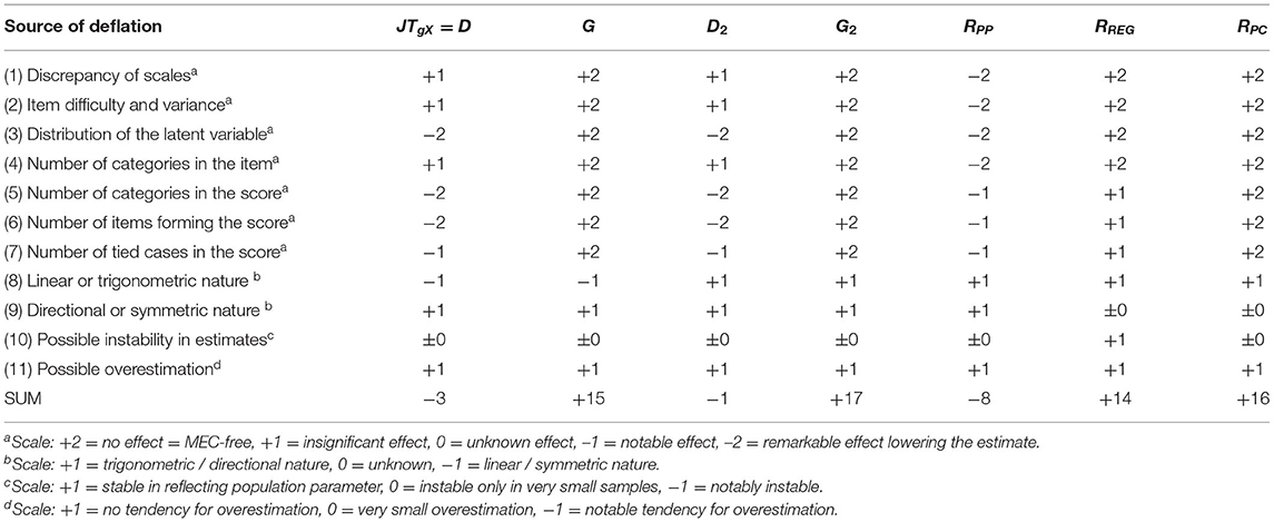
Table 6. Sensitivity of the estimators of R_RP to deflation (based on Metsämuuronen [29]).

Simulations have shown that such coefficients of correlation in Table 1 related to PMC as R_PP and coefficient eta include a notable magnitude of deflation in the estimates (see [2, 29, 45]). This can be easily verified by using a simple example related to Figure 2 and the related discussion. Take two identical variables with a continuous scale, and they (obviously) have a perfect correlation (ρ_θθ = 1). In the case we truncate one into 5 categories as in Section Simple Comparison of the Options for R_RP (categories 1–5; Item g) and the other into more than two categories (Score X); these estimators of association cannot reach the factual latent correlation. Depending on the cut-offs of the values in g, that is, the “difficulty level” of the items and the number of categories in X, the deflation in the estimates may be notable, approximating 100% with extremely difficult items. In contrast, such estimators as R_PC, R_REG, G, and D include notably less mechanical error (MEC) than Rit if not being MEC free (see [29, 45]). This phenomenon of deflation is illustrated in Figure 11.

FIGURE 11

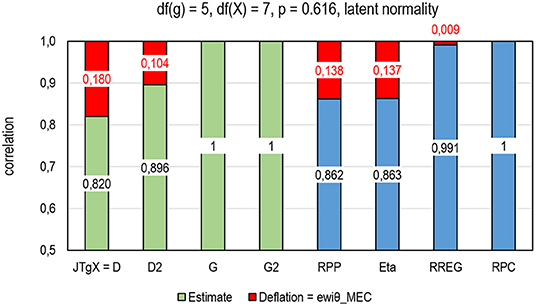
Figure 11. Deflation in the estimates in an item with p = 0.616, df(g) = 4, and df(X) = 7, latent normality, n = 1,000.

Let us assume an item close to g₄ in Table 2. Two identical variables with 1,000 cases with a normal distribution are truncated so that the other includes 5 categories [df (g) = 4] and the other 8 categories [df (X) = 7], and the cut-offs in the item are selected so that p = 0.616⁷. Figure 10 presents the estimates. The outcome is that, if we would have two perfectly correlated variables and their technical manifestations would have been like in g₄, we would expect that an estimate by D would have deflation of 0.180 units of correlation and D₂ would have deflation of a magnitude of 0.104 units of correlation. Correspondingly, G and G₂ can detect the perfect latent correlation in the same manner as RPC does—no deflation is detected. Of the benchmarking estimators, RREG includes a minor amount of deflation (0.009), while RPP and eta include a notable magnitude of deflation (0.138 and 0.137 units of correlation, respectively. This phenomenon explains—at least partly—why the magnitude of the estimates by D is lower than those by G, for example.

All in all, referring to the measurement model in Eq. (40) and the element e_{wiθ_MEC} related to the deflation caused by the mechanical error in the estimating process (MEC), we end up with the following relation of the deflation in the estimators of R_RP: e_{JTgXi_MEC} = e_{Di_MEC} > e_{D2i_MEC} > e_{Gi_MEC} = e_{G2i_MEC} ≈ 0.

Conclusions and Limitations

Main Results in a Nutshell

This article started with the note that we seem to miss a coefficient of correlation that could be used as the rank–polyserial coefficient of the observed correlation between a categorical ordinal variable and an interval- or ordinal-scaled variable. The quest for finding the “missing” coefficient led us, first, to a new coefficient of correlation, rank–biserial correlation between an ordinal variable g and a metric variable X(JT_gX) that was derived by generalising rank–biserial correlation into polytomous ordinal cases by using Jonckheere–Terpstra test statistics—hence, the name JT_gX. It was shown that two traditional coefficients of correlation, Somers D and Goodman–Kruskal G, are strictly related to JT_gX, and, hence, these also could be considered as rank–polyserial coefficients. Furthermore, two related estimators of correlation, dimension-corrected D and G (D₂ and G₂), are strictly related to D and G, and, hence, those could be considered dimension-corrected coefficients rank–polyserial correlation.

To conclude the outcomes from the empirical section, by using different estimators carrying characteristics of rank–polyserial coefficient, the estimates by JT_gX = D, G, D₂, and G₂ tend to follow the following pattern: The magnitude of the estimates by JT_gX and D is the lowest; D is the most affected by several sources of deflation. The magnitude of the estimates by G tends to be higher than those by D, and the estimates tend to follow the tendency of R_PP and eta when the sample size exceeds n = 50. The magnitude of the estimates by D₂ is higher than those by D and G, and the estimates seem to follow the tendency of R_REG when the sample size exceeds n = 50. The highest magnitudes of the estimates are given by G₂, and its trend follows closely the tendency of the estimates by R_PC.

Hence, on the one hand, if the estimates by R_REG and R_PC are taken as accurate reflections of the latent item–score correlations, rank–polyserial coefficients based on D₂ and G₂ seem to be relevant options to use as R_RP and to study more. These are based on observed variables because the underlying estimators D and G are based on observed variables. On the other hand, rank–polyserial coefficients based on D and G given the possibility of an interesting practical interpretation because of Eqs. (20) and (28): 0.5 × D + 0.5 and 0.5 × G + 0.5 strictly indicate the proportion of logically (ascending) ordered observations in Item g after they are ordered by the score. Hence, if D = 0.90, 95% of the observations (0.5 × 0.90 + 0.5 = 0.95) are logically ordered in the item.

Characteristic of all these estimators proposed as estimators of R_RPis that they all are directional—the same also holds with the rank–biserial correlation. They all indicate to what extent the variable with a wider scale (X)—ordinal, interval, pseudo-continuous, or continuous scale—explains the ordinal pattern in the variable with a narrower ordinal scale (g). In the measurement modelling settings, this can be taken as an advance. After all, the whole apparatus in testing settings is based on the idea that the latent variable manifested as the score variable explains the behaviour in a test item, and the other direction does not make sense. All the options of R_RP discussed in this article are directed to favour this direction. A possible advantage of the new coefficient JT_gX is that it leads us strictly to the correct form of the three alternatives produced by the standard procedures of calculating Somers' D.

Known Limitations

An obvious limitation in the study is that the characteristics of the behaviour of the coefficients were illustrated only by using a limited real-world dataset with very limited sample sizes. Although the sample sizes may be taken relevant from the practical testing setting viewpoint—after all, arguably, most tests in the world are administered in the classroom situation or lectures with a very limited number of test takers. However, controlled simulations with the known true association and with large sample sizes would be beneficial. In this, using the character in D and G to strictly indicate the proportion of logically ordered observations after ordered by the score could be utilised.

The simulation is Section Comparison of the Estimates With a Larger Dataset did not include very difficult items—this is clearly a deficiency in the original dataset. Hence, systematic studies of the behaviour of the options for R_RP with items with extreme difficulty levels would be beneficial.

Data Availability Statement

Publicly available datasets were analysed in this study. This data can be found here: http://dx.doi.org/10.13140/RG.2.2.10530.76482; http://dx.doi.org/10.13140/RG.2.2.17594.72641; http://dx.doi.org/10.13140/RG.2.2.17241.65127; and http://dx.doi.org/10.13140/RG.2.2.20111.30882.

Ethics Statement

Ethical approval was not provided for this study on human participants because the dataset is collected as part of national assessment and evaluation by the National Authority. Dataset is anonymized and used by permission. Written informed consent from the participants' legal guardian/next of kin was not required to participate in this study in accordance with the national legislation and the institutional requirements.

Author Contributions

The author confirms being the sole contributor of this work and has approved it for publication.

Funding

Open access support was provided by Centre for Learning Analytics, University of Turku.

Conflict of Interest

The author declares that the research was conducted in the absence of any commercial or financial relationships that could be construed as a potential conflict of interest.

Publisher's Note

All claims expressed in this article are solely those of the authors and do not necessarily represent those of their affiliated organizations, or those of the publisher, the editors and the reviewers. Any product that may be evaluated in this article, or claim that may be made by its manufacturer, is not guaranteed or endorsed by the publisher.

Supplementary Material

The Supplementary Material for this article can be found online at: https://www.frontiersin.org/articles/10.3389/fams.2022.914932/full#supplementary-material

Footnotes

1. ^The contemporary measurement modelling settings result in score variables that are, factually, categorical ones, either ordinal, interval-scaled, or pseudo-continuous type, with the limited number of categories (see the discussion in, e.g., [2]). To obtain a truly continuous scale necessitates a truly continuous scale in at least one test item and a very large number of test takers. This kind of scale always leads to an even distribution because all test takers will get a unique score. Truly continuous scales are very rare in the testing settings. A raw score forms usually a categorical (ordinal or interval-scaled) score and the one-parameter item response theory (IRT) modelling or Rasch modelling forms a pseudo-continuous score where the number of categories in the score variable equals the number of the raw score, but the “names” of the categories come from a continuous scale. The scores by factor analysis and two- or three-parameter IRT models produce scales with more categories, although these, too, are pseudo-continuous scales where the number of categories is strictly bound to the number of test takers, the number of items, and the number of categories in the items.

2. ^A specific peculiarity in naming of the directions may be necessary to discuss here (see also [2, 29, 32]) because the directional estimators are used in what follows. With the truly directional estimators D and eta, in widely used software packages as IBM SPSS, SAS, and R-libraries, this specific direction is traditionally named as “X dependent” (see, e.g., [15, 33–37]). This naming is relevant in the general linear modelling (GLM) settings related to eta squared where the score cannot explain, for example, the sex of the test takers (g), and, hence, the score X must be a dependent variable. However, opposite thinking for the same direction is used in the measurement modelling settings, where the score variable explains the behaviour in the test item and the other direction does not make sense (see, e.g., [38, 39]). This is the case also in the nonparametric testing with U-test or Jonckheere–Terpstra test, as examples, where the idea is to first order the cases by X, after which the order of the cases in the item is analyzed. Hence, the score explains the order of the observations in g, and then, this direction should be named as “g dependent” or “g given X”. In this article, the notations D(g|X) and η(g|X) refer to the direction of “g given X,” which, in the widely used statistical packages, would be named as “X dependent”.

3. ^In the simplified notation of P and Q, they are usually seen without doubling. Technically though, P and Q are always calculated two times (see, e.g., [32, 51]). Hence, in the form of D, the doubling is seen strictly in the form (Eq. 13), but, in the form on G, both P and Q need to be thought doubled. Hence, 2 × in Eqs. (23) and (24).

4. ^This character is typical for the measurement modelling setting, but it is not relevant in general. Both G and D estimate probability, and this they make without underestimation. However, probability with a linear nature tends to give lower values of association than covariance with a trigonometric nature when two variables are continuous (see discussion in, e.g., [29, 34, 53]). This phenomenon is reflected in the item–score association with polytomous items.

5. ^These are specific coefficients for the measurement modelling settings because they are developed in the settings related to measurement modelling settings, and they are not studied in other contexts. They may be applicable in general settings, too, but more studies are needed to confirm or reject this.

6. ^The directionality of the point–biserial and point–polyserial correlation is generally not known. However, this is obvious because of the relation between PMC and coefficient eta. In the binary settings, R_PB equals η(g|X) and not η(X|g). In polytomous settings, R_PP follows closely the direction of η(g|X) and not that of η(X|g) (see [2]).

7. ^A dataset in CSV format at doi: 10.13140/RG.2.2.17241.65127 and in SPSS format at doi: 10.13140/RG.2.2.20111.30882 is available for the comparison of two identical variables truncated into two different forms. The dataset consists of 22,824 estimates related to three types of a latent variable (normal, even, gamma), different difficulty levels (p = 0.002–0.998), several score variables [df (X) = 5, 7, 13, 21, 26, 31, 41, and 61] and items with df (g) = 1–4, that is, the usual scales from binary to Likert type of scale are covered.

References

1. Olsson U, Drasgow F, Dorans NJ. The polyserial correlation coefficient. Psychometrika. (1982) 47:337–47. doi: 10.1007/BF02294164

CrossRef Full Text | Google Scholar

2. Metsämuuronen J. Artificial systematic attenuation in eta squared and some related consequences. Attenuation-corrected eta and eta squared, negative values of eta, and their relation to Pearson correlation. Behaviormetrika. (2022) 2022:1–35. doi: 10.1007/s41237-022-00162-2

CrossRef Full Text | Google Scholar

3. Cureton EE. Rank–biserial correlation. Psychometrika. (1956) 21:287–90. doi: 10.1007/BF02289138

CrossRef Full Text | Google Scholar

4. Pearson K. Mathematical contributions to the theory of evolution III. Regression, heredity, and panmixia. Philos Trans R Soc Lond Ser A. (1896) 187:253–318. doi: 10.1098/rsta.1896.0007

CrossRef Full Text | Google Scholar

5. Bravais A. AnalyseMathematique. Sur les probabilités des erreurs de situation d'un point. (Mathematical analysis. Of the probabilities of the point errors). Mémoiresprésentés par divers savants à l'Académie Royale des Siences de l'Institut de France (Memoirs presented by various scholars to the Royal Academy of Sciences of the Institute of France) 9:255–332. Available online at: https://books.google.fi/books?id=7g_hAQAACAAJandredir_esc=y (accessed November 6, 2022).

Google Scholar

6. Pearson K. On the Theory of Contingency and Its Relation to Association and Normal Correlation. Drapers' Company Research Memoirs. Biometric Series I, XIII. London: Dulau and Co (1904).

7. Pearson K. I Mathematical contributions to the theory of evolution. XI. On the influence of natural selection on the variability and correlation of organs. Philos Trans R Soc A. Math Phys Eng Sci. (1903) 200:1–66. doi: 10.1098/rsta.1903.0001

CrossRef Full Text | Google Scholar

8. Pearson K. On the General Theory of Skew Correlation Non-Linear Regression. London: Dulau Co (1905). Available online at: https://onlinebooks.library.upenn.edu/webbin/book/lookupid?key=ha100479269 (accessed November 6, 2022).

9. Goodman LA, Kruskal WH. Measures of association for cross classifications. J Am Stat Assoc. (1954) 49:732–64. doi: 10.1080/01621459.1954.10501231

CrossRef Full Text | Google Scholar

10. Goodman LA, Kruskal WH. Measures of association for cross classifications: II. Further discussion and references. J Am Stat Assoc. (1959) 54:123–63. doi: 10.1080/01621459.1959.10501503

PubMed Abstract | CrossRef Full Text | Google Scholar

11. Kendall MG. A new measure of rank correlation. Biometrika. (1938) 30:81–93. doi: 10.2307/2332226

CrossRef Full Text | Google Scholar

12. Somers RH. A new asymmetric measure of association for ordinal variables. Am Sociol Rev. (1962) 27:799–811. doi: 10.2307/2090408

CrossRef Full Text | Google Scholar

13. Glass GV. Note on rank biserial correlation. Educ Psychol Measur. (1966) 26:623–31. doi: 10.1177/001316446602600307

CrossRef Full Text | Google Scholar

14. Wendt HW. Dealing with a common problem in social science: a simplified rank biserial coefficient of correlation based on the U statistic. Eur J Soc Psychol. (1972) 2:463–5. doi: 10.1002/ejsp.2420020412

CrossRef Full Text | Google Scholar

15. Newson R. Identity of Somers' D the Rank Biserial Correlation Coefficient. (2008). Available online at: http://www.rogernewsonresources.org.uk/miscdocs/ranksum1.pdf

Google Scholar

16. Pearson K. Mathematical contributions to the theory of evolution. VII. On the correlation of characters not quantitatively measurable. Philos Trans R Soc A. Math Phys Eng Sci. (1900) 195:1–47. doi: 10.1098/rsta.1900.0022

CrossRef Full Text | Google Scholar

17. Pearson K. On the measurement of the influence of “broad categories” on correlation. Biometrika. (1913) 9:116–39. doi: 10.1093/biomet/9.1-2.116

CrossRef Full Text | Google Scholar

18. Pearson K. On a new method of determining correlation between a measured character A, and a character B, of which only the percentage of cases wherein B exceeds (or falls short of) a given intensity is recorded for each grade of A. Biometrika. (1909) 7:96–105. doi: 10.1093/biomet/7.1-2.96

CrossRef Full Text | Google Scholar

19. Lancaster HO, Hamdan MA. Estimation of the correlation coefficient in contingency tables with possibly nonmetrical characters. Psychometrika. (1964) 29:383–91. doi: 10.1007/BF02289604

CrossRef Full Text | Google Scholar

20. Martinson EO, Hamdan MA. Maximum likelihood and some other asymptotical efficient estimators of correlation in two-way contingency tables. J Stat Comput Simul. (1972) 1:45–54. doi: 10.1080/00949657208810003

CrossRef Full Text | Google Scholar

21. Tallis G. The maximum likelihood estimation of correlation from contingency tables. Biometrics. (1962) 18:342–53. doi: 10.2307/2527476

CrossRef Full Text | Google Scholar

22. Olsson U. Maximum likelihood estimation of the polychoric correlation coefficient. Psychometrika. (1979) 44:443–60. doi: 10.1007/BF02296207

PubMed Abstract | CrossRef Full Text | Google Scholar

23. Drasgow F. Polychoric and polyserial correlations. In: Kotz S, Johnson NL, editor. Encyclopedia of Statistical Sciences, Vol 7. London: John Wiley (1986). p. 68–74

24. Clemans WV. An index of item-criterion relationship. Educ Psychol Meas. (1958) 18:167–72. doi: 10.1177/001316445801800118

CrossRef Full Text | Google Scholar

25. Metsämuuronen J. Somers' D as an alternative for the item–test and item–rest correlation coefficients in the educational measurement settings. Int J Educ Methodol. (2020) 6:207–21. doi: 10.12973/ijem.6.1.207

CrossRef Full Text | Google Scholar

26. Metsämuuronen J. Deflation-corrected estimators of reliability. Front Psychol. (2022) 12:748672. doi: 10.3389/fpsyg.2021.748672

PubMed Abstract | CrossRef Full Text | Google Scholar

27. Livingston SA, Dorans NJ. A Graphical Approach to Item Analysis. Research Report No. RR-04-10. Educational Testing Service (2004). doi: 10.1002/j.2333-8504.2004.tb01937.x

PubMed Abstract | CrossRef Full Text | Google Scholar

28. Moses T. A review of developments and applications in item analysis. In Bennett R and von Davier M, editor. Advancing Human Assessment. The Methodological, Psychological and Policy Contributions of ETS (pp. 19–46). Educational Testing Service. Heidelberg: Springer Open (2017).

Google Scholar

29. Metsämuuronen J. Effect of various simultaneous sources of mechanical error in the estimators of correlation causing deflation in reliability. Seeking the best options of correlation for deflation-corrected reliability. Behaviormetrika. (2022) 41:91–130 doi: 10.1007/s41237-022-00158-y

CrossRef Full Text | Google Scholar

30. Metsämuuronen J. Attenuation-corrected estimators of reliability. Appl Psychol Measure (2022). doi: 10.1177/01466216221108131

CrossRef Full Text | Google Scholar

31. Henrysson S. Correction of item–total correlations in item analysis. Psychometrika. (1963) 28:211–8. doi: 10.1007/BF02289618

CrossRef Full Text | Google Scholar

32. Metsämuuronen J. Directional nature of Goodman-Kruskal gamma and some consequences. Identity of Goodman-Kruskal gamma and Somers delta, and their connection to Jonckheere-Terpstra test statistic. Behaviormetrika. (2021) 48:2. doi: 10.1007/s41237-021-00138-8

CrossRef Full Text | Google Scholar

33. Metsämuuronen J. Basics of nonparametric statistics. In: Metsämuuronen J, editor. Essentials of Research Methods in Human Sciences. Vol 3: Advanced Analysis. London: SAGE Publications (2017). p. 1–282.

34. Newson R. Parameters behind “nonparametric” statistics: Kendall's tau, Somers' D and median differences. Stata J. (2002) 2:45–64.

Google Scholar

35. Newson R. Confidence intervals for rank statistics: Somers' D and extensions. Stata J. (2006) 6:309–34.

Google Scholar

36. Newson R. Interpretation of Somers' D Under Four Simple Models. (2014). Available online at: https://pdfs.semanticscholar.org/f2b5/e97c4c28a917016471c38ea908713d8a6436.pdf (accessed November 6, 2022).

Google Scholar

37. Siegel S, Castellan NJ Jr. Nonparametric Statistics for the Behavioral Sciences. 2nd edition. London: McGraw-Hill (1988).

PubMed Abstract | Google Scholar

38. Byrne BM. Structural Equation Modelling With AMOS Basic Concepts, Applications, and Programming. 3rd Edition. New York: Routledge (2016).

Google Scholar

39. Metsämuuronen J. Basics of SEM and Path modelling in AMOS Environment. In: Metsämuuronen J, editor. Essentials of Research Methods in Human Sciences. Vol 3: Advanced Analysis. London: SAGE Publications (2013). p. 533–96.

40. Mann HB, Whitney DR. On a test of whether one of two random variables is stochastically larger than the other. Ann Math Stat. (1947) 18:50–60. doi: 10.1214/aoms/1177730491

CrossRef Full Text | Google Scholar

41. Berry KJ, Johnston JE, Mielke PW Jr. The Measurement of Association. A Permutation Statistical Approach. Berlin: Springer (2018). doi: 10.1007/978-3-319-98926-6

CrossRef Full Text

42. Wilcoxon F. Individual comparisons by ranking methods. Biometrics. (1945) 1:80–3. doi: 10.2307/3001968

CrossRef Full Text

43. Jonckheere AR. A distribution-free k–sample test against ordered alternatives. Biometrika. (1954) 41:133–45. doi: 10.1093/biomet/41.1-2.133

CrossRef Full Text | Google Scholar

44. Terpstra TJ. The asymptotic normality and consistency of Kendall's test against trend, when ties are present in one ranking. IndagationesMathematicae. (1952) 14:327–33. doi: 10.1016/S1385-7258(52)50043-X

CrossRef Full Text | Google Scholar

45. Metsämuuronen J. Goodman–Kruskal gamma and dimension-corrected gamma in educational measurement settings. Int J Educ Methodol. (2021) 7:95–118. doi: 10.12973/ijem.7.1.95

CrossRef Full Text | Google Scholar

46. Agresti A. Analysis of Ordinal Categorical Data. Second Edition. London: Wiley (2010).

Google Scholar

47. Goodman LA, Kruskal WH. Measures of Association for Cross Classification. Berlin: Springer (1979).

Google Scholar

48. Göktaş A, Işçi OA. Comparison of the most commonly used measures of association for doubly ordered square contingency tables via simulation. Metodološkizvezki. (2011) 8:17–37.

Google Scholar

49. Metsämuuronen J. Dimension-corrected Somers' D for the item analysis settings. Int J Educ Methodol. (2020) 6:297–317. doi: 10.12973/ijem.6.2.297

CrossRef Full Text | Google Scholar

50. IBM. IBM SPSS Statistics 25 Algorithms. IBM (2017).

51. Van der Ark LA, Van Aert RCM. Comparing confidence intervals for Goodman and Kruskal's gamma coefficient. J Stat Comput Simul. (2015) 85:2491–505. doi: 10.1080/00949655.2014.932791

CrossRef Full Text | Google Scholar

52. Arbuthnot J. An argument for divine providence, taken from the constant regularity observed in the births of both sexes. Philos Trans R Soc Lond. 27:186–90. doi: 10.1098/rstl.1710.0011

CrossRef Full Text | Google Scholar

53. Kendall M. Rank and product–moment correlation. Biometrika. (1949) 36:177–93. doi: 10.2307/2332540

CrossRef Full Text | Google Scholar

54. Newson R. SOMERSD: Stata module to calculate Kendall's tau-a, Somers' D and median differences. Statistical Software Components, S336401, Boston College Department of Economics (2020). Available online at: https://ideas.repec.org/c/boc/bocode/s336401.html (accessed April 16, 2020).

Google Scholar

55. Stata Corp. Stata Manual. (2018). Available onine at: https://www.stata.com~/manuals13/mvalpha.pdf (accessed November 6, 2022).

56. Metsämuuronen J. Item–rest correlations revisited. Algebraic reasons why the estimates by item–rest correlation are more deflated than those by item–test correlation, and some coefficients to consider as alternatives. Preprint. (2022). doi: 10.13140/RG.2.2.24704.71687

CrossRef Full Text | Google Scholar

57. Chen Y-H., Li I. IA_CTT: A SAS^® Macro for Conducting Item Analysis Based on Classical Test Theory. Paper CC184. (2015). Available onine at: https://analytics.ncsu.edu/sesug/2015/CC-184.pdf (accessed November 6, 2022).

Google Scholar

58. Lüdecke D. Item Analysis of a Scale or An Index. (2021). Available online at: https://cran.r-project.org/web/packages/sjPlot/vignettes/sjtitemanalysis.html (accessed November 26, 2021)

59. Martinkova P, Drabinova A. ShinyItemAnalysis for teaching psychometrics and to enforce routine analysis of educational tests. R J. (2018) 10:503–515. doi: 10.32614/RJ-2018074

CrossRef Full Text | Google Scholar

60. Eikeland HM. On the generality of univariate eta. Scand J Educ Res. (1971) 15:149–67. doi: 10.1080/0031383710150109

CrossRef Full Text | Google Scholar

61. Wherry RJ, Taylor EK. The relation of multiserial eta to other measures of correlation. Psychometrika. (1946) 11:155–61. doi: 10.1007/BF02289296

PubMed Abstract | CrossRef Full Text | Google Scholar

62. Kerlinger FN. Foundations of Behavioral Research. New York, NY: Holt, Rinehart and Winston (1964).

Google Scholar

63. Turnbull WW. A normalized graphic method of item analysis. J Educ Psychol. (1946) 37:129–41. doi: 10.1037/h0053589

CrossRef Full Text | Google Scholar

64. Brogden HE. A new coefficient: application to biserial correlation and to estimation of selective efficiency. Psychometrika. (1949) 14:169–82. doi: 10.1007/BF02289151

PubMed Abstract | CrossRef Full Text | Google Scholar

65. Henrysson S. Gathering, analyzing and using data on test items. In: Thorndike RL, editor. Educational Measurement (2nd ed.). American Council on Education (1971). p. 130–159

66. Flora DB, Curran PJ. An empirical evaluation of alternative methods of estimation for confirmatory factor analysis with ordinal data. Psychol Methods. (2004) 9:466–91. doi: 10.1037/1082-989X.9.4.466

PubMed Abstract | CrossRef Full Text | Google Scholar

67. Holgado-Tello FP, Chacón-Moscoso S, Barbero-García I, Vila–Abad E. Polychoric versus Pearson correlations in exploratory and confirmatory factor analysis of ordinal variables. Quad Quan. (2010) 44:153–66. doi: 10.1007/s11135-008-9190-y

CrossRef Full Text | Google Scholar

68. Rigdon EE, Ferguson CEJr. The performance of the polychoric correlation coefficient and selected fitting functions in confirmatory factor analysis with ordinal data. J Market Res. (1991) 28:491–7. doi: 10.1177/002224379102800412

CrossRef Full Text | Google Scholar

69. Jöreskog KG. On the estimation of polychoric correlations and their asymptotic covariance matrix. Psychometrika. (1994) 59:381-9. doi: 10.1007/BF02296131

PubMed Abstract | CrossRef Full Text | Google Scholar

70. Chalmers RP. On misconceptions and the limited usefulness of ordinal alpha. Educ Psychol Meas. (2017) 78:1056–71. doi: 10.1177/0013164417727036

PubMed Abstract | CrossRef Full Text | Google Scholar

71. Olson U. Measuring correlation in ordered two-way contingency tables. J Market Res. (1980) 17:391–4. doi: 10.1177/002224378001700315

CrossRef Full Text | Google Scholar

72. Lorenzo-Seva U, Ferrando PJ. POLYMAT-C: a comprehensive SPSS program for computing the polychoric correlation matrix. Behav Res Methods. (2015) 47:884–9. doi: 10.3758/s13428-014-0511-x

PubMed Abstract | CrossRef Full Text | Google Scholar

73. Zaionts C. Real Statics Using Excel. Polychoric Correlation using Solver (2022). Available online at: http://www.real-statistics.com/correlation/polychoric-correlation/polychoric-correlation-using-solver/ (accessed November 6, 2022).

74. FINEEC. National Assessment of Learning Outcomes in Mathematics at Grade 9 in 2004. Unpublished dataset opened for the re-analysis 18.2.2018. Finnish: Finnish National Education Evaluation Centre (2018).

75. Metsämuuronen J. Item–total correlation as the cause for the underestimation of the alpha estimate for the reliability of the scale. GJRA. (2016) 5:471–7.

76. Metsämuuronen J. Basics of test theory. In: Metsämuuronen J, editor. Essentials of Research Methods in Human Sciences. Vol 1: Elementary Basics. London: SAGE Publications (2017). p. 66–183

77. Chan D. So why ask me? Are self-report data really that bad? In: Lance CE, Vanderberg RJ, editor. Statistical and Methodological Myths and Urban Legends. Boca Raton: Routledge (2008). p. 309–326.

78. Gadermann AM, Guhn M, Zumbo BD. Estimating ordinal reliability for Likert-type and ordinal item response data: a conceptual, empirical, and practical guide. Pract Assess Res Eval. (2012) 17:1–13. doi: 10.7275/n560-j767

CrossRef Full Text | Google Scholar

79. Lavrakas PJ. Attenuation. In: Lavrakas PJ, editor. Encyclopedia of Survey Methods. London: Sage Publications, Inc. (2008).

80. Metsämuuronen J. How to obtain the most error-free estimate of reliability? Eight sources of underestimation of reliability. PARE (2022) 27:10. Available online at: https://scholarworks.umass.edu/pare/vol27/iss1/10

Google Scholar

81. Meade AW. Restriction of range. In: Salkind NJ, editor. Encyclopedia of Research Design. London: SAGE Publications (2010). p. 1278–80.

82. Sackett PR, Lievens F, Berry CM, Landers RN. A cautionary note on the effect of range restriction on predictor intercorrelations. J Appl Psychol. (2007) 92:538–44. doi: 10.1037/0021-9010.92.2.538

PubMed Abstract | CrossRef Full Text | Google Scholar

83. Schmidt FL, Hunter JE. Methods of Meta-Analysis: Correcting Error and Bias in Research Findings (3rd ed.). London: SAGE Publications (2015).

Google Scholar

84. Walk MJ, Rupp AA. Pearson product-moment correlation coefficient. In: Salkind NJ, editor. Encyclopedia of Research Design. London: SAGE Publications (2010). p. 1022–6.

85. Cheng Y, Yuan K-H, Liu C. Comparison of reliability measures under factor analysis and item response theory. Educ Psychol Meas. (2012) 72:52–67. doi: 10.1177/0013164411407315

CrossRef Full Text | Google Scholar

86. McDonald RP. Test Theory: A Unified Treatment. Mahwah: Lawrence Erlbaum Associates (1999).

Google Scholar