Bayesian inference for fluid dynamics: A case study for the stochastic rotating shallow water model

1. Introduction

Inference for partially observed processes is an ubiquitous task required in many applications. It sits at the intersection of mathematics, statistics, computer science, data assimilation, machine learning and many other applied and theoretical domains. As a result, its framework can be introduced in different ways, depending on the choice of the domain within which inference is considered. In this paper, we will use the language of stochastic (and also nonlinear) filtering to provide the background framework for a Bayesian inference case study for a geophysical fluid dynamics model. For this, we let X and Z be two processes defined on the probability space $(\Omega ,{F},\mathbb{P})$. The process X is usually called the signal process or the truth and Z is the observation process. In this paper, X is the pathwise solution of a stochastic rotating shallow water system (see Equation 9 below) approximated using a staggered grid method. Following Crisan and Lang [1], the solution of the system (Equation 9) exists and it is unique¹. The pair of processes (X, Z) forms the basis of the nonlinear filtering problem which consists in finding the best approximation of the posterior distribution of the signal X_t given the observations Z₁, Z₂, …, Z_t ². The posterior distribution of the signal at time t is denoted by π_t. We let d_X be the dimension of the state space and d_Z be the dimension of the observation space.

In this paper, we study the approximation of the posterior distribution of the signal by using particle filters. These are sequential Monte Carlo methods which generate approximations of the posterior distribution π_t using sets of particles. That is, they generate approximations that are (random) measures of the form

$\begin{array}{l}{\pi }_t\approx {\displaystyle \sum _{\ell }}{\text{w}}_t^{\ell }\delta (x_t^{\ell }),\end{array}$

where δ is the Dirac delta distribution, ${\text{w}}_t^1,{\text{w}}_t^2,\dots$ are the weights of the particles and $x_t^1,x_t^2,\dots$ are their corresponding positions (see e.g., Reich and Cotter [4] and Bain and Crisan [2] for further details on the framework of the particle filtering methodology and their asymptotic consistency properties). Particle filters are used to make inferences about the signal process by using Bayes' theorem, the time-evolution induced by the signal X, and the observation process Z. The process X is assumed to be a Markov process, and we will denote by ${{K}}_t$ its transition kernel, that is

$\begin{array}{ll}{{K}}_t:{ℝ}^{d_X}\times ℬ({ℝ}^{d_X})\to [0,1],{{K}}_t(x,B)=\mathbb{P}(X_t\in B|X_{t-1}=x_{t-1})& (1)\end{array}$

for any Borel measurable set $B\in ℬ({ℝ}^{d_X})$ and $x_{t-1}\in {ℝ}^{d_X}$. The process Z models noisy measurements of the truth, using the so-called observation operator ${{H}}_t:{ℝ}^{d_X}\to {ℝ}^{d_Z}$:

$\begin{array}{ll}{Z}_t={H}(X_t)+V_t& (2)\end{array}$

where (V_t)_t≥0 are independent identically distributed random variables and represent the measurement noise and ${H}$ is a Borel-measurable function. In this paper we will assume that (V_t)_t≥0 have standard normal distributions. Nevertheless, the methodology presented here is valid for much more general distributions. The observations are incorporated into the system at assimilation times. The ensemble of particles is evolved between assimilation times according to the law of the signal. As we explain below, at each assimilation time the observation is incorporated into the system through the likelihood function:

$\begin{array}{ll}{g}_t^{z_t}:{ℝ}^{d_X}\to {ℝ}_{+},g_t^{z_t}(x)=g_t(z_t-\mathscr{H}(x_t))=\mathbb{P}(Z_t\in d{z}_t|X_t=x_t)& (3)\end{array}$

$\begin{array}{ll}{\displaystyle \underset{A}{\int }}g(z_t-{H}(x_t))d{z}_t=\mathbb{P}(Z_t\in A|X_t=x_t),& (4)\end{array}$

where $A\in ℬ({ℝ}^{d_Z})$ the σ-algebra of Borel measurable sets on ${ℝ}^{d_Z}$. The following recursion formula holds (see Bain and Crisan [2])

$\begin{array}{ll}{\pi }_t=g_t\star {\pi }_{t-1}{{K}}_t,& (5)\end{array}$

where by ‘⋆' we denoted the projective product as defined in the Appendix. Schematically, the recursion formula π_t−1 → π_t can be described as

$\begin{array}{l}{\pi }_{t-1}^{a,z_{0:t-1}}{\displaystyle \underset{\begin{array}{c}model\\ forecast\\ prediction\end{array}}{\overset{{{K}}_t}{\to }}}{\pi }_{t-1}^{a,z_{0:t-1}}{{K}}_t\\ =:{\pi }_t^b=:p_t{\displaystyle \underset{\begin{array}{c}assimilation\\ analysis\\ update\end{array}}{\overset{tempering,g_t^{z_t}\star }{\to }}}{g}_t^{z_t}\star {\pi }_t^b={\pi }_t^{a,z_{0:t}}.& (6)\end{array}$

In (6), we used the superscripts z_{0 : t−1} : = (z₀, …, z_t−1) and z_{0 : t} : = (z₀, …, z_t) to emphasize the dependence on the fixed data. The indices a and b stand for analysis and background, respectively. Here $p_t:=p_t^{Z_{0:t-1}}$ is the predictive distribution of the signal, that is the distribution of the signal X_t given the observations Z₀, Z₁, …, Z_t−1. Taking into account the definition of the projective product, the recursion Equation (5) can also be written in the more familiar form (as a Bayes formula), as follows

$\begin{array}{ll}{\pi }_t(B)=\frac{{\displaystyle {\int }_B{g}_t^{z_t}(x_t)p_t(d{x}_t)}}{{\displaystyle {\int }_{{ℝ}^{d_X}}{g}_t^{z_t}(x_t)p_t(d{x}_t)}}={\beta }_t^{-1}{\displaystyle {\int }_B{g}_t^{z_t}(x_t)p_t(d{x}_t)}& (7)\end{array}$

where $B\in ℬ({ℝ}^{d_X})$ and ${\beta }_t:={\displaystyle {\int }_{{ℝ}^{d_X}}{g}_t^{z_t}(x_t)p_t(d{x}_t)}$ is a normalizing constant. The standard (bootstrap) particle filter runs as follows: Each particle is propagated forward in time by using the signal transition kernel ${{K}}_t$. We model the evolution of the signal discretely in time through a map ${ℳ}_t:{ℝ}^{d_X}\to {ℝ}^{d_X}$. If $x_{t_1}^{\ell }$, $x_{t_2}^{\ell }$ is the position of the particle ℓ at time t₁ respectively t₂ then

$\begin{array}{ll}{x}_{t_2}^{\ell }:={{M}}_{t_2}(x_{t_1}^{\ell }),\mathbb{P}(x_{t_2}^{\ell }\in B|x_{t_1}^{\ell })={{K}}_{t_2}(x_{t_1}^{\ell },B).& (8)\end{array}$

In this paper, ${{M}}_t$ is chosen to be a discrete time approximation of a stochastic version of the Lorenz '63 system, or a discrete time/discrete space approximation of the SRSW model, respectively.

At each assimilation time, the particles are weighted depending on the likelihood of their position, given the observation. More precisely, the particle ℓ is given the weight $w_t^l=g_t^{Z_t}(x_{\ell })$. Heuristically, the particle weight measures how close the particle trajectory is to the signal trajectory. A selection procedure is then applied to the set of weighted particles. Particles which are close to the truth and therefore have higher weights will be multiplied, while those which are far away will be eliminated. For the basic particle filter, this is done by sampling with replacement from the population of particles, with corresponding probabilities proportional to their weights. There are several studies (see e.g., Vetra-Carvalho et al. [5] and van Leeuwen et al. [6]) which have shown that in high-dimensional spaces the tendency is to have one particle gaining a (normalized) weight close to one while all the others have weights close to zero and therefore are discarded. This is due to the rapid divergence of the particles' trajectory from the signal trajectory. As a result the particles fail to give a good approximation of the posterior distribution. Indeed, the standard particle filter briefly described above will provide a suitable approximation of the posterior distribution only when a huge number of particles are used, particularly in high dimensions. This is known in the literature as the curse of dimensionality [3, 5].

Nonetheless, considerable progress has been made in addressing this problem over the decade. A state-of-the-art overview of the most recent efforts on tackling the filter degeneracy problem can be found in van Leeuwen et al. [6] and Vetra-Carvalho et al. [5]. Innovative remedies arise from different directions: optimal transport [4], tempering [7–10], localization [11, 12], model reduction [9], data assimilation as a boundary value problem [13], jittering [7], nudging [14], and proposal densities [15]. Some of them have been tested in operational numerical weather prediction systems, e.g., Potthast et al. [12].

In this paper we present a case study where the signal is given by a discrete time/discrete space approximation SALT-SRSW model, that is the following set of equations:

$\begin{array}{ll}d{v}_t+[u_t·\nabla v_t+f\widehat{z}\times u_t+\nabla p_t]dt+{\displaystyle \sum _{i=1}^{\infty }[({ℒ}_i+A_i)v_t]◦d{W}_t^i=0}& (\mathrm{9a})\end{array}$

$\begin{array}{ll}\begin{array}{l}d{h}_t+\nabla ·(h_t{u}_t)dt+{\displaystyle \sum _{i=1}^{\infty }\left[\nabla ·({\xi }_i{h}_t)\right]}◦d{W}_t^i=0\hfill \end{array}& (\mathrm{9b})\end{array}$

where ${ℒ}_{i}v:={\xi }_i·\nabla v,{{A}}_{i}v:=v_j\nabla {\xi }_i^j={\displaystyle \sum _{j=1}^2{v}_j\nabla {\xi }_i^j,v=(v^1,v^2),v:=ϵu+ℛ,u=(u^1,u^2)}$ is the horizontal fluid velocity vector, $p:=\frac{h-b}{ϵ{F}}$ is the pressure term, h is the total depth, b is the bottom topography³, x = (x¹, x²), f = f(x) is the Coriolis parameter, ẑ is a unit vector pointing away from the center of the Earth, ϵ < < 1 is the Rossby number, ${F}$ is the Froude number, ${R}={R}(x)$ is the vector potential of the divergence-free rotation rate about the vertical direction, with $curl{R}(x)=f(x)ẑ.$ The model is discretized in space using an Arakawa C-grid and in time using a Runge-Kutta method of order 4. The SRSW model configuration we use (see Figure 2) mimics the atmospheric JetStream which is a zonal (west to east) wind in the atmosphere (see Figure 1). This wind is dominantly in geostrophic balance, which means that it is maintained by a meridional (south to north) pressure gradient. The setup we present here will be used in subsequent work to process real data.

FIGURE 1

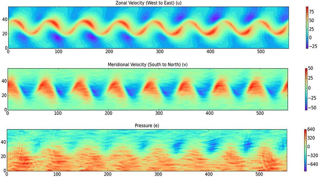
Figure 1. Instances of the zonal (west-east) velocity field, the meridional (south-north) velocity field, and the pressure field, for the SRSW model, after 200 time steps. The distance between any two grid points in both x and y direction is 50 km.

FIGURE 2

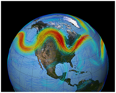
Figure 2. Example of the Jetstream, from NASA at https://svs.gsfc.nasa.gov/3864.

Contributions of the paper

This work is part of the current efforts geared toward developing efficient particle filter methodologies for high-dimensional models originating in (stochastic) geophysical fluid dynamics—see Cotter et al. [10] for a similar application to a stochastic incompressible 2D Euler model with damping and forcing and Cotter et al. [14] for an application to a two-layer quasi-geostrophic model. We study the applicability of such a particle filter methodology based on adaptive tempering and sample regeneration using a Metropolis-Hastings procedure (jittering) to the new SALT-SRSW model (Equation 9) with up to O(10⁴) degrees of freedom. The deterministic rotating shallow water equations are known (see e.g., Kalnay [16], Vallis [17], and Zeitlin [18]) for their complex structure which retains key aspects of the oceanic and the atmospheric dynamics, such as potential vorticity and energy conservation, and the existence of gravity waves. At the same time, RSW systems allow for a proper incorporation of the nonlinear interactions, which makes them favorite systems for modeling geophysical turbulence. Nonetheless, real geophysical systems are even more complex, as they are subject to several small-scale unknown influences which are active at subgrid scales and which cannot be represented even when using modern computational methods with fine resolution grids. The aim of the stochastic terms added in Equation (9) as per [19] is to effectively capture a broad class of such small-scale interactions. This stochastic procedure facilitates the design of more realistic models (as they better integrate the small-scale physics) which can be implemented without exponentially increasing the computational cost. Nonetheless, analyzing, discretising and calibrating such a stochastic model and then assimilating data using it, brings forth several technical challenges. We describe below how we successfully overcome these challenges for the SALT-SRSW model introduced in Equation (9):

• Model implementation. Compressible and incompressible flow simulations can be subject to large discretization errors when all the system variables are defined at the same grid points or at the same time levels. More precisely, spurious modes associated with the pressure field can appear when using a collocated mesh due to the intrinsic structure of the difference scheme which generates an odd-even decoupling between pressure and velocity. To cope with the problem, we use a staggered Arakawa C-grid in which the velocity components are staggered compared to the pressure term i.e., the pressure is stored in the center of the cell, while the velocity components are stored at the cell faces. This generates a reduction of the dispersion errors as well as improvements in the accuracy of the short-wavelength components of the solution⁴. The staggered arrangement, although not easy to implement, is particularly useful in our case as it enables a more accurate implementation of the high-frequency small-scale modes. The system dimension we allow for (i.e., 10⁴) is still far from the dimension of the more realistic models used for example in numerical weather prediction (10¹⁰ and higher).

• Data assimilation. The standard particle filter described above works well for small to medium size models. As the dimension of the model increases, the effectiveness of the standard particle filter diminishes. Heuristically, as the dimension increases so does the distance between the predictive and the posterior distribution. As a result the particles can easily drift away from the truth (there is more space in high dimensions) and will have (possibly exponentially) small likelihoods. In Beskos et al. [7], a new methodology has been proposed to alleviate this problem. The single resampling step in the standard particle filter is replaced by a repeated application of a triple procedure: tempering, resampling and jittering, the number of applications being chosen adaptively by taking into account the effective sample size of the intermediate sample. In the language of Beskos et al. [7], the resulting particle filter is proved to be stable in the dimension, in the sense that it does not degenerate as the dimension increases, whilst keeping the number of particles fixed. In this paper, we successfully adopt the above methodology for the stochastic rotating shallow water model. It is also applied to the Lorenz 63 model where, as expected, the improvements over the standard particle filter are minimal.

• Stochastic transport forcing. There exist a variety of methods of introducing stochasticity to model uncertainty. As examples, we Palmer [22], Majda et al. [23], or Buizza et al. [24]. In general, the noise is introduced into the forcing part of the signal process (the prediction step). Here, we follow the Stochastic Advection by Lie Transport (SALT) approach, introduce in Holm [19], where stochasticity is introduced into the advection part of the model equation so that the resulting stochastic system models the uncertain transport behavior. The resulting equation is different: Although the random shift in the Fourier space is implemented similar to Evensen [25], in this new approach the random parameter multiplies the gradient of the solution and it contains also an extra zero-order operator, see Equation (9). This new form of the noise (whose amplitude is modulated by the ${{L}}_i+{{A}}_i$ operators) is meant to describe the (otherwise un-modeled) effect of the small-scale components on the large-scale components of the fluid. It offers a new approach, termed Stochastic Advection by Lie Transport (SALT), to subgrid transport modeling. To the best of our knowledge this is the first implementation of the SALT rotating shallow water model in a data assimilation setting. Numerical implementations and particle filter algorithms for other SALT models (2D Euler, SQG) have been developed in Cotter et al. [9, 26]. Our numerical implementation of the stochastic forcing is equivalent to the one described in Cotter et al. [9] up to an isomorphism. More precisely, if one applies the approach described in Cotter et al. [9] to a periodic domain, then the stochastic vector fields used in Cotter et al. [9] correspond to the Fourier modes of the transport covariance matrix and they form a basis of the underlying space. This basis may be different from the basis chosen in this paper, but an isomorphism can be established between any two orthogonal bases corresponding to the same underlying space.

The following is a summary of the main numerical experiments and findings contained in this paper:

The Stochastic Lorenz '63 model

• Standard scenario: We run the particle filter over 500 time steps using 50 particles, with each time step of size 0.01 s. The initial uncertainty is equal to 1 and both the observation uncertainty and the model error are equal to 0.1. We use one initial ensemble and all three variables of the system are observed every 20 time steps, with one observation at each analysis time. The observation operator is linear.

• For the other scenarios (see Section 3.2) we vary some of the parameters (e.g., initial uncertainty, observation uncertainty) and compare the results with those obtained in the standard scenario. More importantly, we choose a nonlinear observation operator and analyse the cases where not all three variables of the system are observed.

The SRSW model

• Standard scenario: Using 50 particles, we run the particle filter over 50 time steps, with each time step of size 90 s, on a domain of dimension (n, m) = 60 × 556 with 50km spatial resolution. The layer thickness is 10km. The initial uncertainty and the observation uncertainty are both equal to 1 and model error in the height field is equal to 200 m. The system is observed every 10 time steps and we use one observation at each analysis time.

• To simulate the evolution of the atmospheric Jetstream, the model domain corresponds to a strip situated between 30 and 60° north latitude, with east-west periodic boundary conditions and free-slip boundary conditions on the northern and southern domain.

• For the other scenarios (see Section 4.2) we change some of the parameters and compare the results with those obtained in the standard scenario.

In both cases:

• We test the forecast reliability by comparing the forecast root mean square error (RMSE)

$RMS{E}^2=\Vert \widehat{E}x-x^{\star }{\Vert }^2$

with the forecast ensemble spread (ES)

$E{S}^2=\frac{1}{N-1}{\displaystyle \sum _{i=1}^N\Vert x^i-\widehat{E}x{\Vert }^2}$

where

$\widehat{E}x=\frac{1}{N}{\displaystyle \sum _{i=1}^N{x}^i}$

is the estimated ensemble mean and x^⋆ is the truth.

• Using the adaptive tempering particle filter, the numerical results show that although the dimension of the observation is low compared to the degrees of freedom corresponding to the SPDE, there is sufficient information to allow for an accurate approximation of the truth.

2. The algorithm

To address the problem of filter degeneracy we replace the direct resampling from the weighted predictive approximations with a tempering procedure combined with a sample regeneration using a Metropolis-Hastings methodology (jittering). We give below the basics of the two procedures (further details including the theoretical results justify the applicability of the methods can be found in Beskos et al. [7] and Kantas et al. [8]).

The tempering procedure involves an artificial dynamics which is introduced via a sequence of intermediate target distributions between the predictive and posterior distribution. Each intermediate distribution has a characteristic temperature chosen to ensure that a reasonable number of distinct particles survive.

The temperature is chosen adaptively. More precisely, in order to quantify the spread of the weights, we use the effective sample size statistic:

$\begin{array}{ll}ess(\text{w})=\frac{1}{{\displaystyle \sum _{\ell =1}^N{({\overline{w}}^{\ell })}^2}}& (10)\end{array}$

where ${\overline{\text{w}}}^{\ell }$ are the normalized weights of the particles. In other words, ${\overline{\text{w}}}^{\ell }$ are the original weights divided by the sum of all weights. The temperature is decreased until the effective sample size rises above a certain threshold. This will ensure that the ensemble of particles remains sufficiently diverse after applying the resampling procedure. By iterating the procedure, one obtains a sequence of temperatures 0 = ϕ₀ < ϕ₁ < …ϕ_R = 1 so that, at each time the effective sample size remains above the chosen threshold. Once the temperature is (dynamically) chosen, a resampling procedure is applied. The output approximates the sequence of tempered posterior distributions $p_{t_i}={\pi }_{t_i}^0\to {\pi }_{t_i}^1\to \dots \to {\pi }_{t_i}^R$ that gradually make the transition from the predictive distribution p_ti to the posterior distribution π_ti. The intermediate tempered posterior distribution at the r^th tempering step is given by

$\begin{array}{ll}{\pi }_t^r(B)=\frac{{\displaystyle {\int }_B{\left(g_t^{z_t}(x_t)\right)}^{{\varphi }_r}{p}_t(d{x}_t)}}{{\displaystyle {\int }_{{ℝ}^{d_X}}{\left(g_t^{z_t}(x_t)\right)}^{{\varphi }_r}{p}_t(d{x}_t)}}& (11)\end{array}$

for any $B\in ℬ({ℝ}^{d_X})$ with corresponding normalized tempered weights. The ensembles of particles follows the above artificial dynamics. Each intermediate step incorporates a resampling procedure followed by a jittering one. If we denote by $x^r={(x^{\ell ,r})}_{\ell =1}^N$ the positions of the ensemble of particles at the beginning of the intermediate step r = 0, 1, …R, then at the r-step we resample from

$\begin{array}{ll}{\pi }_{t_i}^{r,N}=\frac{{\displaystyle \sum _{\ell =1}^N}{\text{w}}_{t_i}^{r,\ell }({\varphi }_r,\text{x})\delta (x_{t_i}^{\ell })}{{\displaystyle \sum _{\ell =1}^N}{\text{w}}_{t_i}^{r,\ell }({\varphi }_r,\text{x})},& (12)\end{array}$

where ${\text{w}}_{t_i}^{r,\ell }({\varphi }_r,x)={\left(g_{t_i}^{z_{t_i}}(x_{t_i}^{\ell })\right)}^{{\varphi }_r-{\varphi }_{r-1}}$ The corresponding effective sample size of ${\pi }_{t_i}^{r,N}$ is controlled by a suitable choice of the temperature increment ϕ_r − ϕ_r−1.

As it is well known, the resampling procedure⁵ ensures that particles with low weights are replaced with particles with higher weights. Following the resampling, an ensemble of equal-weighted particles is obtained. An artificial predictive step is then applied, through a Metropolis-Hastings procedure (jittering). This increases the spread of the ensemble whilst keeping the approximation asymptiotycally consistent.

The following is a brief algorithmic description of the tempering and jittering methodology (see also Kantas et al. [8] and Cotter et al. [9]):

1. Initialization: At initial time t = 0: sample N particles from the prior distribution of the signal.

2. Iteration: For any arbitrary time interval (t_i−1, t_i], we start with an ensemble x of N particles with positions ${(x_{t_{i-1}}^{\ell })}_{\ell }$ and we want to assimilate the new observational data z_ti in order to obtain a new ensemble ${(x_{t_i}^{\ell })}_{\ell }$ that defines the approximation ${\pi }_{t_i}^N$ of π_ti. For this we implement the following steps:

2.1. Evolve $x_{t_{i-1}}^{\ell }\underset{\begin{array}{c}SRSW,Lorenz63\end{array}}{\overset{SPDE}{\to }}{x}_{t_i}^{\ell }$.

2.2. Set temperature ϕ = 1.

2.3. While ess_i(ϕ, x) < N_threshold do

∗ Find ϕ′ ∈ (1 − ϕ, 1) such that $es{s}_i({\varphi }^{\prime }-(1-\varphi )),x)\approx N_{threshold}$. Resample according to ${\text{w}}_{t_i}^{\ell }({\varphi }^{\prime }-(1-\varphi )),x)$ and apply MCMC with jittering if required (i.e., if there are duplicates) ⇒ a new ensemble x(ϕ′).

∗ Set ϕ = 1 − ϕ′ and x = x(ϕ).

2.4. If ess_i ≥ N_threshold then go to the (i+1)^th filtering step with ${(x_{t_i}^{\ell },{\text{w}}_i^{\ell })}_{\ell }$.

The Metropolis-Hastings step (jittering) procedure is standard (see, e.g., Cotter et al. [9]), however we will briefly explain the gist of the method. Before applying the method, we have $x_{t_2}^{\ell }={M}(x_{t_1}^{\ell })$ In both models treated below $x_{t_2}^{\ell }$ is an approximation of the solution of a stochastic differential equation that starts from $x_{t_1}^{\ell }$ and it is driven by a Brownian motion W^ℓ. The evolution $x_{t_2}^{\ell }={M}(x_{t_1}^{\ell })$ can then be written as

$x_{t_2}^{\ell }=ℳ(x_{t_1}^{\ell },W^{\ell }(t_1:t_2)),$

where $W^{\ell }(t_1:t_2)$ denotes the Brownian path between t₁ and t₂. In this case the approximation for the predictive distribution is given by

$\begin{array}{ll}{p}_{t_2}=\frac{1}{N}{\displaystyle \sum _{\ell =1}^N}\delta (x_{t_2}^{\ell }).& (13)\end{array}$

As explained above, after each tempering step we resample from the population of particles. As a result, some of the particles end up in the same place. To avoid a large number of duplicates, we apply a Metropolis-Hastings procedure. The proposal for the new position of the particle is obtained by modifying the last part of the particle trajectory. More precisely, we choose

$\begin{array}{ll}{\tilde{x}}_{t_2}^{\ell }={ℳ}_{t_2}\left(x_{t_1}^{\ell },\rho W^{\ell }(t_1:t_2)+\sqrt{1-{\rho }^2}{Z}^{\ell }(t_1:t_2)\right)& (14)\end{array}$

where Z^ℓ is a new standard Brownian motion independent of W^ℓ and ρ is the jittering parameter which controls the size of the perturbation. We found that a suitable choice for ρ is 0.999999 for SALT-SRSW and 0.99 for L63. This is because, in some sense, the particles are already “in the right place” following the resampling step and we wish to move them only ever so slightly. The new position of the particle is accepted with probability $\min \left(1,\frac{{\left(g_{t_i}^{z_{t_i}}({\tilde{x}}_{t_i}^{\ell })\right)}^{{\varphi }_r}}{{\left(g_{t_i}^{z_{t_i}}(x_{t_i}^{\ell })\right)}^{{\varphi }_r}}\right)$ if we are at the r-th intermediate step.

The computational effort C required for each individual assimilation cycle can be estimated as follows: if N is the number of particles, T is the number of tempering steps and J is the number of jittering steps, then C = 0.1 × NJT, where 0.1 × N is the number of duplicates after resampling. In our case, N = 50 and T and J are chosen adaptively (depending on the effective sample size of the ensemble, with the threshold chosen to be 0.8 × N).

3. Applications for the Lorenz 1963 model

3.1. Model description

The Lorenz '63 model is a classical nonlinear three-dimensional model that is a precursor of turbulence theory which has been introduced in Lorenz [27]. It reads

$\begin{array}{ll}\frac{dx}{dt}=\alpha (y-x)& (\mathrm{15a})\end{array}$

$\begin{array}{ll}\frac{dy}{dt}=(\beta -z)x-y& (\mathrm{15b})\end{array}$

$\begin{array}{ll}\frac{dz}{dt}=xy-\gamma z,& (\mathrm{15c})\end{array}$

where α, β, γ are real positive parameters. The model is well-known for the broad spectrum of patterns displayed for different values of α, β, γ and its well-known butterfly attractor. The original values chosen by Lorenz in Lorenz [27] were α = 10, β = 28 and $\gamma =\frac{8}{3}$. For a discussion on the behavior of the solutions for different parameter values see e.g., Sparrow [28]. This model is implemented using a Runge-Kutta scheme of order 4, with initial conditions x₀ = 1.508870, y₀ = −1.531271, z₀ = 25.46091. The details of the Runge-Kutta scheme can be found in Appendix. We perturb the Lorenz '63 model with additive noise: after applying the Runge-Kutta scheme to implement the three variables from system (Equation 15), we generate a Gaussian random field and perturb the system in a manner which is similar to the one explained in Equation (14) to obtain a discrete-time dynamical system that is an approximation of the following system of SDEs, driven by the 3-dimensional Brownian motion W = (W¹, W², W³):

$\begin{array}{ll}dx=\alpha (y-x)dt+\zeta d{W}_t^1& (\mathrm{16a})\end{array}$

$\begin{array}{ll}dy=\left[(\beta -z)x-y\right]dt+\zeta d{W}_t^2& (\mathrm{16b})\end{array}$

$\begin{array}{ll}dz=\left[xy-\gamma z\right]dt+\zeta d{W}_t^3& (\mathrm{16c})\end{array}$

where ζ = 0.1 is the model error.

3.2. Data assimilation results

We perform the data assimilation analysis using an ensemble of 50 particles which we evolve over 500 time steps and each time step has size 0.01. In the standard scenario (Figures 5A–6B) all three variables of the system are observed every 20 time steps. The initial uncertainty is equal to 1, while the observational uncertainty and the model error are equal to 0.1. The jittering parameter ρ is equal to 0.99 in the MCMC step. We present below a couple of scenarios obtained for different values of these parameters. The output is displayed for the first and the third variable. The ensemble of particles is represented through a one standard deviation region around the ensemble mean. We illustrate bellow in Figures 3A,B how the model evolves without any assimilation of data.

FIGURE 3

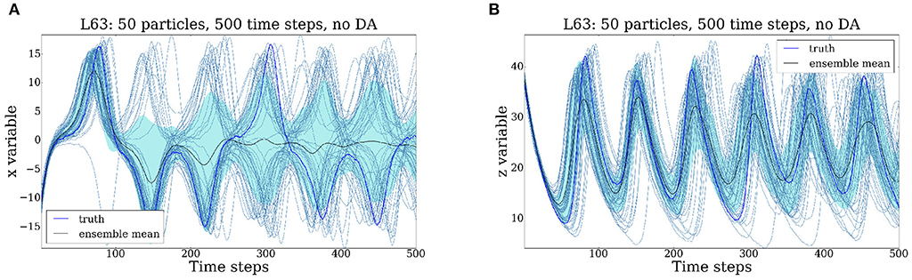
Figure 3. Evolution of the Lorenz '63 model for 500 time steps without any data assimilation. (A) x variable. (B) z variable.

As it can be seen in Figures 3A,B, in the absence of the data assimilation step, the particles spread gradually over the entire attractor. This behavior is exhibited when plotting both the first variable x and the third variable z. In other words, the uncertainty increases (at times quite dramatically). The root mean square error (RMSE) and the ensemble spread (ES) is plotted in Figure 4. In this case the RMSE and the ES oscillate around a value which is comparable with the size of the attractor (in other words, the particles fill out the attractor).

FIGURE 4

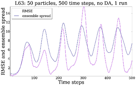
Figure 4. RMSE and ES.

Compared to the previous scenario, we show in Figures 5A–6B that by assimilating observations every 20 time steps, we manage to substantially reduce the uncertainty. Through a repeated application of the forecast/data assimilation step, the cloud of particles successfully tracks the truth which evolves around the attractor set.

FIGURE 5

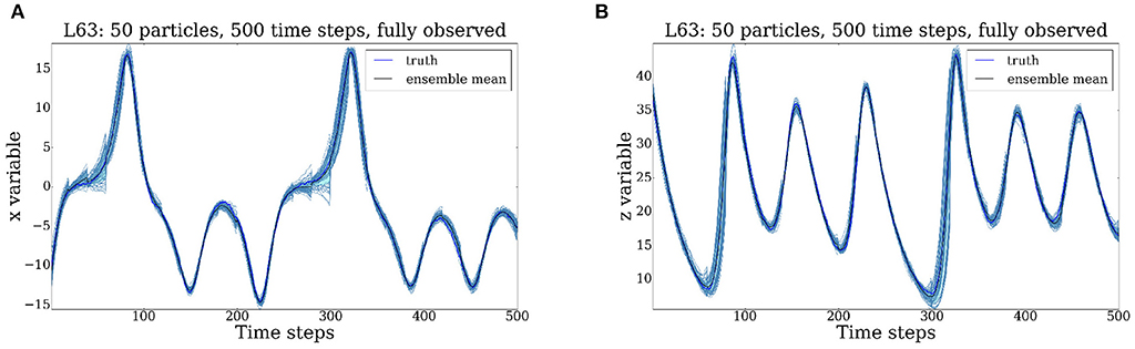
Figure 5. Evolution of the Lorenz '63 model for 500 time steps, all 3 variables are observed every 20 time steps. The initial uncertainty and the observational uncertainty are both equal to 1, the model error is equal to 0.1. Uncertainty is substantially reduced at assimilation times. (A) x variable. (B) z variable.

FIGURE 6

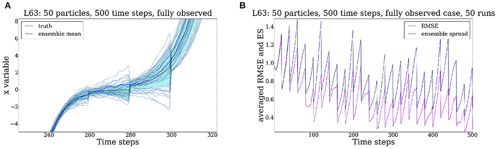
Figure 6. Evolution of the Lorenz '63 model for 500 time steps, all 3 variables are observed every 20 time steps. The initial uncertainty and the observational uncertainty are both equal to 1, the model error is equal to 0.1. Uncertainty is substantially reduced at assimilation times. (A) x variable enlarged. (B) RMSE and ES.

In Figure 6A we exhibit the first three instances to emphasize the reduction of uncertainty resulting from the application of the particle filter with tempering and jittering, as described in Section 1.

We plot in Figure 6B the RMSE and the ES. We can see that the RMSE and the ES are comparable. This is a feature highly appreciated by data assimilation practitioners and e.g., risk managers because it shows that our estimate of the uncertainty as measured by the width of the ensemble is a good estimate of the actual error in the ensemble mean. Based on this measure of success we can conclude that the particle filter performs satisfactory in the case where all the three variables of the system are observed.

In all previous settings the observation operator was linear. We next present the results of two tests (Figures 7A–8D) with nonlinear observation operators. We first make the observations fully nonlinear (Figures 7A–D). More precisely, for these tests the observation operator is chosen to be

$\mathscr{H}(x,y,z)=(x^2,y^2,z^2)$

FIGURE 7

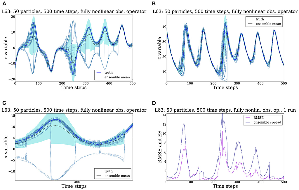
Figure 7. Evolution of the Lorenz '63 model for 500 time steps, all 3 variables are observed every 20 time steps. Observations are denoted by z₁, z₂, z₃. Fully nonlinear observation operator i.e., $z_1=x^2,z_2=y^2,z_3=z^2$ plus noise. (A) x variable. (B) z variable. (C) x variable enlarged. (D) RMSE and ES.

FIGURE 8

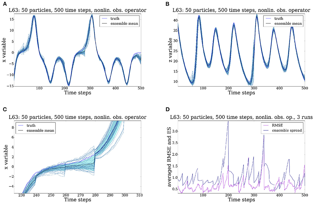
Figure 8. Evolution of the Lorenz '63 model for 500 time steps, all 3 variables are observed every 20 time steps. Observations are denoted by z₁, z₂, z₃. Partially nonlinear observation operator i.e., $z_1=x^2,z_2=y,z_3=z$ plus noise. (A) x variable. (B) z variable. (C) x variable enlarged. (D) RMSE and ES.

with observations given by

$Z={H}(X_t)+V_t$

as explained in Section 1. As we can see from Figure 7A the information available is sufficient to keep the posterior of the third variable concentrated around the truth at all times. However, because of their quadratic relation to the model variables, the observations cannot tell in which wing of the butterfly the truth is situated. This is visible in the solution for x direction. All particles remain on the attractor, and some jump from one wing of the attractor to the other. The uncertainty in the z direction is much smaller, as the z variable is always positive, and hence only one solution is present at all times for this variable. This can be observed in Figure 7B. The values of the RMSE and the ES are plotted in Figure 7D. We can see that both can become very large, essentially of the order of the support of the diffusion (the attractor), as the particles can spread around the entire attractor. This is not surprising as the RMSE is not a useful measure for a bimodal distribution.

Note that these results do not point to a failure of the particle filter. The exact posterior will also show a bi-modal behavior, and the ensemble of particles keep approximating posterior as they should. Methods based on linearizations, such as Ensemble Kalman Filters, would probably show a cloud of particles between the two wings, thus failing to give a meaningful approximation of the posterior distribution.

For the final test case, we make the observation nonlinear just for the first variable (Figures 8A–D). That is,

$\mathscr{H}(x,y,z)=(x^2,y,z).$

In contrast to the previous case, the particle filter follows the truth much better. Ever though the observation operator is only partially linear, the application of the particle filter results in a massive uncertainty reduction. The cloud of particles remains concentrated around the truth and the repeated application of the data assimilation steps keeps the uncertainty in check. Both the x and the z variable (Figures 8A,B) are successfully tracked, as highlighted in Figure 8C. The RMSE and the ES plotted in Figure 8D confirm our findings: most of the time, the RMSE remains in the interval [0, 1] with rare excursions away from this interval. The ensemble spread also remains small, with some oscillations around the assimilation time. The underlying reason for this behavior is that, in this case the system knows in which wing the truth resides via the linear y observation.

4. Applications for the stochastic rotating shallow water model

4.1. Model description

The rotating shallow water model (RSW) is a classical nonlinear fluid dynamics model which contains key aspects of the oceanic and atmospheric dynamics. A detailed analytical description of this model has been provided in Crisan and Lang [1]. From a numerical perspective, the system raises several challenges generated especially by the nonlinear advective terms. Nonlinear advection is a dispersive process. While in a linear inviscid case the wave-like solutions have constant amplitude and propagate at constant speed, in the nonlinear setting wave speeds depend on the wave amplitude, and nonlinear interactions among the waves changes wave amplitudes. The short waves can be amplified by the nonlinear structure, with direct impact on the accuracy of the solution [20]. These intricacies can be overcome by making use of the natural dominant balances which appear in atmosphere and oceans (geostrophic and hydrostatic balance) and by implementing the models using suitable numerical schemes.

The stochastic rotating shallow water model used in our work is given by Equation (9) which in Itô form reads:

$\begin{array}{l}d{v}_t+[u_t·\nabla v_t+f\widehat{z}\times u_t+\nabla p_t]dt\\ +{\displaystyle \sum _{i=1}^{\infty }[({ℒ}_i+{{A}}_i)v_t]d{W}_t^i=\frac{1}{2}}{\displaystyle \sum _{i=1}^{\infty }[{({ℒ}_i+{{A}}_i)}^2{v}_t]dt}& (\mathrm{17a})\end{array}$

$\begin{array}{ll}d{h}_t+\nabla ·(h_t{u}_t)dt+{\displaystyle \sum _{i=1}^{\infty }\left[{ℒ}_i{h}_t\right]d{W}_t^i=\frac{1}{2}}{\displaystyle \sum _{i=1}^{\infty }\left[{ℒ}_i^2{h}_t\right]}dt.& (\mathrm{17b})\end{array}$

The SALT-SRSW model (Equation 17) corresponds to a large-scale stochastic representation of a simplified atmospheric dynamics. The numerical implementation of this system requires to work on a grid of finite resolution and to introduce some sub-grid diffusion terms in order to prevent the accumulation of enstrophy at small scales possibly generated by (direct and inverse) cascading effects. To ensure this, numerical dissipation is artificially introduced by a viscosity term νΔv in the momentum equation. The model (Equation 9) are discretized as described in the Appendix. In the spatial domain, a staggered grid, the Arakawa C-grid, is used because of the low dispersion errors and the lack of computational modes associated with it ([29], pp. 313). A Runge-Kutta scheme of order 4 is used in the time domain. We choose free-slip boundary conditions in the north-south direction and periodic boundary conditions in the east-west direction, on a domain which corresponds to a strip situated between 30 and 60° north latitude. This choice is a consequence of the fact that the model is meant to simulate the evolution of the atmospheric Jetstream, which is maintained by a meridional (south to north) pressure gradient. Hence, the model cannot be periodic in the north-south direction as the pressure in the north has to be smaller than the pressure in the south. Furthermore, the Coriolis parameter is an increasing function of latitude. The free-slip boundary condition ensures that the meridional velocity and the meridional gradient of the zonal velocity are zero, but not the zonal velocity itself.

The model is initialized in so-called geostrophic balance, in which the Coriolis force balances the pressure gradient and all other terms are assumed to be of much smaller magnitude. To this end we prescribe the pressure field as a wave-like field with zonal wave number 8 and calculate the corresponding initial velocity vector field $v_0=(v_0^1,v_0^2)$ using the geostrophic balance condition.

Intuitively, the geostrophic balance can be explained as follows (see e.g., Vallis [30], pp. 58). The large temperature gradient between the north pole and the equator generates a north-south pressure gradient. This pressure gradient will accelerate air parcels toward the north pole. However, as soon as the air parcels are set in motion the Coriolis force starts acting on them, deflecting them to the right (see Equation 9). This eastward deflection continues until the parcels flow due East, and the pressure gradient force and the Coriolis force balance.

The resulting direction of the fluid motion is perpendicular on both the Coriolis force and the pressure force. In the atmosphere and oceans this balance tends to be stable, especially away from the boundaries. Small disturbances to it lead to the appearance of gravity waves that try to restore the balance. The geostrophic balance is dominant as the wind and the currents are usually weak in comparison to the speed of the Earth rotation (Vallis [30], pp.59). The Rossby number in our case is small (ϵ ~ 10⁻¹), meaning that the rotation dominates over the advective part and it is mainly balanced by the pressure gradient force (Crisan et al. [29], pp. 86). The horizontal flow is in “near” geostrophic balance, that is in particular “nearly” divergence-free (Vallis [17], pp.95).

We also assume geostrophic balance for the stochastic forcing described in Section 4.1.1, to strongly reduce the generation of artificial gravity waves. We provide explicit formulas for this in the next subsection, Equation(23).

4.1.1. Stochastic transport forcing

In this subsection we discuss the implementation of the stochastic transport forcing. Recall from Equation (17) that the stochastic transport forcing is given by

$\begin{array}{ll}{\displaystyle \sum _{i=1}^{\infty }}{{B}}_{{\xi }_i}{X}_{t}d{W}_t^i=(\sqrt{{Q}}d{W}_t)X_t=:{R}{X}_t& (18)\end{array}$

where ${ℬ}_{{\xi }_i}:{{W}}^{1,2}({𝕋}^2)\to L^2({𝕋}^2)$ is an operator which depends on the vector fields ξ_i. In our case ${{B}}_{{\xi }_i}$ is equal to ${{L}}_i$ for the forcing applied the depth variable, respectively, it is equal to ${{L}}_i+{{A}}_i$ for the forcing applied to the velocity variable. We interpret ${R}$X_t as a random operator in the following manner. We define the cylindrical Brownian motion

$\sqrt{{Q}}W:={\displaystyle \sum _{i=1}^{\infty }{\xi }_i{W}^i}$

where $\sqrt{{Q}}$ is the corresponding covariance matrix and re-write ${\displaystyle \sum _{i=1}^{\infty }{ℬ}_{{\xi }_i}d{W}_t^i}$ as a random operator applied to the state vector X and we denote it by ${R}$. Here dW is a d-dimensional vector of independent Brownian motions and ${Q}$ is a space-covariance operator. The matrix ${Q}$ has dimension (3d)², where d is the number of mesh points in the space discretisation of (u, v, p). In our case d = 60 × 556 and X_t = (u_t, v_t, p_t). We rewrite (Equation 18) as $(\sqrt{{Q}}dW)\nabla X_t$ for the forcing applied the depth variable, respectively, as $(\sqrt{{Q}}dW)\nabla X_t+\nabla (\sqrt{{Q}}dW)·X_t$ for the forcing applied to the velocity variable.

Once we discretize the SPDE in time and space, the time increments of the cylindrical Brownian motion are replaced by Gaussian random variables with a covariance matrix, which we denote, by a slight abuse of notation, again with ${Q}$.

Given the fact that generating $\sqrt{{Q}}dW$ is computationally expensive for large d, we first do this in the spectral space, and then return to the physical space. The covariance matrix is symmetric and circulant. Using the fast Fourier transform we determine it in the spectral space for a system which is periodic in both the x and y directions. Since our original domain is not periodic, we then truncate the resulting field to the physical domain, in order to avoid a periodic random field. In particular, we compute the Fourier transform of a column corresponding to the circulant matrix. This column has a Gaussian correlation structure. At every time step, we generate a Gaussian random field (again in the spectral space) and then perform the multiplication between the column of the covariance matrix and this newly generated random field. Finally, we use the inverse fast Fourier transform to return to the physical domain.

It is known (see Ruan and McLaughlin [31]) that any continuous random field R can be expressed as a Fourier-Stieltjes integral over a complex-valued Fourier increment dY_R

$\begin{array}{ll}R(\nu )={\displaystyle \int e^{i\mu .\nu }}d{Y}_R(\mu ).& (19)\end{array}$

Therefore, the key ingredient in generating the random field R is the accurate retrieval of the process Y_R(μ). In practice this should be effectuated in discrete space, so that one can compute the integral (Equation 19) numerically. One way of efficiently performing this is by using a complex-valued spectral decomposition, as suggested in Evensen [25]. Let us give details below: The vector fields R can also be expressed as

$\begin{array}{l}R(\nu )=R((x_1,y_1),(x_2,y_2),\dots ,(x_d,y_d))\\ =({\displaystyle {\int }_{{ℝ}^2}{e}^{i{\mu }_1·{\nu }_1}\widehat{R}({\mu }_1)d{\mu }_1,}{\displaystyle {\int }_{{ℝ}^2}{e}^{i{\mu }_2·{\nu }_2}\widehat{R}({\mu }_2)d{\mu }_2,\dots ,}\\ {\displaystyle {\int }_{{ℝ}^2}{e}^{i{\mu }_d·{\nu }_d}\widehat{R}({\mu }_d)d{\mu }_d})& (20)\end{array}$

where $\widehat{R}$ is the Fourier transform of R. In Equation (20) ν = (ν₁, ν₂, …, ν_d) and each ν_i = (x_j, y_ℓ) denotes the variable in the physical space while μ = (μ₁, μ₂, …, μ_d) and ${\mu }_i=({\widehat{x}}_j,{ŷ}_{\ell })$ denotes the corresponding variable in the Fourier space, with j∈{1, …, 60}, ℓ ∈ {1, …, 556}, d ∈ {1, …d} in both cases. Following Evensen [25], for any grid point (x_k1, y_k2) we can write

$\begin{array}{ll}R(x_{k_1},y_{k_2})=\frac{{(2\pi )}^2}{nm\Delta x\Delta y}{\displaystyle \sum _{j,k}\widehat{R}({\widehat{x}}_j,{\widehat{y}}_k)e^{i({\widehat{x}}_j{x}_{k_1}+{\widehat{y}}_k{y}_{k_2})}}& (21)\end{array}$

with x_k1 = k₁Δx, y_k2 = k₂Δy,Δx = x_k1+1 − x_k1, Δy = y_k2+1 − y_k2, ${\widehat{x}}_j=\frac{2\pi j}{n\Delta x}$, ${\widehat{y}}_k=\frac{2\pi k}{m\Delta y}$, and

$\begin{array}{ll}\widehat{R}({\widehat{x}}_j,{\widehat{y}}_k)=\frac{C\sqrt{nm\Delta x\Delta y}}{2\pi }{e}^{-\frac{{\widehat{x}}_j^2+{\widehat{y}}_k^2}{{\sigma }^2}+2\pi i{\phi }_{jk}}.& (22)\end{array}$

where (n, m) = (60, 556) is the dimension of the grid, C corresponds to the amplitude of the random forcing⁶, and φ_jk ∈ [0, 1] is a random number which introduces a random phase shift for any given wave number (as per [25]). Note that R is normally distributed. As mentioned in the previous section, we assume that the dominant balance for the random vectors in this system is the geostrophic balance, that is the pressure gradient force and the Coriolis force balance each other. We have three random vectors: R^v1, R^v2 corresponding to each component of the velocity v = (v¹, v²), and R^p which corresponds to the pressure field p. We obtain them as follows: first, we compute R^p using Equation (21); then we use R^p to compute R^v1 and R^v2 under the geostrophic balance assumption:

$\begin{array}{ll}{R}^{v^1}=-\frac{g}{f}\frac{\partial R^p}{\partial y}& (\mathrm{23a})\end{array}$

$\begin{array}{ll}{R}^{v^2}=\frac{g}{f}\frac{\partial R^p}{\partial x}.& (\mathrm{23b})\end{array}$

Similar types of SALT noise calibration sampled in the Fourier space have been considered in Resseguier et al. [32, 33].

4.2. Data assimilation results

We perform the data assimilation analysis using an ensemble of 50 particles. We plot the ensemble of particles one standard deviation region about the ensemble mean and compare it with the truth. The truth is a pathwise realization of the SRSW model. We start with the standard setting (Figures 9A–D) and show results for 50 model time steps, with a time step size of 90 s (which corresponds to 1.25 h). We use one observation at each analysis time, and the observational uncertainty and the initial uncertainty are equal to 1. The stochastic model error is set to 200 m. As mentioned, the random forcing is implemented using a stochastic advection velocity in SALT. We generate these stochastic advection fields by first generating a stochastic pressure field of standard deviation 200 m, then determining the velocity fields in the zonal and meridional directions using geostrophic balance, as explained in the previous section. These then form the stochastic fields that are applied in all three evolution equations.

FIGURE 9

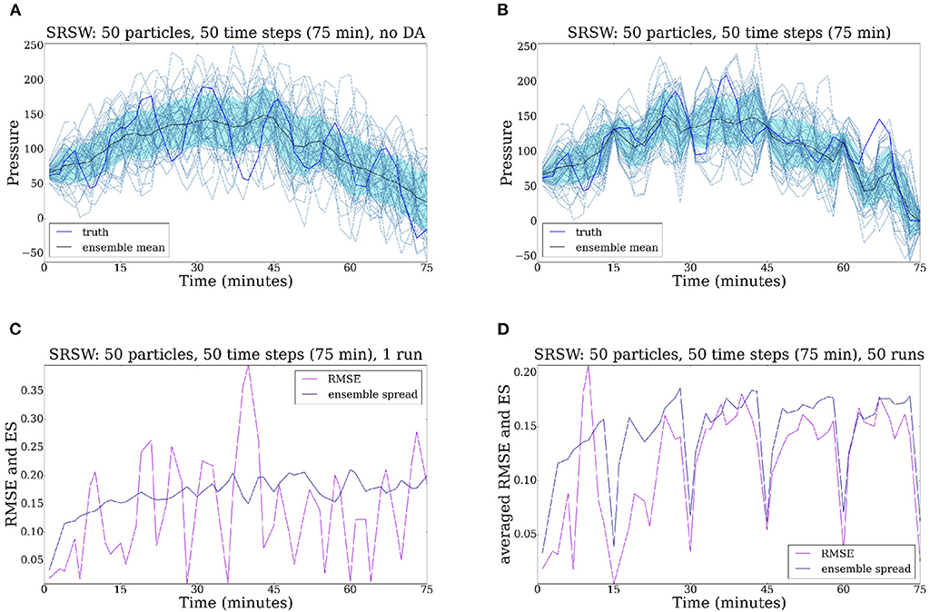
Figure 9. Evolution of the SRSW model for 50 time steps. Left: no assimilation of data. Right: the system is observed every 10 time steps. (A) Pressure field, no DA. (B) Pressure field. (C) RMSE, no DA. (D) RMSE.

We first show the output obtained when no data is assimilated. Figure 9A contains the evolution of the ensemble of particles corresponding to the pressure field at a grid point in the middle of the domain. We can see that the prior distribution is spread out and the truth is not successfully tracked (the ensemble mean remains far from the truth). The ensemble spread is of the same order of the RMSE, showing that the ensemble is consistent.

Now we start to observe the system every 10 time steps (Figures 9B–D), so every 15 min. In Figure 9B one can see that the assimilation of data improves the performance of the ensemble of particles: the standard deviation is reduced and the particle trajectories are corrected at assimilation times. We then decrease the stochastic model error to 50 and observe the system every 5 time steps (Figures 10A,B). In Figure 10A one can notice that the particle filter efficiency is significantly improved by the data assimilation time window: by observing the system more often we obtain a cloud of particles which are better concentrated around the truth. This success is due also to the fact that we decreased the model error to 50. The RMSE and SE illustrated in Figure 10B are much smaller than before⁷.

FIGURE 10

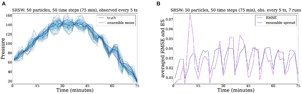
Figure 10. Evolution of the SRSW model for 50 time steps (ts). The system is observed every 5 time steps. The model error is decreased to 50. The particle filter efficacy is improved by the time window and the decreased model error. (A) Pressure field. (B) RMSE.

For the next scenario (Figures 11A,B) the system is observed every 5 time steps and we use 100 observations at each analysis time. Figure 11A shows that a drastic increase in the number of observations (100 now as opposed to 1 as we had before) greatly improves the efficiency of the particle filter. In Figure 11B one can see that the ensemble spread is substantially reduced and the accuracy is now also much better. The true innovation is that although we do not perform any localization, we can assimilate 100 observations without filter degeneracy. This suggest that this particle filter is an important step toward beating the curse of dimensionality that plagued particle filtering for so long.

FIGURE 11

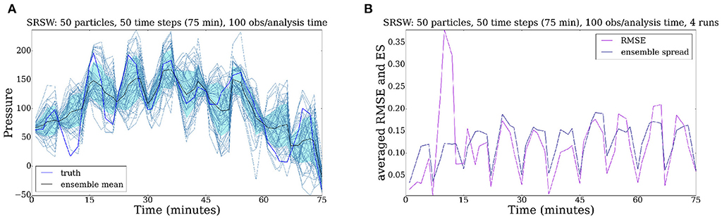
Figure 11. Evolution of the SRSW model for 50 time steps. The system is observed every 5 time steps, with 100 observations/analysis time. A large number of observations improves the performance of the particle filter. (A) Pressure field. (B) RMSE.

We show below (Figures 12A,B) the evolution of the SRSW model for 100 time steps, when observed every 5 time steps, with 5 observations at each analysis time. Although the particles have a constant tendency to diverge from the truth, especially after the first assimilation step, by observing the system quite often and making the observations informative enough, we capture the truth most of the time.

FIGURE 12

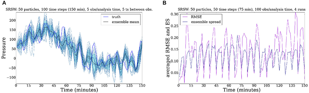
Figure 12. Evolution of the SRSW model for 100 time steps. The system is observed every 5 time steps, with 5 observations/analysis time. The cloud of particles follows the truth most of the time. (A) Pressure field. (B) RMSE.

5. Conclusions and further work

We conclude that our methodology based on a particle filter that incorporates tempering and jittering can be successfully used to assimilate data for both Lorenz '63 and the SALT-SRSW model.

For Lorenz '63 the closeness of the particles to the true evolution of the data assimilation methodology is shown to be influenced by the linearity of the observation operator and the observability of the system. However, when the posterior is wide, e.g., bimodal, the particles should not follow the truth but cover the full posterior distribution, which the tempering particle filter does very well. Three observation operators are used: a fully linear one (${H}$(x, y, z) = (x, y, z)), a partially linear one (${H}$(x, y, z) = (x², y, z)), and a fully nonlinear one (${H}$(x, y, z) = (x², y², z²)). We obtain the best results in the linear case. However, it is worth highlighting that we obtain good results also in the nonlinear case, where we see a bimodal distribution. In contrast to this, a standard Kalman filter would probably fail, due to the difficulties generated by multiple modes. In future research we intend to explore also the influence of other parameters such as: the number of particles, the size of data assimilation window, the effective sample size threshold, the model error.

Moving on to the high-dimensional SRSW case, we conclude that the particle filter remains effective in this case too. We highlight that the particle filter we used in this work does not incorporate any other strategies (such as localization [11, 12]). Following the numerical simulations, the following parameters have a relevant influence on the proficiency of the particle filter:

• DA time window: the results are better when we observe the system every 5 time steps, compared to when we observe it every 10 time steps.

• Number of observations per assimilation time: we test this for 1 observation, 5 observations, and 100 observations, respectively, per analysis time. The best output is obtained in the last case. However, by reducing the number of observations from 100 to 5, but observing the system every 5 time steps, the truth can be well tracked for a long period of time (Figure 12A).

• Model error: the particle filter is shown to be robust with respect to increases in model error.

The experiments show that the system is underobserved, as many real-world systems, such as the atmosphere or the ocean. This is to be expected, as the number of degrees of freedom is very high (~ 100, 080). Nonetheless, the findings in this paper are sufficiently promising to encourage further in-depth investigations based on further improvements in particle filter methodologies. In further work, just as in the case of the Lorenz '63 model, we intend to explore the influence of other parameters such as: the number of particles, observational and initial uncertainty, the effective sample size threshold, variations of the stochastic forcing.

This work constitutes a stepping stone for solving a data assimilation problem where the truth is a model of a horizontal slice of the atmosphere and the data is given by a set of atmospheric pressure observations collected by the German Met Office Deutscher Wetterdienst from pressure sensors carried by commercial aircrafts.

Data availability statement

The original contributions presented in the study are included in the article/Supplementary material, further inquiries can be directed to the corresponding author.

Author contributions

OL contributed to implementing the particle filter and the two stochastic models, running all the numerical tests, adapting the (filtering and jittering) methodology to these two particular cases, and writing up. PL provided a deterministic version of the implementation of the stochastic shallow water model, and contributed to implementing the stochastic forcing, the particle filter with MCMC, and the L63 model. DC contributed by providing the particle filter methodology with tempering and jittering, adapting it to the stochastic shallow water model, proofreading, analysis, and writing up. RP contributed to the analysis and interpretation of the results and proofreading. All authors contributed to the article and approved the submitted version.

Funding

OL and DC were partially supported by the European Research Council (ERC) under the European Union's Horizon 2020 Research and Innovation Programme (ERC, Grant Agreement No. 856408). OL was also partially supported by the EPSRC grant EP/L016613/1 through the Mathematics of Planet Earth Centre for Doctoral Training. PL was supported by the European Research Council (ERC) under the European Union's Horizon 2020 Research and Innovation Programme (ERC, Grant Agreement No. 694509).

Acknowledgments

We would like to thank Wei Pan, Colin Cotter, Darryl Holm, Bertrand Chapron, and Etienne Mmin for many fruitful discussions we had during the preparation of this work.

Conflict of interest

The authors declare that the research was conducted in the absence of any commercial or financial relationships that could be construed as a potential conflict of interest.

Publisher's note

All claims expressed in this article are solely those of the authors and do not necessarily represent those of their affiliated organizations, or those of the publisher, the editors and the reviewers. Any product that may be evaluated in this article, or claim that may be made by its manufacturer, is not guaranteed or endorsed by the publisher.

Supplementary material

The Supplementary Material for this article can be found online at: https://www.frontiersin.org/articles/10.3389/fams.2022.949354/full#supplementary-material

Footnotes

1. ^Note that in Crisan and Lang [1] we work with infinite dimensional function spaces, while here the state space is ${ℝ}^{d_X}$ as we use a grid-based discrete approximation of the solution of Equation (9).

2. ^For a mathematical introduction on the subject, see e.g., Bain and Crisan [2]. For an introduction from the data assimilation perspective of the filtering problem, see van Leeuwen et al. [3] and Reich and Cotter [4].

3. ^Note that in our case b = 0.

4. ^For more details on this type of numerical issues see e.g., Durran [20] or Harlow and Welch [21].

5. ^This is a static procedure.

6. ^In our case C = 1 and we rescale the random vector field R such that it has the desired variance. The parameter ${\sigma }^2=\frac{2}{{10}^2}$ is two times the inverse of a length squared, and it is chosen to specifically determine the spatial covariance length scale of the random field R. For this value of r, the length scale of the random perturbation is 10 grid points.

7. ^Note that all plots are rescaled automatically.

References

1. Crisan D, Lang O. Well-posedness properties for a stochastic rotating shallow water model. arXiv:2107.06601. (2021). doi: 10.48550/arXiv.2107.06601

CrossRef Full Text | Google Scholar

2. Bain A, Crisan, D. Fundamentals of Stochastic Filtering, Vol. 3. New York, NY: Springer (2009).

Google Scholar

3. van Leeuwen PJ, Cheng Y, Reich S. Nonlinear Data Assimilation. Berlin: Springer (2015).

Google Scholar

4. Reich S, Cotter C. Probabilistic Forecasting and Bayesian Data Assimilation. Cambridge: Cambridge University Press (2015).

Google Scholar

5. Vetra-Carvalho S, van Leeuwen PJ, Nerger L, Barth A, Altaf MU, Brasseur P, et al. State-of-the-art stochastic data assimilation methods for high-dimensional non-Gaussian problems. Tellus A. (2018) 70:1445364. doi: 10.1080/16000870.2018.1445364

CrossRef Full Text | Google Scholar

6. van Leeuwen PJ, Künsch HR, Nerger L, Potthast R, Reich S. Particle filters for high-dimensional geoscience applications: a review. Q J R Meteorol Soc. (2019) 145:2335–65. doi: 10.1002/qj.3551

PubMed Abstract | CrossRef Full Text | Google Scholar

7. Beskos A, Crisan D, Jasra, A. On the stability of sequential Monte Carlo methods in high dimensions. Ann Appl Probabil. (2014) 24:4. doi: 10.1214/13-AAP951

CrossRef Full Text | Google Scholar

8. Kantas N, Beskos A, Jasra A. Sequential Monte Carlo methods for high-dimensional inverse problems: a case study for the navier-stokes equations. SIAM/ASA J. (2014) 2:130930964. doi: 10.1137/130930364

CrossRef Full Text | Google Scholar

9. Cotter C, Crisan D, Holm D, Pan W, Shevchenko I. Numerically modelling stochastic Lie transport in fluid dynamics. Multiscale Model Simul. (2019) 17:192–232. doi: 10.1137/18M1167929

CrossRef Full Text | Google Scholar

10. Cotter C, Crisan D, Holm D, Pan W, Shevchenko I. Modelling uncertainty using stochastic transport noise in a 2-layer quasi-geostrophic model. Foundat Data Sci. (2020) 2:2. doi: 10.3934/fods.2020010

CrossRef Full Text | Google Scholar

11. Chen Y, Reich S. Assimilating data into scientific models: an optimal coupling perspective. In: Nonlinear Data Assimilation. Frontiers in Applied Dynamical Systems: Reviews and Tutorials, Vol. 2. Cham: Springer (2015).

12. Potthast R, Walter A, Rhodin A. A localised adaptive particle filter within an operational NWP framework. Mon Weather Rev. (2018) 147:345–62. doi: 10.1175/MWR-D-18-0028.1

CrossRef Full Text | Google Scholar

13. Reich S. Data assimilation: the Schrödinger perspective. Acta Numer. (2019) 28:635–711. doi: 10.1017/S0962492919000011

CrossRef Full Text | Google Scholar

14. Cotter C, Crisan D, Holm D, Pan W, Shevchenko I. Modelling uncertainty using circulation-preserving stochastic transport noise in a 2-layer quasi-geostrophic model. arXiv:1802.05711. (2018).

15. van Leeuwen PJ. Nonlinear data assimilation in geosciences: an extremely efficient particle filter. Q J R Meteorol Soc. (2010) 136:699. doi: 10.1002/qj.699

CrossRef Full Text

16. Kalnay E. Atmospheric Modeling, Data Assimilation and Predictability. Cambridge: Cambridge University Press (2003).

Google Scholar

17. Vallis GK. Atmospheric and Oceanic Fluid Dynamics: Fundamentals and Large-Scale Circulation. 1st ed. Cambridge: Cambridge University Press (2006).

Google Scholar

18. Zeitlin V. Geophysical Fluid Dynamics: Understanding (almost) Everything With Rotating Shallow Water Models. Oxford: Oxford University Press (2018).

Google Scholar

19. Holm D. Variational principles for stochastic fluid dynamics. Proc R Soc A. (2015) 471:20140963. doi: 10.1098/rspa.2014.0963

PubMed Abstract | CrossRef Full Text | Google Scholar

20. Durran DR. Numerical Methods for Fluid Dynamics-With Applications to Geophysics, Second Edition, Vol. 32. New York, NY: Springer. (2010).

Google Scholar

21. Harlow FH, Welch JE. Numerical calculation of time-dependent viscous incompressible flow of fluid with free surface. Phys Fluids. (1965) 8:2182. doi: 10.1063/1.1761178

CrossRef Full Text | Google Scholar

22. Palmer T. The ECMWF ensemble prediction system: looking back (more than) 25 years and projecting forward 25 years. Q J R Meteorol Soc. (2018) 145:12–24. doi: 10.1002/qj.3383

CrossRef Full Text | Google Scholar

23. Majda AJ, Timofeyev I, Eijnden EV. A mathematical framework for stochastic climate models. Commun Pure Appl Math. (2001) 54:891–974. doi: 10.1002/cpa.1014

CrossRef Full Text | Google Scholar

24. Buizza R, Milleer M, Palmer TN. Stochastic representation of model uncertainties in the ECMWF ensemble prediction system. Q J R Meteorol Soc. (1999) 125:2887–908. doi: 10.1002/qj.49712556006

PubMed Abstract | CrossRef Full Text | Google Scholar

25. Evensen G. Sequential data assimilation with a nonlinear quasi-geostrophic model using Monte Carlo methods to forecast error statistics. J Geophys Res. (1994) 99:10,143–10. doi: 10.1029/94JC00572

CrossRef Full Text | Google Scholar

26. Cotter C, Crisan D, Holm D, Pan W, Shevchenko I. A particle filter for stochastic advection by Lie transport (SALT): a case study for the damped and forced incompressible 2D Euler equation. SIAM/ASA J. (2020) 8:1446–92. doi: 10.1137/19M1277606

CrossRef Full Text | Google Scholar

27. Lorenz EN. Deterministic nonperiodic flow. J Atmos Sci. (1963) 20:130–141.

Google Scholar

28. Sparrow C. An introduction to the lorenz equations. IEEE Trans Circ Syst. (1983) Cas-30:8. doi: 10.1109/TCS.1983.1085400

CrossRef Full Text | Google Scholar

29. Crisan D, Holm DD, Cotter C, Cheraghi D, Calderhead B, Broecker J, et al. Mathematics of Planet Earth: A Primer, Advanced Textbooks In Mathematics. London: World Scientific Publishing Europe Ltd. (2017).

30. Vallis GK. Climate and the Oceans. In: Princeton Primers in Climate. Princeton (2012).

Google Scholar

31. Ruan F, McLaughlin D. An efficient multivariate random field generator using the fast Fourier transform. Adv Water Resour. (1998) 21:385–99. doi: 10.1016/S0309-1708(96)00064-4

CrossRef Full Text | Google Scholar

32. Resseguier V, Li L, Jouan G, Drian P, Mmin E, Chapron B. New trends in ensemble forecast strategy: uncertainty quantification for coarse-grid computational fluid dynamics. Arch Comput Methods Eng. (2021) 28:215–61. doi: 10.1007/s11831-020-09437-x

CrossRef Full Text | Google Scholar

33. Resseguier V, Pan W, Fox-Kemper B. Data-driven versus self-similar parameterizations for stochastic advection by Lie transport and location uncertainty. Nonlinear Process Geophys. (2020) 27:209–34. doi: 10.5194/npg-27-209-2020

CrossRef Full Text | Google Scholar