Multipatch stochastic epidemic model for the dynamics of a tick-borne disease

1. Introduction

Tick-borne diseases (TBDs) are progressively affecting human and animal health throughout the world. Ticks transmit pathogens that are responsible for several human and animal diseases such as human monocytic ehrlichiosis (HME), human babesiosis, Lyme disease, Rocky Mountain spotted fever, tick paralysis, anaplasmosis, tick-borne relapsing fever, cowdriosis, and Colorado tick fever [1–3]. Most tick-transmitted pathogens have wildlife species that serve as reservoir hosts [3]. The control, management and prevention of TBDs are difficult because they involve breaking a complex transmission chain between vertebrate hosts and ticks, which interact in a constantly varying environment [3]. HME is a tick-borne zoonotic infection caused by the obligate intracellular bacterium of the genera Ehrlichia [6]. The etiologic agent of HME is Ehrlichia chaffeensis [1–3] and the primary vector of this agent is the lone star tick, Amblyomma americanum [2–4]. Ehrlichia chaffeensis is transmitted to humans through the bite of infected A. americanum [5], and its principal reservoir is believed to be the white-tailed deer, Odocoileus virginianus [1–3, 5] although it is also maintained by a diverse range of wild and domestic animals [6]. The white-tailed deer is preferred by the lone star tick as a key host for blood meals for all its life stages [1–3, 6]. HME was first reported as a human disease in the USA in 1986 [4], with an increasing number of cases being reported to the Center for Disease Control and Prevention [4]. HME is characterized by a moderate-to-severe illness [1] with an estimated fatality rate of 3–5% despite receiving treatment [1].

Spatial spread and persistence of disease depends on the heterogeneity of the landscape, demography and epidemiology of the host [7]. Landscape features such as forests, rivers and roads may result in the separation of populations into discrete patches [7]. Disease dynamics occur within each patch while allowing interaction such as migration or colonization between patches [1]. White-tailed deer and the lone star tick migration from one habitat to another is crucial in the spread of HME. Habitat fragmentation has an impact on host populations, which in turn impacts the spatial dynamics of disease risk [8]. Movement can significantly affect the probability of disease persistence in an area [9]. White-tailed deer migrate due to habitat conditions and social pressures that are based on seasonal influences [2, 10]. Migration rates vary regionally and are influenced by habitat characteristics and competition for resources such as food, cover, and mates [10]. Migration may influence local population levels, and as such decisions to control densities, sex ratios and age structures should consider local deer movement [10]. Ticks can only migrate to a new location while attached to a host and areas that are vulnerable to invasion must have suitable habitat, climate and host communities as well as movement of hosts between established tick populations and novel habitat [2]. Ticks are attached to deer for 1–2 weeks solely for a blood meal and unlike the hosts, they move much shorter distances such that their movement maybe negligible [2]. However, since ticks only feed on deer during certain times of the year, migration rates for ticks must be seasonally linked to deer movement [2]. The spread of pathogens that cause TBDs such as HME can be enhanced by deer movement (in search of cover, food, water, mates, and evading predation) from one habitat to another. Thus, deer movement into new habitats may introduce the disease into habitats that were initially free from it.

Mathematical models have been used for many years in studies involving ticks and TBDs to provide a better understanding of the interaction between ticks and their animal host with regard to disease extinction and persistence. Ordinary differential equation (ODE) models [1, 2, 11–13], stochastic epidemic models [particularly continuous-time Markov chain models [3]], agent-based models [14], and remote sensing [15] have provided insight into the population dynamics of ticks and TBDs. Epidemic models involving multiple patches have also been studied. Arino et al. [16] studied multiple species moving across multiple patches in which they assumed that the population size was constant for each species. Gaff and Gross [2], Gaff and Schaefer [1] studied a metapopulation model with multiple patches for a tick-borne disease. Wang and Mulone [17] investigated the dynamics of a two-patch epidemic model that had a single host species. However, investigations that employ stochastic differential equation (SDE) models to address problems relevant to ticks and TBDs are scarce in the literature. The objective of this study is, therefore, to investigate the impact of between-patch migration of white-tailed deer and lone star ticks on the spatial spread of a tick-borne disease (HME) with regard to disease extinction and persistence using an Itô stochastic differential equation model which is formulated based on an underlying deterministic multipatch model. Specifically, we intend to develop a stochastic model (SDE) for the dynamics of HME in a metapopulation and then use it to determine characteristics of HME that deterministic models could not inform, that is, the probability of extinction and the finite-time to disease extinction. The model that will be developed in this study is an extension of the single patch model that was formulated by Maliyoni et al. [3].

Stochastic epidemic models, e.g., SDE models, are often utilized to model dynamics of biological systems and processes that are stochastic in nature. SDEs account for demographic variability over time due to births, deaths, disease transmission, recovery, migration and state transition rates [7, 18]. The variability inherent in the system may result in dynamics that are different from predictions of the analogous ODE model [3, 7, 19]. Stochastic models provide information about the distribution of extinction time of an epidemic, the total size distribution and the probability of occurrence of an epidemic [18–20]. SDEs are easier to solve using numerical methods than the Kolmogorov differential equations and faster than simulating sample paths of continuous-time Markov chain models [21]. Several studies have also used SDE models to address questions pertinent to epidemiology. For instance, Allen and Victory [22] used an SDE model to account for the random behavior for a schistosomiasis infection that involves human and intermediate snail hosts as well as an additional mammalian host and a competitor snail species. Allen et al. [23] developed an SDE model that was used to estimate persistence-time of a population experiencing demographic and environmental variability. McCormack and Allen [7] formulated an SDE multipatch epidemic model to investigate problems related to wildlife disease persistence and extinction. Kirupaharan and Allen [19] derived an SDE model based on an ODE model to investigate the coexistence of multiple pathogen strains with density-dependent mortality in the absence of co-infection and super-infection. Lahodny and Allen [9] used an SDE model to study the probability of a disease outbreak in multipatch epidemic models. Other interesting studies that have also used SDE models to address various biological problems are found in Allen [24].

In the next section, we describe the multipatch ODE model for a tick-borne disease by extending the model by Maliyoni et al. [3]. We show that the disease-free equilibrium exists and is unique. The general formula for the basic reproduction number is computed and its bounds are determined. In Section 3, we derive an Itô SDE model based on the multipatch ODE model. We perform numerical simulations using the Euler-Maruyama method to illustrate the dynamics of the SDE model in Section 4. In Section 5, the findings and their implications for disease control and prevention are summarized and a conclusion is presented. We also present areas for further study to enhance the findings of this paper.

2. ODE multipatch model

In this section, we formulate the multipatch ODE model for a tick-borne disease. We show that the disease-free equilibrium exists and is unique and the general formula for the basic reproduction number is derived using the next generation matrix operator method.

2.1. Model formulation

Maliyoni et al. [3] studied the transmission dynamics of a tick-borne disease, HME, in a single patch. In this paper, we extend that study by assuming random movement of deer and ticks through w distinct patches that are arranged in a sequence such that individuals freely move to the next patch from their current location. Let w be the total number of patches in which the deer and ticks live. We divide the total population of deer and ticks into susceptible and infected classes in each patch. Thus, let D_j(t), Y_j(t), S_j(t) and X_j(t) denote the number of susceptible deer, infected deer, susceptible ticks and infected ticks in patch j, 1 ≤ j ≤ w, at time t, respectively. The total host and tick population size in patch j is given by N_j(t) = D_j(t)+Y_j(t) and V_j(t) = S_j(t)+X_j(t), respectively.

We assume that an individual in patch j can only access patch j+2 by passing through patch j+1. Similarly, an individual in patch j+2 can migrate to patch j by passing through patch j+1. Figure 1 summarizes deer and tick movement between patches that is considered in this study.

FIGURE 1

Figure 1. Deer and ticks movement through w distinct patches arranged in a sequence for the multipatch model.

We also assume that there is no tick to tick or host to host disease transmission, and no recovery and disease-induced mortality for infected individuals in both populations. Further, we assume that disease transmission from infected deer (or tick) to susceptible tick (or deer) occurs during tick feeding only. The total population for deer grows logistically in each patch with carrying capacity K_j. The external death rate for deer is b_j. The tick growth rate, which incorporates the actual birth, survival and host-finding rates, is ${\widehat{\beta }}_j$. The maximum number of ticks per deer in patch j is M_j and external mortality rate for ticks is ${\widehat{b}}_j$. Disease transmission rate from deer to ticks and ticks to deer in patch j is A_j and Â_j, respectively. The second term in all equations of system (1) represents density-dependent death for the classes in patch j.

Movement between patches is modeled by the term m_jk>0 which is defined as the migration (dispersal) rate of susceptible or infected deer and ticks from patch j to patch k, 1 ≤ j ≤ k ≤ w. We assume that the migration rate for both deer and ticks between patches is the same, that is m_jk = m_kj, since ticks mainly move to new locations while attached to their host for a blood meal; as such their movement is dependent on host movement [2]. We assume that there are no births or deaths of individuals during the migration from one patch to another. Dispersal of individuals out of patch j is largest when the patch population has exceeded the carrying capacity [7]. The population in each patch will grow toward the carrying capacity when there is no migration and disease [25]. The dynamics of the model for w patches are depicted in a compartmental diagram in Figure 2. Parameters in the model are summarized in Table 1.

FIGURE 2

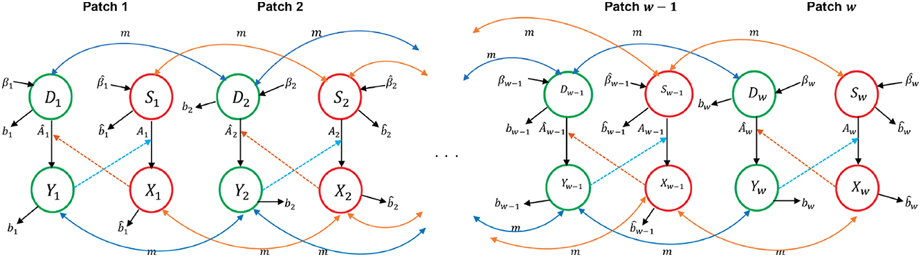
Figure 2. Compartmental flow diagram for the multipatch deer-tick interaction model.

TABLE 1

Table 1. Description of parameters for the multipatch ODE model.

The proposed multipatch deer-tick interaction model satisfies the following system of ODEs:

$\begin{array}{ll}\begin{array}{c}\frac{\text{d}{D}_j}{\text{d}t}={\beta }_j{N}_j-{\beta }_j\frac{D_j{N}_j}{K_j}-{Â}_j\frac{D_j{X}_j}{N_j}-b_j{D}_j+{\displaystyle \sum _{k=1}^w}{m}_{jk}(D_k-D_j),\\ \frac{\text{d}{Y}_j}{\text{d}t}={Â}_j\frac{D_j{X}_j}{N_j}-{\beta }_j\frac{Y_j{N}_j}{K_j}-b_j{Y}_j+{\displaystyle \sum _{k=1}^w}{m}_{jk}(Y_k-Y_j),\\ \frac{\text{d}{S}_j}{\text{d}t}={\widehat{\beta }}_j{V}_j-{\widehat{\beta }}_j\frac{S_j{V}_j}{M_j{N}_j}-A_j\frac{S_j{Y}_j}{N_j}-{\widehat{b}}_j{S}_j+{\displaystyle \sum _{k=1}^w}{m}_{jk}(S_k-S_j),\\ \frac{\text{d}{X}_j}{\text{d}t}=A_j\frac{S_j{Y}_j}{N_j}-{\widehat{\beta }}_j\frac{X_j{V}_j}{M_j{N}_j}-{\widehat{b}}_j{X}_j+{\displaystyle \sum _{k=1}^w}{m}_{jk}(X_k-X_j),\end{array}& (1)\end{array}$

with initial conditions D_j(0) ≥ 0, Y_j(0) ≥ 0, S_j(0) ≥ 0 and X_j(0) ≥ 0 for j = 1, 2, 3, …, w.

The total population size in each patch for host and ticks, respectively, satisfies the following differential equations:

$\begin{array}{ll}\begin{array}{c}\frac{\text{d}{N}_j}{\text{d}t}={\beta }_j{N}_j(1-\frac{N_j}{K_j})-b_j{N}_j+{\displaystyle \sum _{k=1}^w}{m}_{jk}(N_k-N_j),\\ \frac{\text{d}{V}_j}{\text{d}t}={\widehat{\beta }}_j{V}_j(1-\frac{V_j}{M_j{N}_j})-{\widehat{b}}_j{V}_j+{\displaystyle \sum _{k=1}^w}{m}_{jk}(V_k-V_j).\end{array}& (2)\end{array}$

The total population size in all w patches for host, $N(t)=\sum _{j=1}^w{N}_j(t)$, and ticks, $V(t)=\sum _{j=1}^w{V}_j(t)$, satisfy

$\begin{array}{ll}\frac{\text{d}N}{\text{d}t}={\displaystyle \sum _{j=1}^w}\left[{\beta }_j{N}_j(1-\frac{N_j}{K_j})-b_j{N}_j\right]& (3)\end{array}$

and

$\begin{array}{ll}\frac{\text{d}V}{\text{d}t}={\displaystyle \sum _{j=1}^w}\left[{\widehat{\beta }}_j{V}_j(1-\frac{V_j}{M_j{N}_j})-{\widehat{b}}_j{V}_j\right],& (4)\end{array}$

respectively.

In the absence of deer and tick movement between the patches, the system (1) reduces to the model of Maliyoni et al. [3].

2.2. Model properties and equilibria

The variables of system (1) are assumed to be non-negative. For a given set of non-negative initial conditions satisfying N_j(0)>0 and V_j(0)>0, there exists non-negative unique solutions to the multipatch model (1) and all the disease state variables remain non-negative for all time t≥0 [3, 7, 26]. In addition, the total deer and tick populations in the entire metapopulation, N(t) and V(t), respectively, are bounded [26]. Thus, the multipatch model system (1) is mathematically and biologically sensible [26].

2.2.1. Disease-free equilibrium

System (1) has a steady state solution called the disease-free equilibrium (DFE) and satisfies $D_j=D_j^{*}>0$, $S_j=S_j^{*}>0$ and Y_j = X_j = 0 for all j = 1, 2, …, w [26].

Theorem 1. The non-zero DFE for the multipatch model (1) exists and is unique.

Proof . Let Y_j = X_j = 0 for all j = 1, 2, …, w and $D^{*}={(D_1^{*},D_2^{*},\dots ,D_w^{*})}^T$, be the vector of the equilibrium values for susceptible deer. Then from the first equation in system (1), we obtain the following system of equations in matrix form:

$\begin{array}{ll}\left(\begin{array}{cccc}{d}_1+{\displaystyle \sum _{k\ne 1}{m}_{j1}}& -m_{12}& \dots & -m_{1w}\\ -m_{21}& d_2+{\displaystyle \sum _{k\ne 2}{m}_{j2}}& \dots & -m_{2w}\\ ⋮& ⋮& \ddots & ⋮\\ -m_{w1}& -m_{w2}& \dots & d_w+{\displaystyle \sum _{k\ne w}{m}_{kw}}\end{array}\right)\left(\begin{array}{c}{D}_1^{\ast }\\ D_2^{\ast }\\ ⋮\\ D_w^{\ast }\end{array}\right)=\left(\begin{array}{c}{Z}_1\\ Z_2\\ ⋮\\ Z_w\end{array}\right),& (5)\end{array}$

where $d_j=\frac{{\beta }_j{N}_j}{K_j}+b_j$ and Z_j = β_jN_j for all j = 1, 2, …, w.

System (5) can be written as

$\begin{array}{ll}{C}_1{D}^{*}=Z,& (6)\end{array}$

where

$\begin{array}{lll}{C}_1& =& \text{diag}\left(d_j+{\displaystyle \sum _{k=1,k\ne j}^w}{m}_{kj}\right)-M^d,Z={(Z_1,Z_2,\dots ,Z_w)}^T,\end{array}$

$\begin{array}{ll}{M}^d=\left(\begin{array}{cccc}0& m_{12}& \dots & M_{1w}\\ m_{21}& 0& \dots & m_{2w}\\ ⋮& ⋮& \ddots & ⋮\\ m_{w1}& m_{w2}& \dots & 0\end{array}\right).& (7)\end{array}$

Similarly, let $S^{*}={(S_1^{*},S_2^{*},\dots ,S_w^{*})}^T$ be the vector of the equilibrium values for susceptible ticks. We write the third equation in model system (1) as the following system of equations in matrix form:

$\begin{array}{ll}\left(\begin{array}{cccc}{c}_1+{\displaystyle \sum _{k\ne 1}{m}_{j1}}& -m_{12}& \dots & -m_{1w}\\ -m_{21}& c_2+{\displaystyle \sum _{k\ne 2}{m}_{j2}}& \dots & -m_{2w}\\ ⋮& ⋮& \ddots & ⋮\\ -m_{w1}& -m_{w2}& \dots & c_w+{\displaystyle \sum _{k\ne w}{m}_{kw}}\end{array}\right)\left(\begin{array}{c}{S}_1^{\ast }\\ S_2^{\ast }\\ ⋮\\ S_w^{\ast }\end{array}\right)=\left(\begin{array}{c}{L}_1\\ L_2\\ ⋮\\ L_w\end{array}\right),& (8)\end{array}$

where $c_j=\frac{{\widehat{\beta }}_j{V}_j}{M_j{N}_j}+{\widehat{b}}_j$ and $L_j={\widehat{\beta }}_j{V}_j$ for all j = 1, 2, …, w.

We rewrite system (8) as

$\begin{array}{ll}{C}_2{S}^{*}=L,& (9)\end{array}$

where

$C_2=\text{diag}\left(c_j+{\displaystyle \sum _{k=1,k\ne j}^w}{m}_{kj}\right)-M^d$

and $L={(L_1,L_2,\dots ,L_w)}^T$.

The matrix C₁ in Equation (6) has positive column sums and negative off-diagonal entries. Thus, matrix C₁ is an irreducible and non-singular M-matrix [27] and therefore, C₁ must have a positive inverse, that is, $C_1^{-1}>0$. Hence, the equation $D^{*}=C_1^{-1}Z>0$ is the unique solution of the equation $C_1{D}^{*}=Z$ [27]. The analysis of matrix C₂ in Equation (9) is the same as that of matrix C₁ above. Hence, $C_2^{-1}$ exists and is positive. Therefore, $S^{*}=C_2^{-1}L>0$ is the unique solution of the equation $C_2{S}^{*}=L$ [27]. These results show that the DFE always exists and is unique.

2.3. Basic reproduction number

We derive the general formula for the basic reproduction number, ℜ₀ for the multipatch model (1). ℜ₀ is defined as the average number of secondary infections that a single infected individual would produce in a totally susceptible population during the entire duration of infectiousness [28, 29]. Mathematically, ℜ₀ is a threshold quantity that often determines the extinction or persistence of the disease [28]. In general, if ℜ₀ < 1, then the disease dies out in the population and if ℜ₀>1, then the disease may invade the susceptible population and persist [28–30]. We use the method developed by van den Driessche and Watmough [29] to compute ℜ₀.

We order the infected variables in model (1) by disease state and by patch, that is,

$Y_1,Y_2,\dots ,Y_w,X_1,X_2,\dots ,X_w.$

Then, the matrices F and V for the new infection and all remaining transfer terms, respectively, are given by

$\begin{array}{ll}F=\left(\begin{array}{cc}0& F_{12}\\ F_{21}& 0\end{array}\right)\text{and}V=\left(\begin{array}{cc}{V}_{11}& 0\\ 0& V_{22}\end{array}\right),& (10)\end{array}$

with

$\begin{array}{c}{F}_{12}=\text{diag}({\widehat{A}}_j{h}_j);h_j=M_j({\widehat{\beta }}_j-{\widehat{b}}_j)/{\widehat{\beta }}_j),\\ F_{21}=\text{diag}(A_j),\\ V_{11}=\text{diag}\left({\beta }_j+{\displaystyle \sum _{k=1,k\ne j}^w{m}_{jk}}\right)-M^d,\\ V_{22}=\text{diag}\left({\widehat{\beta }}_j+{\displaystyle \sum _{k=1,k\ne j}^w{m}_{jk}}\right)-M^d.\end{array}$

Matrix M^d is defined in Equation (7). The basic reproduction number of model (1) is the spectral radius of matrix FV⁻¹, that is,

$\begin{array}{l}{\Re }_0=\rho (F{V}^{-1})\end{array}$

where

$\begin{array}{ll}F{V}^{-1}\hfill & =\left(\begin{array}{cc}0& F_{12}\\ F_{21}& 0\end{array}\right){\left(\begin{array}{cc}{V}_{11}& 0\\ 0& V_{22}\end{array}\right)}^{-1},\hfill \\ \hfill & =\left(\begin{array}{cc}0& F_{12}{V}_{22}^{-1}\\ F_{21}{V}_{11}^{-1}& 0\end{array}\right).\hfill \end{array}$

Therefore,

$\begin{array}{l}{\Re }_0=\sqrt{F_{21}{V}_{11}^{-1}{F}_{12}{V}_{22}^{-1}}.\end{array}$

Theorem 2 follows from [29, 30].

Theorem 2. If ℜ₀ < 1, then the disease-free equilibrium is locally asymptotically stable and if ℜ₀>1, then it is unstable.

The basic reproduction number depends on the migration rate of the infected deer and ticks whereas the disease-free equilibrium depends on the migration rate of susceptible deer and ticks [7]. The patch reproduction number is defined as the basic reproduction number for an individual patch j = 1, 2, …, w and is given by [7, 9]

$\begin{array}{ll}{\Re }_0^j=\sqrt{\frac{{Â}_j{A}_j{M}_j({\widehat{\beta }}_j-{\widehat{b}}_j)}{{\widehat{\beta }}_j^2{\beta }_j}}.& (11)\end{array}$

If there is no migration of deer and ticks, m_jk = 0 for all j, k, then the basic reproduction number, ℜ₀ is equal to the largest patch reproduction number, ${\Re }_0^j$ [7].

Theorem 3. Let the migration rate m_jk = 0 for j, k = 1, 2, …, w. Then the basic reproduction number, ℜ₀ of the multipatch model (1) is equal to the largest patch reproduction number, ${\Re }_0^j$ [7], that is,

$\begin{array}{ll}{\Re }_0={\displaystyle \underset{1\le j\le w}{max}}\left\{{\Re }_0^j\right\}.& (12)\end{array}$

Proof. Let m_jk = 0. Then matrices F and V in (10) are defined by

$\begin{array}{ll}{F}_{12}\hfill & =\text{diag}({\widehat{A}}_j{h}_j),\hfill \\ F_{21}\hfill & =\text{diag}(A_j),\hfill \\ V_{11}\hfill & =\text{diag}({\beta }_j),\hfill \\ V_{22}\hfill & =\text{diag}({\widehat{\beta }}_j).\hfill \end{array}$

Now,

$\begin{array}{ll}F{V}^{-1}=\left[\begin{array}{cc}0& \text{diag}\left(\frac{{\widehat{A}}_j{h}_j}{{\widehat{\beta }}_j}\right)\\ \text{diag}\left(\frac{A_j}{{\beta }_j}\right)& 0\end{array}\right]& (13)\end{array}$

and hence

$\begin{array}{l}{\Re }_0=\rho (F{V}^{-1})={\Re }_0^j\end{array}$

which satisfies the relationship in Equation (12).

Equation (12) means that when there is no migration, then the reproduction number of the entire patch system is simply the largest reproduction number of the individual patches. Thus, if the largest reproduction number is greater than 1, then even though the reproduction number can be less than 1 in the other patches, the entire patch system will be considered to have an outbreak. But if the largest reproduction number is less than 1, then it means that all other patches have reproduction numbers that are less than 1 and the infection can be regarded to be under control.

Now, if there is migration, that is, m_jk>0, then the bounds given in Theorem 4 can be obtained for ℜ₀ for w patches.

Theorem 4. Let m_jk>0. Then the basic reproduction number, ℜ₀ for the multipatch model (1) satisfies the following inequality [7, 30]:

$\begin{array}{ll}{\displaystyle \underset{1\le j\le w}{min}}\left\{{\Re }_0^j\right\}\le {\Re }_0\le {\displaystyle \underset{1\le j\le w}{max}}\left\{{\Re }_0^j\right\}.& (14)\end{array}$

Theorem 4 means that if migration is allowed, that is, m_jk>0, then the entire patch system reproduction number lies between the reproduction numbers of the patch with the lowest and largest reproduction numbers. In other words, this implies that if the disease cannot be sustained in any of the individual patches in isolation (that is, when migration in not allowed), then it cannot be sustained in the entire patch system when migration from one patch to another is allowed. Further, if the disease can be sustained in every patch of isolated patches and migration in not allowed, then the disease can also be sustained in the entire patch system when the patches are connected and migration from one patch to another is allowed [7].

It is worth noting that if ${\Re }_0^j<1$ for all j, then the disease dies out (see Figure A1 for the numerical illustration of this) while if ${\Re }_0^j>1$ for all j, then the DFE is unstable and the disease may invade the population [30]. If ${\Re }_0^j<1$ in patch j, then the disease dies out in patch j whereas if ${\Re }_0^j>1$ in patch j, then the disease becomes endemic in patch j [9, 30]. When all the w patches are identical, ℜ₀ is equal to ${\Re }_0^j$ and is the same for all patches [7]. If the system is at an equilibrium and one patch is at the DFE (or endemic level), then all patches, j = 1, 2, …, w are at the DFE (or endemic level) [30]. These results hold by assuming that the directed graph determined by the migration rates is strongly connected [30].

3. SDE multipatch model derivation

We now derive a system of Itô SDEs from the multipatch ODE model (1) and the probabilities associated with possible changes given in (18). The derivation follows the procedure described by Allen [24, 31], Kirupaharan and Allen [19] and Allen [18]. The derivation procedure shows the relationship between discrete-time Markov chain and continuous-time Markov chain processes and the derived system of SDEs [18]. The advantage of this procedure is that parameters in the model are better understood since they are derived from basic assumptions [31]. A general procedure for deriving an SDE model from an ODE model is not included in this paper but can be found in [18, 19, 24, 31]. For an SDE, the time and state variables are both continuous [9, 19–21, 32].

Let D_j(t), Y_j(t), S_j(t), and X_j(t) be continuous random variables representing the number of susceptible deer, infected deer, susceptible ticks and infected ticks in patch j, 1 ≤ j ≤ w, respectively, at time t∈[0, ∞). The random variables satisfy N_j(t) = D_j(t)+Y_j(t), V_j(t) = S_j(t)+X_j(t) and D_j(t), Y_j(t), S_j(t), X_j(t)∈[0, ∞). Also, let the random vector H(t) be defined as

$\begin{array}{l}H(t)=[D_1(t),D_2(t),\dots ,D_w(t),Y_1(t),Y_2(t),\dots ,\\ Y_w(t),S_1(t),S_2(t),\dots ,S_w(t),\\ X_1(t),X_2(t),\dots ,X_w(t){]}^T.& (15)\end{array}$

The derivation of the SDE model is based on a Markov chain model with a small time interval, Δt [25]. We assume that in a sufficiently small time Δt, there can be at most one change, ±1, in the random variable H(t) [7, 18, 20, 24]. Let the change in the populations during the time interval Δt be defined by

$\begin{array}{ll}\begin{array}{ccc}\Delta D_j(t)& =& D_j(t+\Delta t)-D_j(t),\\ \Delta Y_j(t)& =& Y_j(t+\Delta t)-Y_j(t),\\ \Delta S_j(t)& =& S_j(t+\Delta t)-S_j(t),\\ \Delta X_j(t)& =& X_j(t+\Delta t)-X_j(t).\end{array}& (16)\end{array}$

Also, let

$\begin{array}{l}\Delta H(t)=[\Delta D_1(t),\dots ,\Delta D_w(t),\Delta Y_1(t),\dots ,\Delta Y_w(t),\\ \Delta S_1(t),\dots ,\Delta S_w(t),\Delta X_1(t),\dots ,\Delta X_w(t){]}^T,& (17)\end{array}$

be the vector for the incremental changes in the population sizes over the interval Δt.

We compute the transition probabilities corresponding to the possible changes for the random variables. It is assumed that probabilities for the possible changes in (18) are proportional to the time interval Δt [24]. The transition probabilities are given by:

$\begin{array}{l}\text{ Prob}\{\Delta D_j=1|H(t)\}={\beta }_j{N}_j\Delta t+o(\Delta t),\\ \text{ Prob}\{\Delta D_j=-1|H(t)\}=({\beta }_j{N}_j/K_j+b_j)D_j\Delta t+o(\Delta t),\\ \text{ Prob}\{\Delta D_j=-1,\Delta Y_j=1|H(t)\}={\widehat{A}}_j{D}_j{X}_j/N_j\Delta t+o(\Delta t),\\ \text{ Prob}\{\Delta D_j=1,\Delta D_k=-1|H(t)\}=m_{kj}{D}_k\Delta t+o(\Delta t),\\ \text{ Prob}\{\Delta D_j=-1,\Delta D_k=1|H(t)\}=m_{jk}{D}_j\Delta t+o(\Delta t),\\ \text{ Prob}\{\Delta Y_j=-1|H(t)\}=({\beta }_j{N}_j/K_j+b_j)Y_j\Delta t+o(\Delta t),\\ \text{ Prob}\{\Delta Y_j=1,\Delta Y_k=-1|H(t)\}=m_{kj}{Y}_k\Delta t+o(\Delta t),\\ \text{ Prob}\{\Delta Y_j=-1,\Delta Y_k=1|H(t)\}=m_{jk}{Y}_j\Delta t+o(\Delta t),\\ \text{ Prob}\{\Delta S_j=1|H(t)\}={\widehat{\beta }}_j{V}_j\Delta t+o(\Delta t),\\ \text{ Prob}\{\Delta S_j=-1|H(t)\}\text{}=\text{}({\widehat{\beta }}_j{V}_j/M_j{N}_j+{\widehat{b}}_j)S_j\Delta t+o(\Delta t),\\ \text{ Prob}\{\Delta S_j=-1,\Delta X_j=1|H(t)\}=A_j{Y}_j{S}_j/N_j\Delta t+o(\Delta t),\\ \text{ Prob}\{\Delta S_j=1,\Delta S_k=-1|H(t)\}=m_{kj}{S}_k\Delta t+o(\Delta t),\\ \text{ Prob}\{\Delta S_j=-1,\Delta S_k=1|H(t)\}=m_{jk}{S}_j\Delta t+o(\Delta t),\\ \text{ Prob}\{\Delta X_j=-1|H(t)\}\text{}=\text{}({\widehat{\beta }}_j{V}_j/M_j{N}_j+{\widehat{b}}_j)X_j\Delta t\text{}+\text{}o(\Delta t),\\ \text{ Prob}\{\Delta X_j=1,\Delta X_k=-1|H(t)\}=m_{kj}{X}_k\Delta t+o(\Delta t),\\ \text{ Prob}\{\Delta X_j=-1,\Delta X_k=1|H(t)\}=m_{jk}{X}_j\Delta t+o(\Delta t).& (18)\end{array}$

We calculate the expected rate of change E[ΔH(t)] and the covariance matrix E[ΔH(t)(ΔH(t))^T] of the population over a short time step Δt based on transition probabilities in (18). Neglecting multiple changes in time Δt which have probabilities of order (Δt)², the expected rate of change to order Δt is a 4w×1 vector given by

$\begin{array}{l}E[\Delta H(t)]=\\ \left(\begin{array}{c}{\beta }_1{N}_1-\left(\frac{{\beta }_1{N}_1}{K_1}+b_1\right)D_1-\frac{{\widehat{A}}_1{D}_1{X}_1}{N_1}+{\displaystyle \sum _{k=1}^w{m}_{1k}}(D_k-D_1)\\ ⋮\\ {\beta }_w{N}_w-\left(\frac{{\beta }_w{N}_w}{K_w}+b_w\right)D_w-\frac{{\widehat{A}}_w{D}_w{X}_w}{N_w}+{\displaystyle \sum _{k=1}^w{m}_{wk}}(D_k-D_w)\\ \frac{{\widehat{A}}_1{D}_1{X}_1}{N_1}-\left(\frac{{\beta }_1{N}_1}{K_1}+b_1\right)Y_1+{\displaystyle \sum _{k=1}^w{m}_{1k}}(Y_k-Y_1)\\ ⋮\\ \frac{{\widehat{A}}_w{D}_w{X}_w}{N_w}-\left(\frac{{\beta }_w{N}_w}{K_w}+b_w\right)Y_w+{\displaystyle \sum _{k=1}^w{m}_{wk}}(Y_k-Y_w)\\ {\widehat{\beta }}_1{V}_1-\left(\frac{{\widehat{\beta }}_1{V}_1}{M_1{N}_1}+{\widehat{b}}_1\right)S_1-\frac{A_1{Y}_1{S}_1}{N_1}+{\displaystyle \sum _{k=1}^w{m}_{1k}}(S_k-S_1)\\ ⋮\\ {\widehat{\beta }}_w{V}_w-\left(\frac{{\widehat{\beta }}_w{V}_w}{M_w{N}_w}+{\widehat{b}}_w\right)S_w-\frac{A_w{Y}_w{S}_w}{N_w}+{\displaystyle \sum _{k=1}^w{m}_{wk}}(S_k-S_w)\\ \frac{A_1{Y}_1{S}_1}{N_1}-\left(\frac{{\widehat{\beta }}_1{V}_1}{M_1{N}_1}+{\widehat{b}}_1\right)X_1+{\displaystyle \sum _{k=1}^w{m}_{1k}}(X_k-X_1)\\ ⋮\\ \frac{A_w{Y}_w{S}_w}{N_w}-\left(\frac{{\widehat{\beta }}_w{V}_w}{M_w{N}_w}+{\widehat{b}}_w\right)X_w+{\displaystyle \sum _{k=1}^w{m}_{wk}}(X_k-X_w)\end{array}\right)\Delta t,\\ =\alpha \Delta t.& (19)\end{array}$

and the covariance matrix to order Δt is a 4w×4w matrix defined by [18, 19, 21, 22, 24, 31]

$\begin{array}{ll}C\left[\Delta H(t)\right]=E\left[\Delta H(t){(\Delta H(t))}^T\right]-E\left[\Delta H(t)\right]{\left[E\left[\Delta H(t)\right]\right]}^T.& (20)\end{array}$

The second term on the right side of Equation (20) is of order (Δt)² and hence the covariance matrix is approximately equal to E[ΔH(t)(ΔH(t))^T] [19, 21, 24, 31], that is,

$\begin{array}{ll}\begin{array}{lll}C[\Delta H(t)]\approx E[\Delta H(t){(\Delta H(t))}^T]\hfill & =\hfill & \left[\begin{array}{ccccccc}B& & E& & 0& & 0\\ E& & H& & 0& & 0\\ 0& & 0& & P& & Q\\ 0& & 0& & Q& & U\end{array}\right]\Delta t,\hfill \\ \hfill & =\hfill & C\Delta t,\hfill \end{array}& (21)\end{array}$

where B, E, H, P, Q, and U are w×w sub-matrices defined by

$\begin{array}{ll}\begin{array}{ll}B\hfill & ={\beta }_j{N}_j+({\beta }_j{N}_j/K_j+b_j)D_j+{\widehat{A}}_j{D}_j{X}_j/N_j+{\displaystyle \sum _{i=1,i\ne j}^w{m}_{ji}}(D_i+D_j),\hfill \\ E\hfill & =\text{diag}(-{\widehat{A}}_j{D}_j{X}_j/N_j),\hfill \\ H\hfill & ={\widehat{A}}_j{D}_j{X}_j/N_j+({\beta }_j{N}_j/K_j+b_j)Y_j+{\displaystyle \sum _{i=1,i\ne j}^w{m}_{ji}}(Y_i+Y_j),\hfill \\ P\hfill & ={\widehat{\beta }}_j{V}_j+({\widehat{\beta }}_j{V}_j/M_j{N}_j+{\widehat{b}}_j)S_j+A_j{Y}_j{S}_j/N_j+{\displaystyle \sum _{i=1,i\ne j}^w{m}_{ji}}(S_i+S_j),\hfill \\ Q\hfill & =\text{diag}(-A_j{Y}_j{S}_j/N_j),\hfill \\ U\hfill & =A_j{Y}_j{S}_j/N_j+({\widehat{\beta }}_j{V}_j/M_j{N}_j+{\widehat{b}}_j)X_j+{\displaystyle \sum _{i=1,i\ne j}^w{m}_{ji}}(X_i+X_j).\hfill \end{array}& (22)\end{array}$

The system of Itô SDEs for the stochastic process is written by obtaining the square root of matrix CΔt or a matrix G (given in Equation A1 in Appendix 3) such that GG^T = C [21, 31, 33]. Each column of matrix G is the square root of the changes and probabilities given in Equation (18) [21]. The covariance matrix C is a symmetric positive definite matrix and therefore, has a unique positive definite square root, $G=\sqrt{C}$ [7, 18, 19, 31]. Assuming that H(t) is sufficiently large in a small interval Δt, then the change ΔH(t) has approximately a normal distribution with mean vector αΔt and covariance matrix CΔt; that is, ΔH(t)~N(αΔt, CΔt) which follows from the Central Limit Theorem [18, 19, 21, 31]. Letting Δt → 0, leads to the system of Itô SDEs [18, 21, 31]

$\begin{array}{ll}\frac{\text{d}H(t)}{\text{d}t}=\alpha (H(t))+G(H(t))\frac{\text{d}W(t)}{\text{d}t},& (23)\end{array}$

where α(H(t)) is the drift vector, G(H(t)) is a diffusion matrix [9, 31] and $W(t)={(W_1(t),\dots ,W_n(t))}^T$ is a vector of n independent Wiener processes [9, 18, 21, 24, 31] with n representing the total number of possible changes of the stochastic process [9]. The Wiener process W_i(t) is a random variable and is normally distributed with mean zero and variance t, W_i(t)~N(0, t) [18, 21, 24, 31, 34]. The system of Itô SDEs (23) reduces to the original ODE model (1), if the terms associated with the independent Wiener processes are dropped [21] or matrix G = 0 [24, 31] in Equation (23). It is assumed that α and G satisfy certain smoothness and growth conditions in the time and state variables that guarantee existence and uniqueness of solutions to Equation (23) [19, 24, 35] as indicated in Theorem 5:

Theorem 5. Let α(P) and G(P) be functions satisfying the Lipschitz continuity and linear growth conditions. In other words, there exists constants g₁>0 and g₂>0 such that for all t∈[0, T] and P, Q∈ℝⁿ, the following conditions hold

a) |α(P) − α(Q)|+|G(P) − G(Q)| ≤ g₁|P − Q| (Lipschitz continuity).

b) |α(P)| + |G(P)| ≤ g₂(1 + |P|) (Linear growth).

Then, the stochastic differential equation

$\begin{array}{ll}dH(t)=\alpha (H(t))\text{d}t+G(H(t))\text{d}W(t),0\le t\le T& (24)\end{array}$

has a pathwise unique, t-continuous solution H(t) with the property that

$\begin{array}{l}{\displaystyle \underset{0\le t\le T}{sup}}E\left[|H(t){|}^2\right]<\infty ,\end{array}$

where E is the expectation [18, 34, 36].

Conditions (a) and (b) in Theorem 5 ensure that solutions H(t) do not become infinite in finite time and are pathwise unique, respectively [18]. The proof for Theorem 5 can be found in Kloeden and Platen [36] and Øksendal [34].

4. Numerical simulations

In this section, we illustrate the dynamics of the multipatch ODE and SDE models for deer and ticks. We consider an example of a two-patch model and apply the Euler-Maruyama numerical method to approximate sample paths of the SDE model. Further, we vary the migration rate between the two patches in order to investigate the impact of migration on disease extinction and persistence. The patch parameter values used in the numerical simulations are given in Table 2 and all the results in this section are based on those parameter values. The explicit system of the two-patch ODE and SDE models is given in Appendices 2, 3, respectively.

TABLE 2

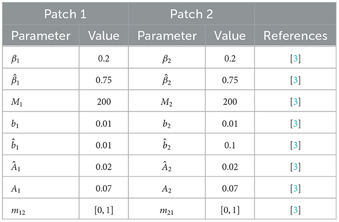
Table 2. Patch parameter values for the two-patch ODE and SDE models. All rates are per month.

In this paper, we have assumed that the migration rate from patch 1 to patch 2 and vice versa is the same; as such we use m for migration rate instead of m₂₁ and m₁₂ as indicated in Table 2. The patch reproduction numbers for patch 1 and patch 2 are ${\Re }_0^1=1.3571$ and ${\Re }_0^2=1.2719$, respectively. For m = 0 (isolated patches), the basic reproduction number is equal to the largest patch reproduction number, that is, ${\Re }_0={\Re }_0^1=1.3571$ (see Theorem 3). For m>0 (connected patches), the basic reproduction number lies between the minimum and the maximum of the two patch reproduction numbers; 1.2719 ≤ ℜ₀ ≤ 1.3571 (see Theorem 4).

Figure 3 shows the solution of the ODE model and one sample path of the SDE model for the two patches in isolation (m = 0). The number of infected deer and ticks increases before stabilizing in both patches but the rate of the increase is higher in patch 1 than in patch 2. Thus, the disease invades the susceptible deer and tick population and persists in both patches for the ODE model. Eventually, the population in both patches approaches the stable endemic equilibrium (see Table 3). since the basic reproduction number, ℜ₀>1. The SDE solution, however, differs with the ODE model prediction. In patch 1, the infected deer and tick populations hit zero (disease extinction) at time t≈40 and t≈20, respectively, before the disease resurfaces and tends toward the endemic equilibrium. This behavior is due to the stochastic variability that may be present in the births, deaths, disease transmission and migration processes [3, 7, 19]. Eventually, the sample paths that persist after the disease resurfaces in patch 1, will converge to the disease-free equilibrium over time even though the corresponding ODE solution converges to an endemic equilibrium [20].

FIGURE 3

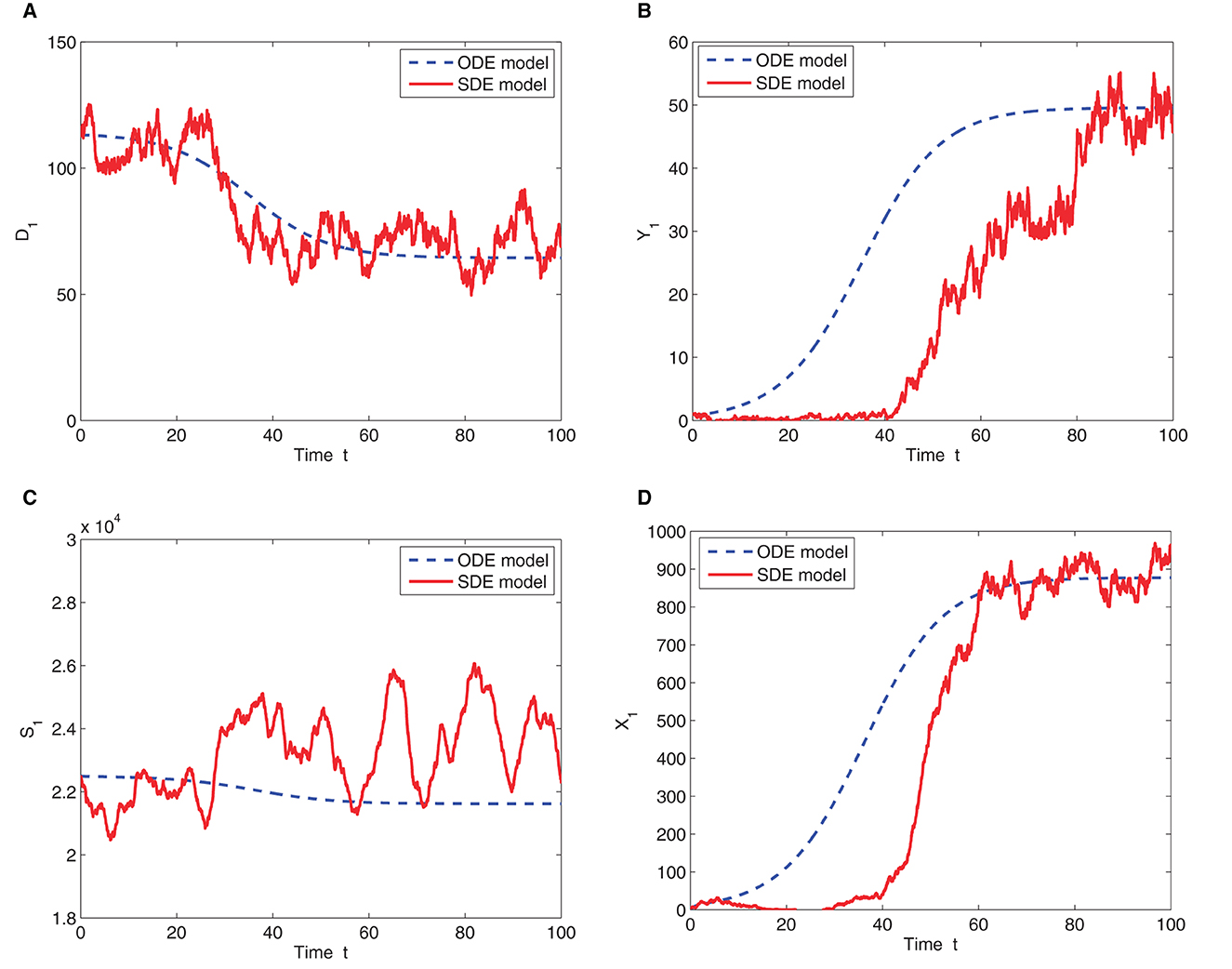
Figure 3. One sample path and ODE solution for the two-patch SDE and ODE models, respectively. The graphs represent the (A) number of susceptible deer in patch 1 (B) number of infected deer in patch 1 (C) number of susceptible ticks in patch 1 and (D) number of infected ticks in patch 1. Time is in months for all the graphs. Initial conditions are D₁(0) = 114, Y₁(0) = 1, S₁(0) = 22, 496, and X₁(0) = 1. Parameter values are given in Table 2 with K = 120 and m = 0. The basic reproduction number ℜ₀ = 1.3571.

TABLE 3

Table 3. The stable endemic equilibrium values for the two-patch ODE model in Figures 3, 4.

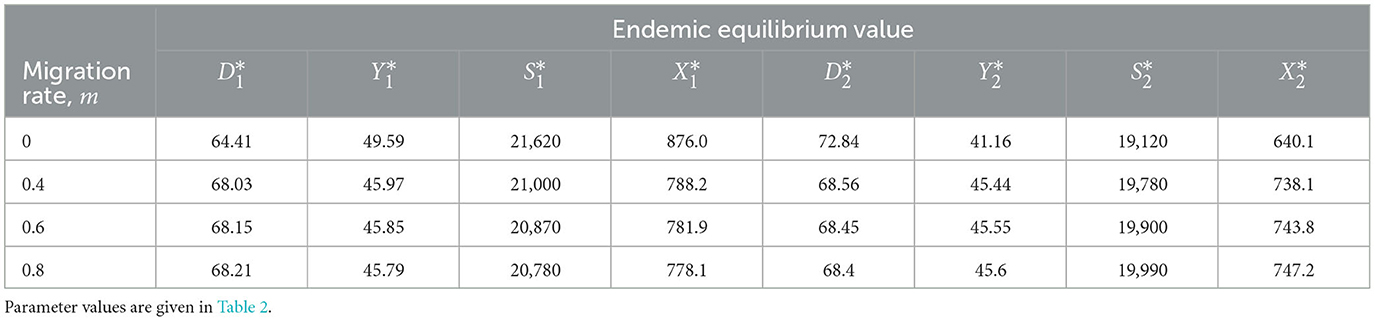
We now consider the case where the patches are connected (m>0) and the migration of the deer and ticks from patch 1 to patch 2 and vice versa is allowed. The ODE and SDE model solutions are graphed in Figure 4 for migration rates of m = 0.6. Figure 4 shows that the SDE model is close to the ODE model and both models predict the same outcome. The number of infected deer and ticks in both patches increases which indicates that the disease invades the susceptible population and converges to a stable endemic equilibrium (see the values for each value of m in Table 3) because ℜ₀>1. Even though the predictions of the ODE and SDE models are similar, there is a possibility that the sample paths of the SDE model will hit zero (disease extinction) in finite time, thereby diverging from the ODE model prediction of disease outbreak.

FIGURE 4

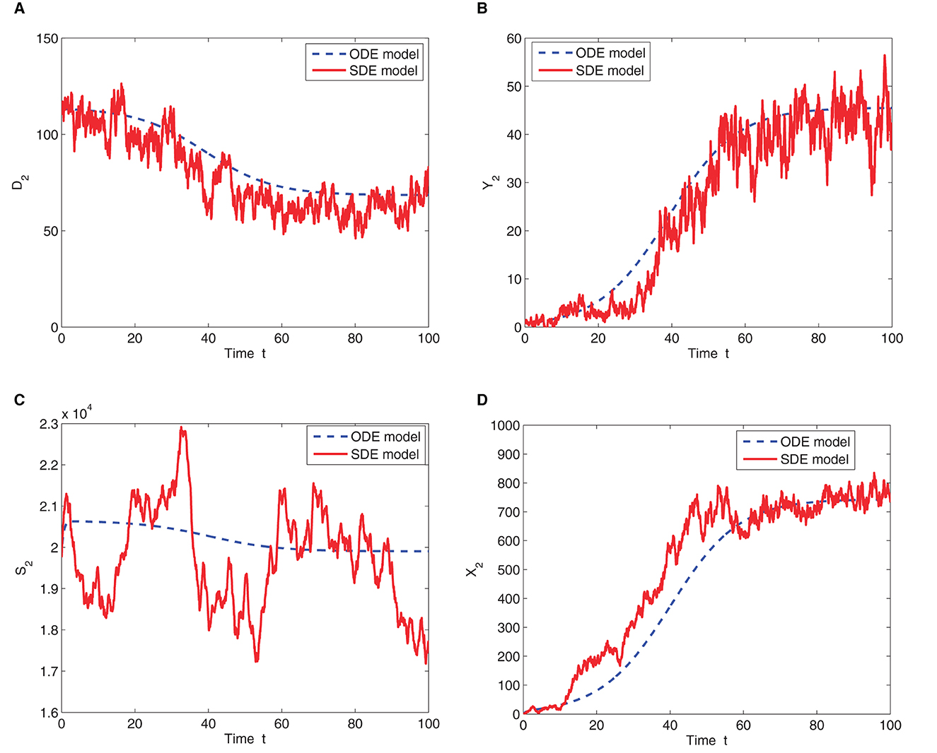
Figure 4. One sample path and ODE solution for the two-patch SDE and ODE models, respectively. The graphs represent the (A) number of susceptible deer in patch 2 (B) number of infected deer in patch 2 (C) number of susceptible ticks in patch 2 and (D) number of infected ticks in patch 2. Time is in months for all the graphs. Initial conditions are D₂(0) = 114, Y₂(0) = 1, S₂(0) = 22, 496, and X₂(0) = 1. Parameter values are given in Table 2 with K = 120, m = 0.6 and ℜ₀ = 1.3154.

It is clear from the disease dynamics of the ODE and SDE models illustrated by the graphs in Figures 3, 4, that migration of susceptible and infected deer (and ticks) from patch 1 to patch 2 and vice versa may enhance disease invasion and subsequently increase the probability of disease outbreak when the disease becomes endemic in both patches for ℜ₀>1.

Figure 5A illustrates the graph of the values of ℜ₀ plotted as a function of the migration rate, m. It is observed that the value of ℜ₀ decreases as m increases but becomes almost constant for values of m≥0.1 since the migration rate from one patch to the other is the same. Although this is the case, ℜ₀ remains greater than 1 and depends on the migration rate of infected deer and ticks. If $\underset{m\to \infty }{lim}{\Re }_0<1$ and the migration rate, m, of infected deer and ticks is sufficiently large, then the disease will not persist in both patches [7, 37]. The probability of disease extinction, P_ext, is also graphed as a function of m in Figure 5B. P_ext is estimated from the proportion of sample paths (out of 10,000) of the two-patch SDE model in which the sum of the infected deer and ticks in both patches, Y₁(t)+Y₂(t)+X₁(t)+X₂(t), equals zero (disease extinction). From the graph in Figure 5B, P_ext is highest when the patches are isolated (m = 0). However, P_ext decreases and becomes almost constant as the values of m increase. Another observation worth noting is that P_ext is lower for m = 1 because when migration is at its peak, disease spread between the patches is enhanced thereby reducing the probability of disease extinction. This is the reason P_ext is highest when m = 0. Figure 5B implies that there is a high probability of achieving a disease-free status or minimizing the disease in both patches when the migration rate is zero (for isolated patches) or very small (for connected patches) unlike when it is large. High rate of migration results in a small probability of extinction which in turn increases the likelihood of disease outbreak. This observation agrees with [9] in that migration can significantly affect the probability of disease persistence in an area.

FIGURE 5

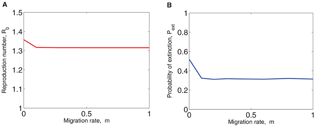
Figure 5. (A) The basic reproduction number, ℜ₀ and (B) the probability of disease extinction, P_ext plotted as functions of the migration rate, m. Initial conditions and parameter values are the same as in Figure 3. The probability of extinction is estimated from 10,000 sample paths of the two-patch SDE model.

The finite-time extinction, T, is one of the important properties of stochastic epidemic models [20]. T is defined as the time it takes until the number of infectious individuals asymptotically approaches zero [9, 20]. Figure 6 shows the graphs of the probability histogram for the two-patch SDE model. The mean time until extinction, T, for graphs in Figures 6A–C is 14.9, 4.1, and 3.9, respectively. T can be very short or very long and depends on, among other factors, the value of the basic reproduction number, ℜ₀ [20]. Thus, the bigger the basic reproduction number, the longer the time until extinction.

FIGURE 6

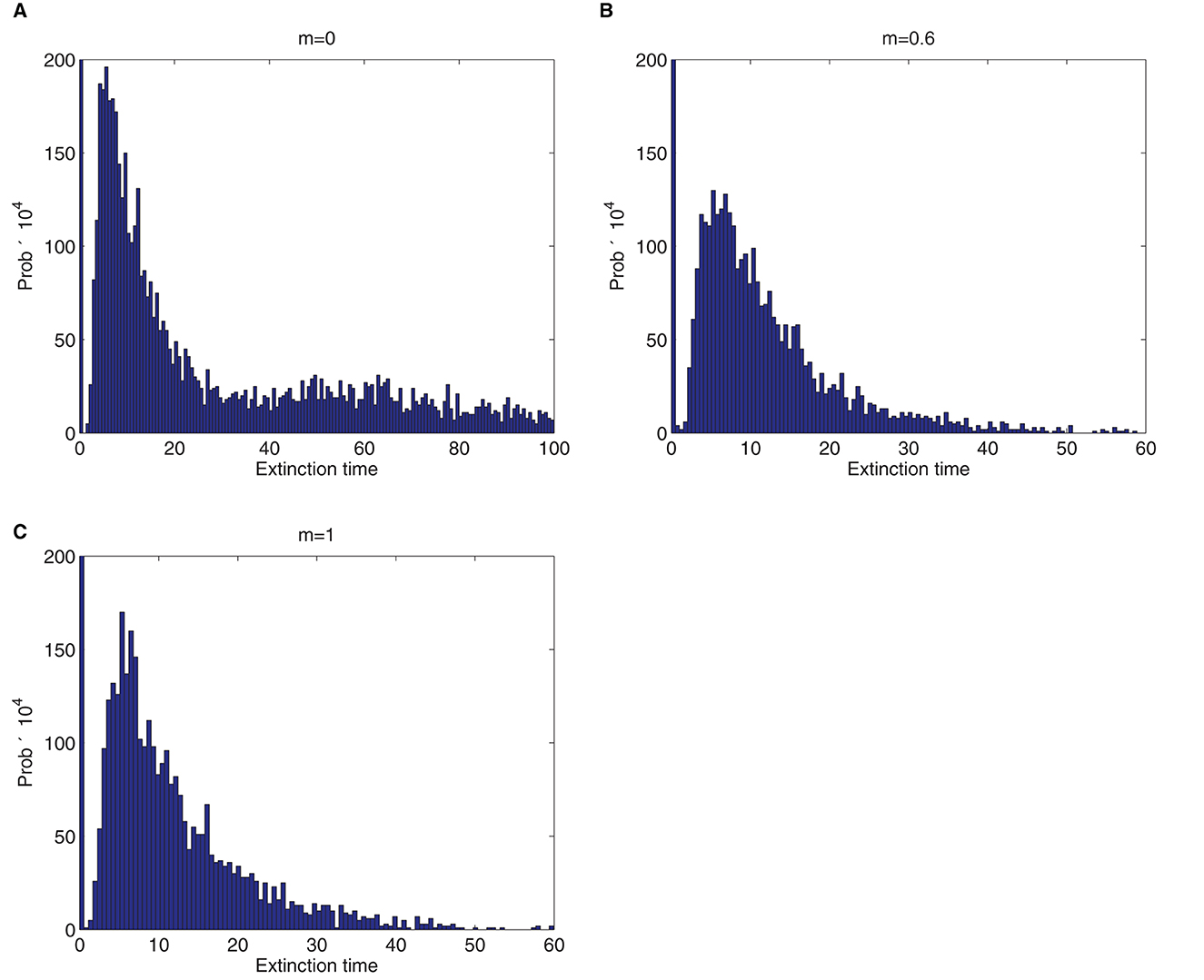
Figure 6. Approximate probability histogram for the time (in months) until disease extinction, T of the two-patch SDE model when there is a single infected deer and tick in both patches. The initial conditions and parameter values are the same as in Figure 3. The value of m is indicated above each graph. The reproduction numbers, ℜ₀ for graphs (A–C) are 1.3571, 1.3154, and 1.3152, respectively. The computations are based on 10,000 sample paths.

5. Conclusion

The spread of pathogens that cause tick-borne diseases can be enhanced by migration of host and ticks from one habitat to another. In this paper, we investigated the impact of migration of the white-tailed deer and lone star ticks on disease dynamics of a tick-borne disease, HME, with respect to spatial spread, extinction and persistence by using a system of Itô stochastic differential equations that was derived from an ODE multipatch model. To achieve this goal, we formulated a general SDE multipatch epidemic model from a multipatch ODE model (see Equation 23) which was later reduced to a two-patch model in numerical simulations.

We showed and proved that the disease-free equilibrium for the ODE multipatch model exists and is unique (see Theorem 1). Also, the general formula for computing the basic reproduction number, ℜ₀, for w patches in the metapopulation was derived using the next generation matrix approach. It was found that ℜ₀ for isolated patches is equal to the largest patch reproduction number (see Theorem 3) and for connected patches, ℜ₀ lies between the minimum and maximum of the patch reproduction numbers (see Theorem 4). When the patch reproduction number ${\Re }_0^j<1$ and ${\Re }_0^j>1$ for all j, the disease dies out and persists in the population, respectively. In addition, if ${\Re }_0^j<1$ in patch j, then the disease dies out in patch j while if ${\Re }_0^j>1$ in patch j, then the disease persists in patch j. When all the patches in the metapopulation are identical, ℜ₀ is equal to ${\Re }_0^j$ and is the same for all patches.

Numerical simulations were performed for two-patch ODE and SDE epidemic models only in order to illustrate the disease dynamics for varying migration rates, m. Our results showed that for ℜ₀>1, the ODE model predicts a stable endemic equilibrium and hence disease persistence (see Figures 3–6) while the SDE model predicts either disease extinction (see Figure 3) or disease persistence (refer to Figures 4–6). This behavior is one of the major differences between deterministic and stochastic epidemic models [3, 20] and is due to demographic stochasticity that is inherent in the system [7, 9, 19]. The predictions made by the two-patch ODE and SDE models with regard to disease extinction and persistence when ℜ₀>1, are the same as the single population models studied by Maliyoni et al. [3]. The probability of disease extinction, P_ext, was numerically computed using 10,000 sample paths. It was observed that the probability of disease extinction is high for isolated patches (no migration) but decreases as migration rate increases (see Figure 5B). In addition, P_ext is lower when m = 1 because when migration rate is highest, the spread of the disease between the patches is fueled and reduces P_ext. Thus, the probability of eliminating or minimizing the disease in both patches is high when there is no migration unlike when it is present. The high migration rate leads to a small probability of extinction thereby increasing the probability of a disease outbreak. This result confirms that migration has a significant impact on the probability of disease persistence as also observed in [9]. The results also showed that ℜ₀ is high when the patches are isolated but slightly decreases when the patches are connected (see Figure 5A), though it remains greater than one and hence endemic. The finite-time extinction, T, was approximated numerically using 10,000 sample paths of the two-patch SDE model. It was found that T is long for large values of ℜ₀ as illustrated in Figure 6.

Our results imply that the probability of disease extinction can be increased if deer and tick movement are controlled (even prohibited) especially when there is an outbreak in one or both patches since movement can introduce a disease in an area that was initially disease-free. Thus, screening of infectives in protected areas (e.g., deer farms, private game parks or reserves, etc.) before they migrate to other areas can be one of the methods for controlling and preventing disease spread. Lahodny and Allen [9] argued that susceptible movement is not significant at the beginning of an epidemic since their population is assumed to be large but after the commencement of a disease outbreak, their movement should be taken into account in controlling further disease spread. Effective control measures for TBDs must also be implemented as quickly as possible whenever there is an outbreak in any of the patches so that the disease does not spread to other patches. We, therefore, agree with Gaff and Schaefer [1] that the areas where control measures are applied could significantly affect the integrity of control efforts. In addition, deliberate efforts aimed at reducing the value of the basic reproduction number, which in turn shortens the time to disease extinction, should be a priority to relevant authorities.

The models formulated in this study can be improved in future studies on TBD, HME. For instance, incorporating environmental stochasticity in the SDE model can provide more insights about HME disease dynamics since deer and ticks are affected by seasonal or environmental variations. Numerical analysis of the models for three or more patches can tell us more about the disease dynamics when individuals move across many patches. In addition, the effectiveness of several control strategies for TBDs can be assessed using the probability of disease extinction and real data (if available). Even though the models in this study focus on a TBD, HME, we believe that with proper model and parameter modifications, they can also apply to diseases that are caused by other tick species and vector-borne diseases with similar behavior to the one described in this paper.

Data availability statement

The original contributions presented in the study are included in the article/Supplementary material, further inquiries can be directed to the corresponding author.

Author contributions

HG provided the biological aspects of ticks and tick-borne diseases (TBDs) which formed the basis of the models in this manuscript and critically checked that the results were making biological sense as far as ticks and TBDs are concerned. MM, FC, and KG developed and analyzed both the ODE and SDE models and interpreted the results. MM carried out numerical simulations of the models which were closely supervised by FC. All authors conceived the idea and problem in this manuscript and refined it until it was in the present form and proofread the manuscript to ensure that it is free of typographical and grammatical errors. All authors contributed to the article and approved the submitted version.

Funding

MM was grateful for the financial support from his employer, the University of Malawi and the University of KwaZulu-Natal (UKZN) throughout his doctoral study duration. KG was thankful to UKZN and the National Research Foundation (NRF) of South Africa for continued research support. FC was supported by the NRF IPRR grant with Grant No: 132253.

Conflict of interest

The authors declare that the research was conducted in the absence of any commercial or financial relationships that could be construed as a potential conflict of interest.

Publisher's note

All claims expressed in this article are solely those of the authors and do not necessarily represent those of their affiliated organizations, or those of the publisher, the editors and the reviewers. Any product that may be evaluated in this article, or claim that may be made by its manufacturer, is not guaranteed or endorsed by the publisher.

Supplementary material

The Supplementary Material for this article can be found online at: https://www.frontiersin.org/articles/10.3389/fams.2023.1122410/full#supplementary-material

References

1. Gaff H, Schaefer E. Metapopulation models in tick-borne disease transmission modelling. In:Michael E, Spear RC, , editors. Modelling Parasite Transmission and Control. New York, NY: Springer (2010). p. 51–65.

PubMed Abstract | Google Scholar

2. Gaff HD, Gross JL. Modeling tick-borne disease: a metapopulation model. Bull Math Biol. (2007) 69:265–88. doi: 10.1007/s11538-006-9125-5

PubMed Abstract | CrossRef Full Text | Google Scholar

3. Maliyoni M, Chirove F, Gaff HD, Govinder KS. A stochastic tick-borne disease model: exploring the probability of pathogen persistence. Bull Math Biol. (2017) 79:1999–2021. doi: 10.1007/s11538-017-0317-y

PubMed Abstract | CrossRef Full Text | Google Scholar

4. Ismail N, Bloch KC, McBride JW. Human ehrlichiosis and anaplasmosis. Clin Lab Med. (2010) 30: 261–92. doi: 10.1016/j.cll.2009.10.004

PubMed Abstract | CrossRef Full Text | Google Scholar

5. Demma LJ, Holman RC, Mcquiston JH, Krebs JW, Swerdlow DL. Epidemiology of human ehrlichiosis and anaplasmosis in the United States, 2001-2002. Am J Trop Med Hyg. (2005) 73:400–9. doi: 10.4269/ajtmh.2005.73.400

PubMed Abstract | CrossRef Full Text | Google Scholar

6. Thomas RJ, Dumler JS, Carlyon JA. Current management of human granulocytic anaplasmosis, human monocytic ehrlichiosis and Ehrlichia ewingii ehrlichiosis. Expert Rev Anti Infect Ther. (2009) 7:709–22. doi: 10.1586/eri.09.44

PubMed Abstract | CrossRef Full Text | Google Scholar

7. McCormack RK, Allen LJS. Multi-patch deterministic and stochastic models for wildlife diseases. J Biol Dyn. (2007) 1:63–85. doi: 10.1080/17513750601032711

PubMed Abstract | CrossRef Full Text | Google Scholar

8. Li S, Hartemink N, Speybroeck N, Vanwambeke SO. Consequences of landscape fragmentation on Lyme disease risk: a cellular automata approach. PLoS ONE. (2012) 7:e39612. doi: 10.1371/journal.pone.0039612

PubMed Abstract | CrossRef Full Text | Google Scholar

9. Lahodny GE Jr., Allen LJS. Probability of a disease outbreak in stochastic multipatch epidemic models. Bull Math Biol. (2013) 75:1157–80. doi: 10.1007/s11538-013-9848-z

PubMed Abstract | CrossRef Full Text | Google Scholar

10. Hygnstrom SE, Groepper SR, VerCauteren KC, Frost CJ, Boner JR, Kinsell TC, Clements GM. Literature review of mule deer and white-tailed deer movements in western and Midwestern landscapes. Great Plains Res. (2008) 18:219–31. Available online at: https://digitalcommons.unl.edu/greatplainsresearch/962/?utm_source=digitalcommons.unl.edu%2Fgreatplainsresearch%2F962&utm_medium=PDF&utm_campaign=PDFCoverPages

Google Scholar

11. Lou Y, Liu L, Gao D. Modeling co-infection of Ixodes tick-borne pathogens. Math Biosci Eng. (2017) 14:1301–16. doi: 10.3934/mbe.2017067

PubMed Abstract | CrossRef Full Text | Google Scholar

12. Guo E, Agusto FB. Baptism of fire: modeling the effects of prescribed fire on Lyme disease. Can J Infect Dis Med Microbiol. (2022) 2022: 5300887. doi: 10.1101/2022.01.01.21268589

PubMed Abstract | CrossRef Full Text | Google Scholar

13. Occhibove F, Kenobi K, Swain M, Risley C. An eco-epidemiological modeling approach to investigate dilution effect in two different tick-borne pathosystems. Ecol Appl. (2022) 32:e2550. doi: 10.1002/eap.2550

PubMed Abstract | CrossRef Full Text | Google Scholar

14. Gaff HD, Nadolny R. Identifying requirements for the invasion of a tick species and tick-borne pathogen through TICKSIM. Math Biosci Eng. (2013) 10:625–35. doi: 10.3934/mbe.2013.10.625

PubMed Abstract | CrossRef Full Text | Google Scholar

15. Glass GE, Schwartz BS, Morgan JM, Johnson DT, Noy PM, Israel E. Environmental risk factors for Lyme disease identified with geographic information systems. Am J Public Health. (1995) 85:944–8.

PubMed Abstract | Google Scholar

16. Arino J, Davis JR, Hartley D, Jordan R, Miller JM, van den Driessche P. A multi-species epidemic model with spatial dynamics. Math Med and Biol. (2005) 22:129–42. doi: 10.1093/imammb/dqi003

PubMed Abstract | CrossRef Full Text | Google Scholar

17. Wang W, Mulone G. Threshold of disease transmission in a patch environment. J Math Anal Appl. (2003) 85:321–35. doi: 10.1016/S0022-247X(03)00428-1

CrossRef Full Text | Google Scholar

18. Allen LJS. An Introduction to Stochastic Processes with Applications to Biology. 2nd ed. Boca Raton, FL: Chapman and Hall/CRC Press (2010).

Google Scholar

19. Kirupaharan N, Allen LJS. Coexistence of multiple pathogen strains in stochastic epidemic models with density-dependent mortality. Bull Math Biol. (2004) 66:841–64. doi: 10.1016/j.bulm.2003.11.007

PubMed Abstract | CrossRef Full Text | Google Scholar

20. Allen LJS. An introduction to stochastic epidemic models. In:Brauer F, van den Driessche P, Wu J, , editors. Mathematical Epidemiology. Berlin: Springer (2008). p. 77–128.

Google Scholar

21. Allen LJS. A primer on stochastic epidemic models: formulation, numerical simulation and analysis. Infect Dis Model. (2017) 2:128–42. doi: 10.1016/j.idm.2017.03.001

PubMed Abstract | CrossRef Full Text | Google Scholar

22. Allen EJ, Victory HD Jr. Modelling and simulation of a schistosomiasis infection with biological control. Acta Trop. (2003) 87:251–67. doi: 10.1016/S0001-706X(03)00065-2

PubMed Abstract | CrossRef Full Text | Google Scholar

23. Allen EJ, Allen LJS, Schurz H. A comparison of persistence-time estimation for discrete and continuous stochastic population models that include demographic and environmental variability. Math Biosci. (2005) 196:14–38. doi: 10.1016/j.mbs.2005.03.010

PubMed Abstract | CrossRef Full Text | Google Scholar

24. Allen EJ. Stochastic differential equations and persistence time for two interacting populations. Dyn Cont Dis Impul Syst. (1999) 5:271–81.

Google Scholar

25. McCormack RK. Multi-host and multi-patch mathematical epidemic models for disease emergence with applications to hantavirus in wild rodents. Ph.D. dissertation. Texas Tech University, Lubbock, TX, United States (2006).

Google Scholar

26. Gao D, Ruan S. A multi-patch malaria model with logistic growth populations. SIAM J Appl Math. (2012) 72:819–41. doi: 10.1137/110850761

PubMed Abstract | CrossRef Full Text | Google Scholar

27. Berman A, Plemmons RJ. Non-Negative Matrices in Mathematical Sciences. New York, NY: Academic Press (1979).

Google Scholar

28. Qiu Z, Kong Q, Li X, Martcheva M. The vector-host epidemic model with multiple strains in a patchy environment. J Math Anal Appl. (2013) 405:12–36. doi: 10.1016/j.jmaa.2013.03.042

CrossRef Full Text | Google Scholar

29. van den Driessche P, Watmough J. Reproduction numbers and sub-threshold endemic equilibria for compartmental models of disease transmission. Math Biosci. (2002) 180:29–48. doi: 10.1016/S0025-5564(02)00108-6

PubMed Abstract | CrossRef Full Text | Google Scholar

30. van den Driessche P. Spatial structure: patch models. In:Brauer F, van den Driessche P, Wu J, , editors. Mathematical Epidemiology. Berlin; Heidelberg: Springer (2008). p. 179–89.

Google Scholar

31. Allen EJ. Modelling with Itô Stochastic Differential Equations. Dordrecht: Springer (2007).

Google Scholar

32. Allen LJS, Lahodny GE Jr. Extinction thresholds in deterministic and stochastic epidemic models. J Biol Dyn. (2012) 6:590–611. doi: 10.1080/17513758.2012.665502

PubMed Abstract | CrossRef Full Text | Google Scholar

33. Allen EJ, Allen LJS, Arciniega A, Greenwood P. Construction of equivalent stochastic differential equation models. Stoch Anal Appl. (2008) 26:274–97. doi: 10.1080/07362990701857129

CrossRef Full Text | Google Scholar

34. Øksendal B. Stochastic Differential Equations: An Introduction with Applications. 5th ed. Berlin: Springer (2000).

PubMed Abstract | Google Scholar

35. Øksendal B. Stochastic Differential Equations. 2nd ed. New York, NY: Springer-Verlag (1989).

Google Scholar

36. Kloeden PE, Platen E. Numerical Solution of Stochastic Differential Equations. New York, NY: Springer (1992).

PubMed Abstract | Google Scholar

37. Salmani M, van den Driessche P. A model for disease transmission in a patchy environment. Discrete Contin Dyn Syst Ser B. (2006) 6:185–202. doi: 10.3934/dcdsb.2006.6.185

CrossRef Full Text | Google Scholar