An implementation of Hurdle models for spatial count data. Study case: civil war as a risk factor for the development of childhood leukemia in Colombia

1. Introduction

The effects of violent environments that generate recurrent adverse childhood events (ACEs) have been identified as risk factors for some chronic diseases in adulthood. The term “Toxic Stress” is defined “as the exposure to extreme, frequent and persistent adverse events without the present of a supportive caretaker” [1]. Toxic stress is differentiated from other types of stress in two notable ways: First, its sources are severe, prolonged, unpredictable, and/or unrelenting; and second, it represents a hijacking of the normal stress response mechanisms mediated by the brain [1]. This association has been seen even if the exposure occurs during gestation, where the external maternal environment could cause changes at the genetic and transcriptional level in the growing fetus [2]. Violence and chronic stress during pregnancy were associated with congenital malformations, intellectual disability, growth retardation, and other complications for both the mother and the child [3]. The biological explanation of the association between exposure to toxic stress and diseases such as cancer is described in epigenetics by the “two hits” model, see [4–6]. The first “hit” occurs when the transcriptional control that regulates gene activity is altered. Translocations and the production of fusion genes arise as a response to chronic stress in the external maternal environment: violence, malnutrition, and poverty, among others, see [7, 8]. The second exposure to chronic and toxic stress during the child's life leads to the second “hit” with the proliferation of malignant cells, given that the neuroendocrine system is permanently activated. see details in [8–10].

Early and persistent exposure to chronic stress generates lasting damage to the nervous, endocrine, and immune systems through DNA alteration [11, 12]. Neurobiological effects of violence against children produce a decrease in the volume of the hippocampus and prefrontal cortex [12] and elevated levels of C-reactive protein, IL-6, TNF-α, and IL-1β, see [13–15]. Concerning cancer, the chronic activation of the neuroendocrine system alters the profile of counter-regulatory hormones that modulate the activity of multiple components of the tumor microenvironment, such as DNA repair, the expression of oncogenes by viruses and oncogenic cells, and the production of cell growth factors [5]. Once the tumor starts its development, variables that regulate the activity of proteases, angiogenic factors, chemokines, and adhesion molecules, allow for invasion, metastasis, and other aspects of tumor progression [10, 16].

Colombia is a country struck by a civil war since the 1950s [17]. The main actors are insurgent groups such as guerrillas, paramilitary groups, drug traffickers, common crime groups, and the Colombian military forces [18]. During 2002–2013, more than 30% of the Colombian population lived in extreme poverty. Children with and without neoplastic diseases living in conflict-affected areas and/or in extreme poverty do not have timely health service [19]. For example, they face outbreaks of vaccine-preventable diseases. Civil war and poverty also reduce school attendance, increase unemployment rates, prevent food production in rural areas, and generate slowdowns in the economy and the erosion of human capital [20]. Civilians have had to be witnesses and victims of all of these actions that lead to chronic stress environments [1, 21]. Children have lost the right to health, and they live in environments of fear, hopelessness, and chronic uncertainty [20]. They have suffered the effects of antipersonnel mines, forced displacement with or without their family, kidnappings, murders and massacres of their relatives or neighbors, being children of combatants, demobilization of their parents, abuse and neglect, attacks, and armed clashes, spraying of illicit crops, among others. Thus, children suffer severe damage that changes their lives and those of their subsequent generations. Research on this topic is scarce because these effects on children are underestimated and considered low-priority problems [22].

In addition, statistical models for count data, such as the number of cases of some illness per area, faced issues like overdispersion, zero excess, and spatial association. These are usually fitted, keeping all data in the same model and using the independence assumption. Hence, data with these features needs a specific methodology that allows us to consider all the richness of the available information.

So, the aims of this study are two: First, to propose and implement a methodology to describe and model data with features as those we encountered here: high variance, excess of zeros, and spatial association, and Second, to apply the proposal to explore, test, and quantify the association among the civil war and poverty in Colombia, and childhood leukemia incidence and mortality. It is well-known that a country's poverty has specific spatial patterns, see [23, 24]. However, to our knowledge, no studies are exploring or modeling the spatial correlation of the Colombian armed conflict and its impact on the development of Leukemia. One of the main barriers is acquiring a complete and good-quality Datasets.

We propose a novel approach for the estimation of spatial generalized linear models by combining Poisson-Hurdle models, the Moran coefficient, and Moran Eigenvectors Spatial Filtering. Based on this procedure, it is possible to manage data with spatial correlation and more variability in response variables than is expected under usual models for count data. Hurdle models are statistical models that separate the random variable values into two parts: the first part models the probability of the 0 value, and the second part models the probability of the non-zero values. The spatial information is involved in several ways. The residuals of the estimated model under independence are used to validate this assumption and when the independence assumption is not fulfilled, the best spatial weights matrix to find the Moran coefficient is determined. Finally, we use lagged explanatory variables and Moran Eigenvectors as predictors, to find a valid model with good fitting. This proposal aims to investigate how armed conflict affects the incidence and mortality rate of LAP in children. The Index of Incidence of Armed Conflict (IICA), developed recently as a result of the Colombian peace process, by the National Planning Department, is the first opportunity to quantify the impact of the civil war on the population across the country. The paper follows with the methodological setup in Section 2, and description of real dataset and results in Section 3. The paper ends with some concluding remarks and future work in Section 4.

2. Materials and methods

Hurdle models present a methodology to treat excess zeros through mixture and truncated distributions [25]. We here adapt the Poisson Hurdle models, due to features of our study case, but analogous Hurdle Models can be adapted, according to response variable distribution, see [25] and Figure 6. Generalized linear models are built under the independence assumption. By default, in the first stage, the fitting process does not consider any type of correlation. Hence, it is necessary to check model assumptions using the residual vector. Correlation tests make sense and are useful when there is some knowledge about the origin of the existing correlation. Based on this knowledge and test results, the correlation structure is estimated and involved in the model approach and fitting, in the next stage.

2.1. Poisson-Hurdle models

The response variable is based on count data with an excess of zero counts. Although there are several alternatives, we choose Hurdle models because one of its advantages is that by design the number of zeros predicted is the same as the number of zeros observed. Given that the excess zeros can be generated by a separate process from the count values, the observations are separated into two subsets: the first one with zeros and the second one with positive counts, so, it is obtained the following binomial distribution:

$\begin{array}{ll}\{\begin{array}{l}P\left(Z_i=0\right)=p,\hfill \\ P(Z_i=k)=(1-p)\frac{{\mu }_i^k\exp (-{\mu }_i)}{(1-\exp (-{\mu }_i))k!}\hfill \end{array}& (1)\end{array}$

Where k ∈ ℕ − {0}, p is the probability of a count of zero and Z_i is the count response variable in the municipality i. Thus, p_i can be modeled with a logistic regression and positive counts can be modeled with a truncated Poisson model, that is,

$\begin{array}{ll}ln\left(\frac{p_i}{1-p_i}\right)=x_i^{\prime }\beta \text{\hspace{1em} and\hspace{1em} }ln({\mu }_i)=x_i^{\prime }\alpha & (2)\end{array}$

Where x_i is the vector containing predictor variables, and β and α are vectors of regression coefficients, respectively. In addition, if positive counts are observed from exposure n_i, the link function for positive counts is

$\begin{array}{ll}E(Z_i>0)={\mu }_i=n_{i}exp(x_i^{\prime }\alpha )& (3)\end{array}$

n_i is the offset term, and

$\begin{array}{ll}ln{\mu }_i=ln{n}_i+x_i^{\prime }\alpha & (4)\end{array}$

2.2. Lattice data

Data associated with spatial subregions which are elements of a partition of some region of interest are called lattice data or areal data. Thus, areal data have discrete spatial variation. It is very common that for economic, epidemiology, or public health data, this partition corresponds to the official administrative political division. However, the partition can also be determined according to each problem. For example, quadrats in ecological studies. Usually, in this context, information is available for all subregions: The gross domestic product by department or the number of live births by municipality. Therefore, in most cases, the purpose is not the prediction, but the estimation of regression models involving and quantifying spatial dependence, to determine the significance of covariates or the detection of spatial patterns. Z(s) is the response spatial random variable. D_s is the region of interest, and it is partitioned into N subregions

$A=\left\{A_1,A_2,...,A_N\right\}$

To identify these subregions, it is established a representative coordinate, s_i for each polygon A_i, i = 1, ..., N. These coordinates are known as centroids and can be determined by geometric methods or according to criteria related to each particular study. S defined as

$\text{S}=\left\{{\text{s}}_1,{\text{s}}_2,...,{\text{s}}_{{}_N}\right\}s\in D_{\mathit{s}}$

is the set of centroids. Then Z(A_i) with i = 1, ..., N represents the spatial process in the region A_i with i = 1, ..., N. Its observation is denoted z(s_i).

2.3. Spatial weight matrix

Our hypothesis is the existence of spatial correlation given the similar conditions among areal units. In this context, each observation corresponds to a specific areal unit. The set of these areal units is a partition of the region of interest. Spatial correlation measures the relationship among variables in a specific areal unit and variables in its spatial neighborhood. The estimation of spatial correlation is based on spatial contiguity relations, represented graphically as a network, see [26] for a good exposition.

The quantification of these relations according to some criterion, such as spatial proximity or relevant features, is summarized in a square matrix W, of dimension N × N, called spatial weight matrix. W is non-stochastic, with real, non-negative, and finite entries, representing spatial interdependence between areal units [27]. W defines the magnitude of spatial interactions inside a region:

$W=(w_{ij})=\left(\begin{array}{ccccc}0& w_{12}& w_{13}& \dots & w_{1N}\\ w_{{}_{21}}& 0& w_{23}& \dots & w_{2N}\\ w_{31}& w_{32}& 0& \dots & w_{3N}\\ ⋮& ⋮& ⋮& \ddots & ⋮\\ w_{N1}& w_{N2}& w_{N3}& \dots & 0\end{array}\right)$

i, j = 1, ..., N. Non-zero entries indicate related spatial areal units. W considers the spatial multidirectional relations. The spatial weights matrix W acts as a spatial lag operator. By performing its product with the observations vector, a lag vector resulting from a linear combination is obtained. Each observation is multiplied by its respective spatial weight with the rest of the spatial observations: WZ.

In this matrix, all possible pairs of observations are included, and each other influence is determined. The row i is the vector of spatial weights between Z(s_j), j = 1, ..., N and Z(s_i). This matrix is supposed to be known, and it is not part of the elements to be estimated within the model. W must be previously defined since it enters the estimation processes as a constant. The correct specification of the way in which individuals interact is crucial.

There are multiple criteria to generate its values. The most used criteria are those that generate binary weights matrices, assigning the value of one to the contiguous units and zero to the others. Criticisms of the binary relations are the symmetry that is imposed on spatial relationships and the use of physical adjacency as the only criterion. Other criteria are based on associated graph measurements involving distances between the centroids of the regions considered, shared borders, and even covariates can be considered. The standardized weights matrices are built from the binary relations, and each w_ij is weighted by the sum of its row; this transformation incorporates asymmetry in W. See [28] for more details. The asymmetry can generate theoretical complications, and often it is replaced by the product with its transpose in later stages.

Below, we describe some criteria to build the matrix W. Some of them take physical contiguity into account; others are based on associated graph measurements, or involve computing distances between the centroids of the regions considered:

• Rock criterion: Areal units are neighbors if share a common edge.

• Queen criterion: Areal units are neighbors if share a common edge or a common vertex.

• Gabriel graph: Areal units are neighbors if

$\begin{array}{l}d({\mathit{s}}_i,{\text{s}}_j)\le min\left\{\sqrt{{(d({\text{s}}_i,{\text{s}}_k))}^2+{(d({\text{s}}_j,{\text{s}}_k))}^2}|\forall {\text{s}}_k\in \text{S}\right\}\end{array}$

• k-Nearest neighbors:. In this case, relations are established using non-symmetrical distances and standardized spatial weight matrices. The neighborhood criterion chooses, for each s_i, the k-nearest units. So, the rest of the data

$k+1,k+2,...,k+m$

are considered non-neighbors of s_i.

• Relative neighbors: According to this criterion, areal units are neighbors if

$d({\mathit{s}}_i,{\mathit{s}}_j)\le min{(maxd({\mathit{s}}_i,{\mathit{s}}_j),d(y,{\mathit{s}}_k))}^{1/2}$

• Using distance for weighting,

$w_{ij}=1-d_{ij}/max(d_{ij})$

Where d_ij is the distance between the units centroids. Note that similarity is inversely proportional to distance.

For illustrative purposes, we show maps and neighbors with its graphs, to observe the behavior of a criterion with different orders of neighbors, in two cases: The 1,124 Colombian Municipalities and the 85 departments of France [29], see Figure 1. In both cases, the queen criterion is used. However, for the French departments, first, second, and third-order neighbors are included, while for Colombia, it included only the first neighbor. The spatial weights matrix W is built based on the graph generated according to each of the criteria. Thus, it is important to establish some rules to select a criterion, see Section 2.4 and [30].

FIGURE 1

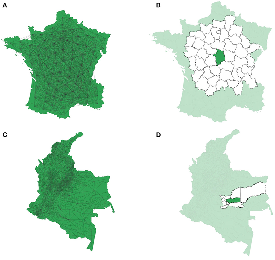
Figure 1. (A) Complete graph for French departments [29], using the queen criterion and including first, second, and third-order neighbors. (B) White areas are first, second, and third-order neighbors in every direction for the highlighted department. (C) Complete graph for Colombian municipalities, using the queen criterion and first-order neighbors. (D) White areas are the first neighbors in every direction for the highlighted municipality.

2.4. Moran coefficient (MC)

The areal data are observations associated with spatial subregions that are elements of a partition of the complete region of interest. It is very common that for economic, epidemiology, or public health data, this partition corresponds to the official administrative political division. However, the partition can also be determined according to each problem. For example, quadrats in ecological studies. Usually, in this context, information is available for all subregions. For example, the gross domestic product by department or the number of live births by municipality. Therefore, in most cases, the purpose is not the prediction, but the estimation of regression models involving and quantifying spatial dependence, to determine the significance of variables involved or to detect spatial patterns.

There are several measures in areal data, to check if there is significant spatial autocorrelation and its sign. In addition, contrasts to detect spatial correlation are of two types, global and local. The former calculates an autocorrelation coefficient for the entire region of interest, while the latter calculates these coefficients in subregions, see Figure 1. Given related theoretical advances truly useful in spatial regression models, we use here the Moran coefficient. This coefficient measures the spatial correlation between each region and its neighbors, extending the idea of the Pearson correlation coefficient for the spatial case. That is, the product moment term is multiplied by its corresponding spatial weight w_ij. When the mean of Z(s) is constant, the Moran coefficient MC is given by:

$\begin{array}{ll}MC=\frac{N}{{\displaystyle \sum _{i=1}^N}{\displaystyle \sum _{j=1}^N}{w}_{ij}}\frac{{\displaystyle \sum _{i=1}^N}{\displaystyle \sum _{j=1}^N}{w}_{ij}(z(s_i)-\bar{z})(z(s_j)-\bar{z})}{{\displaystyle \sum _{i=1}^N}{(z(s_i)-\bar{z})}^2}& (5)\end{array}$

where z(s_i) is the value of Z in the region i, $\bar{z}$ is its mean, w_ij are the weights from the W matrix, i = 1, ..., N. If we denote with $\mathcal{Z}$ the centered vector, MC can be written in matrix form as follows

$MC=\frac{N}{S_0}\frac{{\mathcal{Z}}^{\prime }W\mathcal{Z}}{{\mathcal{Z}}^{\prime }\mathcal{Z}}\text{where\hspace{1em}}{S}_0={\displaystyle \sum _i}{\displaystyle \sum _j}{w}_{ij}$

In the context of spatial regression models, this index is used as a criterion to verify spatial autocorrelation between residuals vector e [31]. So, the MC for the residuals of a regression model is written as

$MC=\frac{N}{S_0}\frac{e^{\prime }We}{e^{\prime }e}\text{where\hspace{1em}}{S}_0={\displaystyle \sum _i}{\displaystyle \sum _j}{w}_{ij}$

The MC has been extended to the bivariate case through Lee's statistics index, L, see [32, 33]. This coefficient measures the spatial cross-correlation between two variables in two different places and also can be global and local. Assuming constant means, the Lee coefficient is given by:

$\begin{array}{c}L=\\ \frac{N}{{\displaystyle \sum _{i=1}^N}{\left({\displaystyle \sum _{j=1}^N}{w}_{ij}\right)}^2}\frac{{\displaystyle \sum _{i=1}^N}\left({\displaystyle \sum _{j=1}^N}{w}_{ij}(z_1(s_j)-{\bar{z}}_1)\right)\left({\displaystyle \sum _{j=1}^N}{w}_{ij}(z_2(s_j)-{\bar{z}}_2)\right)}{{\displaystyle \sum _{i=1}^N}{(z_1(s_i)-{\bar{z}}_1)}^2{\displaystyle \sum _{i=1}^N}{(z_2(s_i)-{\bar{z}}_2)}^2}& (6)\end{array}$

where z₁(s_i) and z₂(s_i) are the values (realizations) of Z₁ and Z₂ in the region i, i = 1, ..., N, ${\bar{z}}_1$ ${\bar{z}}_2$ are the respective means, and w_ij are the elements of the W matrix.

Two L bivariate analyses, between IICA and the two predictors LR and UBN, are shown in Figure 2. The significant cross-correlation is detected through L coefficient and allows identifying the spatial clusters where the two variables show strong association.

FIGURE 2

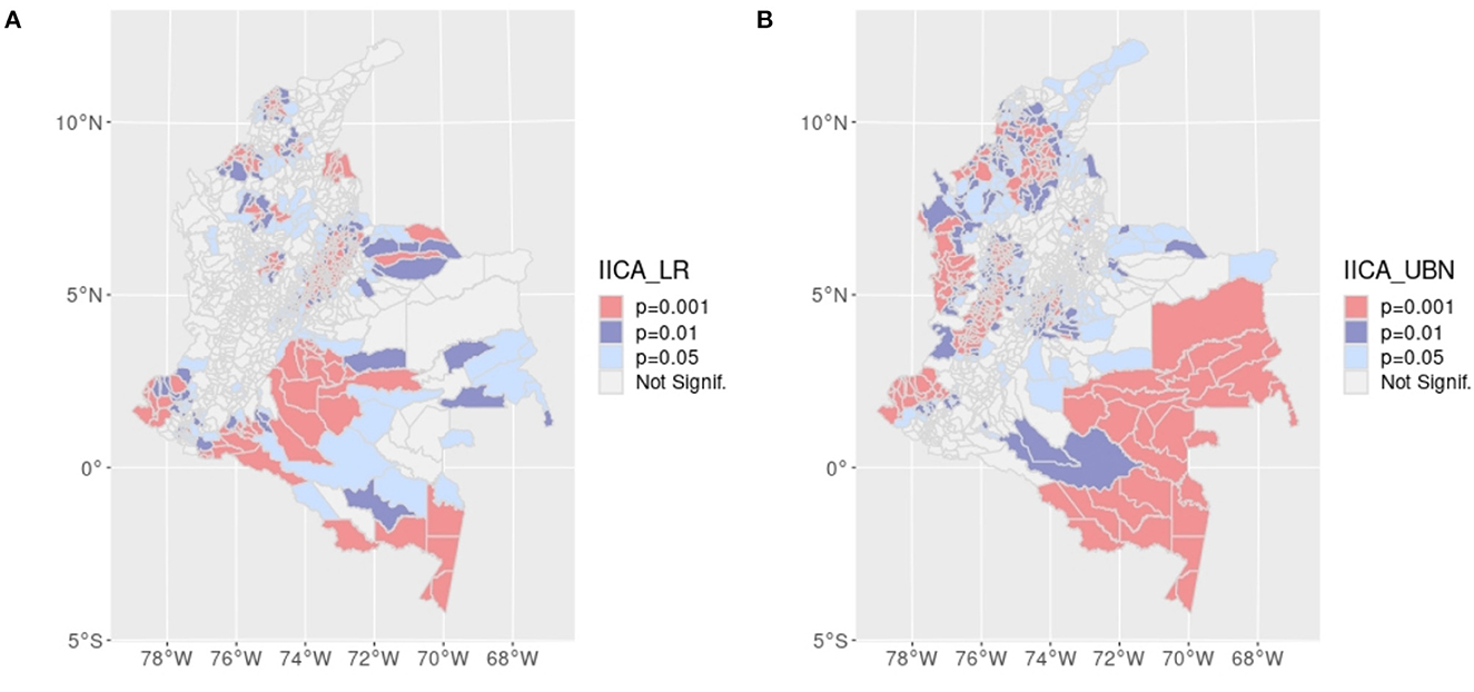
Figure 2. Significance of Bivariate Local Moran Index for spatial association between: (A) IICA with LR. (B) IICA with UBN.

2.5. Inference for the Moran coefficient

Given that the distribution of statistical tests is usually unknown and that a large number of combinations sometimes makes them impossible to find the exact distribution, randomization and Monte Carlo tests are typically used in the inferential process. The associated null hypothesis is the absence of spatial autocorrelation. According to Anselin [27], a positive and significant value of MC indicates a concentration of similar data in neighboring regions: High values of the variable are surrounded by high values, and low values are surrounded by low values. Negative values that lead to rejecting the null hypothesis indicate that high values of the variable are surrounded by low values and low values are surrounded by high values, thus in neighboring units different values are presented.

Let MC₁ be the observed value and let

$M{C}_i:i=2,\cdots ,k$

the k − 1 realizations by random sampling under spatial independence. Then MC₁ is combined with the MC_i and these values are sorted to get the following list

$M{C}_{(1)}M{C}_{(2)}\cdots M{C}_{(k)}$

Tests with MC_i near zero indicate an absence of spatial autocorrelation, while large values of MC_i positive or negative indicate autocorrelation of the same sign. The hypothesis is rejected when

$M{C}_1\le M{C}_{(r)}M{C}_1\ge M{C}_{(k-r)}$

where MC_(r) denotes the r − th smallest value. This is a two-tailed test with a significance level α, which is defined as

$\alpha =\frac{2r}{k}$

Depending on the required α, the number of simulations needed is chosen.

When the sample size is large enough, the standardized Moran coefficient MC, follows an asymptotic normal distribution [27]. That is,

$z_{MC}=\frac{MC-E(MC)}{\sqrt{Var(MC)}}~N(0,1)$

with

$E(MC)=-\frac{1}{N-1}$

and

$\begin{array}{c}E(M{C}^2)=\\ \frac{N\left[(N^2-3N+3)S_1-N{S}_2+3S_0^2\right]-b_2\left[(N^2-N)S_1-2N{S}_2+6S_0^2\right]}{(N-1)(N-2)(N-3)S_0^2}\end{array}$

where

$b_2=\frac{m_4}{m_2^2},m_2=\frac{{\displaystyle \sum _{i=1}^N}{(z(s_i)-\bar{z})}^2}{N},m_4=\frac{{\displaystyle \sum _{i=1}^N}{(z(s_i)-\bar{z})}^4}{N}$

$\begin{array}{c}{S}_1=\frac{1}{2}{\displaystyle \sum _{i=1}^N}{\displaystyle \sum _{j=1}^N}{(w_{ij}+w_{ji})}^2,S_2={\displaystyle \sum _{i=1}^N}{(w_{i·}+w_{{}_{·i}})}^2,\\ w_{i·}={\displaystyle \sum _{j=1}^N}{w}_{ij},w_{·i}={\displaystyle \sum _{j=1}^N}{w}_{ji}\end{array}$

Now, we show the results of the Moran coefficient analysis for IICA, using a spatial weight matrix W built according to queen criteria and first-order neighbors, see Figure 3. The dispersion plot shows IICA vs. WIICA, that is, the observed variable vs. its spatial lag. This variable presents a positive and significant spatial autocorrelation. Note that z − value for the asymptotic normality test is 33.322 having a p ≈ 0. Monte Carlo test with 999 permutations gives a pseudo p = 0.001. So, the spatial autocorrelation is significant at the 95% confidence level.

FIGURE 3

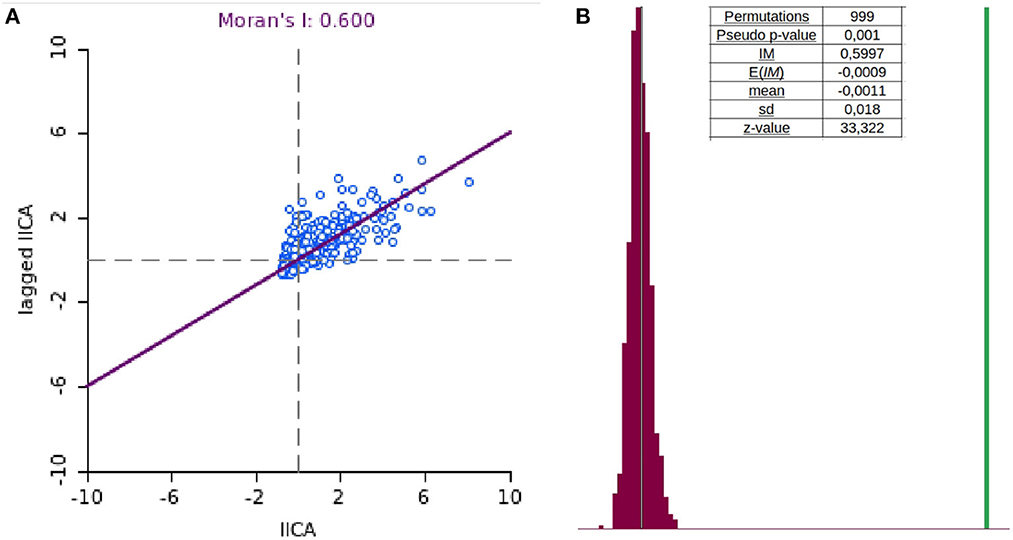
Figure 3. (A) Lagged plot for the Colombian index of armed conflict (IICA), the main variable of this study. For illustrative purposes, the queen criterion is used with one neighbor. Note that the points are located in the first quadrant with a positive slope. MC = 0.6 see Equation 5. The spatial autocorrelation is positive, that is, similar values of IICA are clustered together on the Colombian map. (B) Inference for the Moran coefficient. Both, the Monte Carlo test with 999 permutations and asymptotic normality, indicate significant spatial autocorrelation.

Figure 4 illustrates the local spatial autocorrelation (LISA) analysis using the Moran coefficient, for suicides in France in 1830 [29]. Spatial clusters have been detected. For Colombian data, these analyses are shown in Figure 5.

FIGURE 4

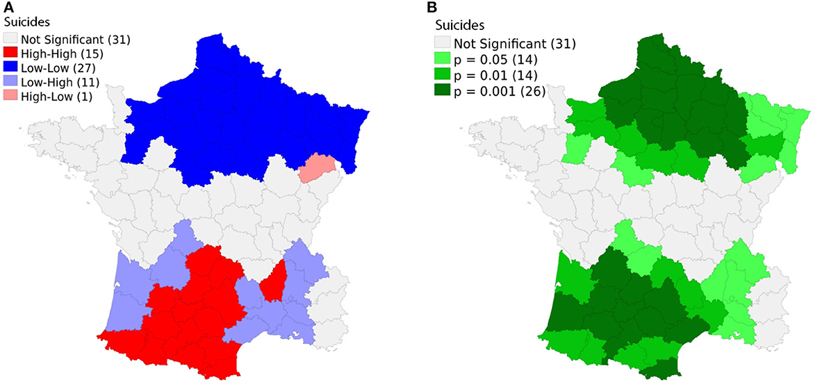
Figure 4. (A) Spatial cluster of suicides in France in 1830 [29]. There are 15 departments with high suicide rates surrounded by similar high values, and 27 departments with low suicide rates surrounded by similar low values. Only one with a high value is near a cluster of low values and 11 low values are near high values. (B) Significance of the local spatial analysis. The white areas do not show significant spatial association. The rest of the cases show significance at 90, 95, or 99% confidence level.

FIGURE 5

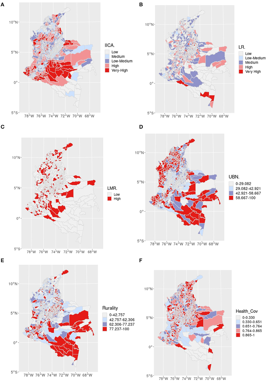
Figure 5. Spatial distribution of variables considered. (A) Colombian index of armed conflict (IICA). (B) Leukemia rate (LR). (C) Leukemia mortality rate (LMR). (D) Unmet basic needs (UBN). (E) Percentage of people living in rural areas (Rurality). (F) Percentage of health coverage (Health Cov).

The Moran index can be strengthened through its articulation with complex networks. It improves the detection of some patterns and behaviors of spatial events. Among complex network metrics, those related to the flow of information stand out. The performance of the models can be improved by quantifying the propagation force of the event by linking spatial dimensions with other information, such as covariates that are present in said places with higher values of the Moran index. On the other hand, with these same results and metrics such as modularity and the clustering coefficient, it is possible to understand the endogenous characteristics that favored the configuration of spatial buffers, or the presence of some spatial point patterns. These elements are very useful for the management of computational complexity [34]. The metrics (modularity, centrality, assortativity, and cluster coefficient) of the networks are expressed in synthetic indicators. They reflect properties of the information system, that facilitate the construction of mining algorithms for the detection of patterns in large volumes of information. On the other hand, these metrics can even be calculated from heuristic approaches and statistical computing (for example, Bootstrap) to boost the speed in obtaining the results without affecting their quality [26, 35].

2.6. Moran eigenvector spatial filtering method

This spatial filtering method pursues to remove the effects of spatial autocorrelation and spatial heterogeneity of model residuals, along with modeling the multiscale nature of the response variable. These goals are accomplished through building and incorporating into the model, new spatial predictor variables based on the residuals of the initial model and on the spatial weights matrix. The estimation procedure is very efficient because it only involves standard generalized linear regression computations. This is an advantage over methods that require the Markov chain Monte Carlo algorithm, have limitations to treating with positive spatial correlation, or involve optimization of intractable expressions [30].

Moran's global autocorrelation criterion MC(.) can be written as follows,

$\begin{array}{l}MC=\frac{N}{1^{\prime }W1}\frac{e^{\prime }\Omega e}{e^{\prime }(I-11^{\prime }/N)e}\text{with}\\ \Omega =(I-11^{\prime }/N)W(I-11^{\prime }/N)& (7)\end{array}$

where I is the N × N identity matrix, 1 denotes the N × 1 vector of ones. W is the N × N spatial weights matrix. The spatial filtering method consists of the spectral decomposition of Ω, using a spatial weights matrix W. MC for an eigenvector obtained h_j, j = 1, ..., N is given by

$\begin{array}{ll}(N/1^{\prime }W1){\lambda }_j& (8)\end{array}$

where λ_j is the j − th eigenvalue. So, the maximum and minimum values of MC are associated with λ_max and λ_min, respectively. Note that MC is not bounded between −1 and 1. Each element of the N×1-eigenvector corresponds to each of the N areal units. Therefore, it has a specific geographic distribution, and it can be included as a covariate in the regression model. Thus, the set of h_i, i = 1, ..., N are known as Maps of Moran Eigenvectors (MEM) [30]. To account for spatial autocorrelation, we use this method, and the set of predictor variables is enlarged with the selected k Moran eigenvectors, H = (h₁, ..., h_k), obtained from spectral decomposition of Ω. So, X is replaced on the count model part, see Section 2.1 by

$(\mathbb{X},H)$

In addition, note that these eigenvectors are mutually uncorrelated and mutually orthogonal. The connectivity matrix W is selected among several neighborhood schemes based on physical contiguity: graphs and distances, using the criterion of minimization of the residual spatial autocorrelation [36], in the final model.

The steps that we should follow to put into practice our methodological proposal are the following:

1. To fit the regression model using ordinary least squares or generalized least squares, according to response variable distribution.

2. To define the criteria to be considered in the selection of the spatial weight matrix.

3. To evaluate model assumptions: homoscedasticity, independence, excess of zeros if it is the case.

4. If an excess of zeros is detected, estimate Hurdle models according to response variable distribution.

5. To test assumptions of the new model.

6. To perform the Moran spatial filtering method, if there is spatial autocorrelation or spatial heterogeneity.

7. To include eigenvectors obtained from the Moran spatial filtering method as predictor variables on the count model.

A flowchart with these steps is presented in Figure 6.

FIGURE 6

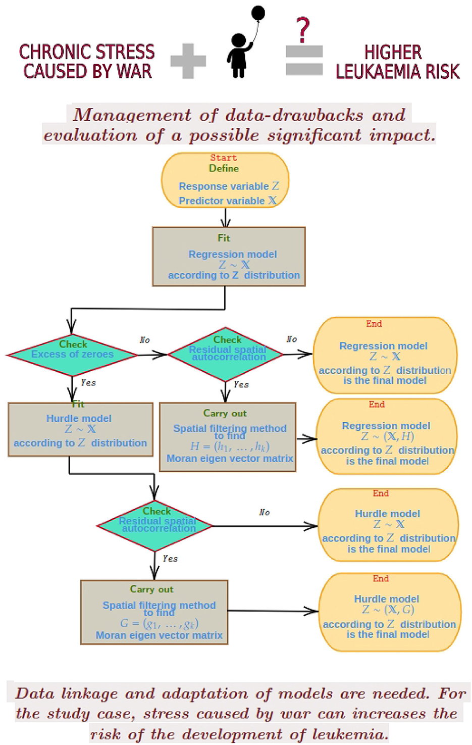
Figure 6. Summary of the methodological proposal, study-case hypothesis and main results. G and H represent the matrix with MEMs for the respective model.

3. Results

It is estimated that more than 7 million Colombian people have been affected, more than 5 million people have been victims of displacement between 1985 and 2012, and more than 200,000 people have died, 80% of them civilians [37]. However, the collection and processing of information were difficult due to the lack of political will regarding the official acknowledgment of this conflict and its consequences [38].

3.1. Data description

The National Department of Planning (DNP) computed the armed conflict index (IICA) based on data collected from 2002 to 2013 [39]. This index was based on six variables: Armed actions, homicides, kidnappings, anti-personnel mines, forced displacement, and cultivation of coca. During this period, there was an upsurge in violent actions due to the breakdown of the government's truce [38, 40].

Childhood cancer is one of the main causes of morbidity and mortality in the world and the most frequent neoplastic childhood pathology. Pediatric acute leukemia (LAP) is the type of cancer most common in children, with a worldwide incidence rate of 5 cases per 100,000 children between 0 and 19 years of age [41]. In Colombia, its incidence rate was 4.8 cases per 100,000 inhabitants for the period from 2007 to 2011 and the mortality rate was 2.2 deaths per 100,000 inhabitants [42]. In Colombia, cancer is the eleventh cause of mortality in children under 1 year of age and reached the third position in children under 5 years of age in 2015 [43]. Survival in developed countries exceeds 80% [44]. Nevertheless, in developing countries, survival is between 10 and 40% [45]. The mandatory leukemia registry began in 2008. Therefore, data used here correspond to children born throughout the years 2002–2013 having a diagnosis of leukemia in 2008–2016.

There were born 11.149.695 children between 2002 and 2013 in 1.124 Colombian municipalities. There were 4.775 children diagnosed with leukemia during 2008–2016, born in 2002–2013. The 45.7% were female, and 12.4% died of acute leukemia.

We aggregate all variables by municipalities, and we use data linkage at this level to create the dataset based on the following sources:

• From the National Institute of Health (INS) we obtained anonymized data of children born between 2002 and 2013 diagnosed with (or who died due to) LAP.

• From the National Administrative Department of Statistics (DANE) we obtained Unmet Basic Needs (UBN) and Percentage of health coverage (Coverage).

• From DANE - 2005 Colombia Census Data Geodatabase, we obtain the Percentage of people living in rural areas (Per_Rur). And

• From the National Department of Planning (DNP) we obtained the Colombian index of armed conflict (IICA).

3.2. Exploratory spatial analysis

This is an ecological analysis of the incidence and mortality rates of LAP, in terms of IICA and UBN of a retrospective cohort. Figure 5 shows the spatial distribution across the country of the variables involved in this study. We analyze spatial autocorrelation using empirical Bayes modification of the Moran Index for rate variables, LR and LMR, and Moran Index for the rest of the variables. Lee's statistics index is used [33], for testing spatial cross-correlation between incidence and mortality rates and potential explanatory variables IICA, UBN, percentages of health coverage, and rural population. We test statistical significance, using Monte Carlo simulation for global and local indicators of Spatial Association (LISA) indices, and we present the respective significance maps. All variables present 95%-significant spatial autocorrelation. The Moran coefficients results are: 0.140, 0.065, 0.666, 0.645, 0.384, and 0.282 for LR, LMR, UBN, IICA, Per_Rur, and Coverage, respectively.

3.3. Spatial Poisson-Hurdle model results

Spatial Poisson Hurdle regression models are used in both cases, for LR and LMR, due to the detected overdispersion through excess zeros, and spatial autocorrelation found. To ignore this situation and estimate inappropriate models such as Poisson models leads to incorrect inferences [25]. See results in Tables 1, 2 for LR and LMR, respectively. Note that Moran's eigenvectors (MEM) are used here as a proxy for spatial correlation and other variables that we are not able to measure but that are relevant, see Figure 7. The model parameter estimation is carried out via maximum likelihood, and the spatial autocorrelation structure is incorporated by including the first eigenvector in both models, given that the first one is the only one that results statistically significant as an explanatory variable. See Figure 8 for a comparison between observed and fitted values. The residuals are now spatially uncorrelated. Moran I test under randomization p-values are 0.2119 and 0.1458 for LR and LMR model residuals, respectively. Finally, there is a summary and a flowchart of the process in the following Figure 6.

TABLE 1

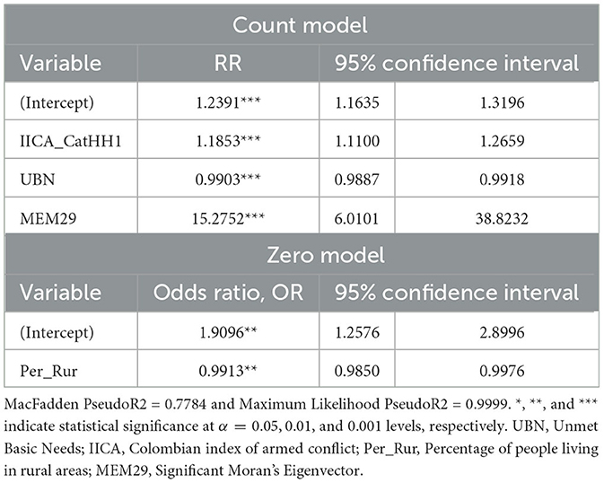
Table 1. Rate ratios with their respective 95% confidence intervals, obtained from the Poisson-Hurdle model fitted to the leukemia incidence rate.

TABLE 2

Table 2. Rate ratios with their respective 95% confidence intervals, obtained from the Poisson-hurdle model fitted to the leukemia mortality rate.

FIGURE 7

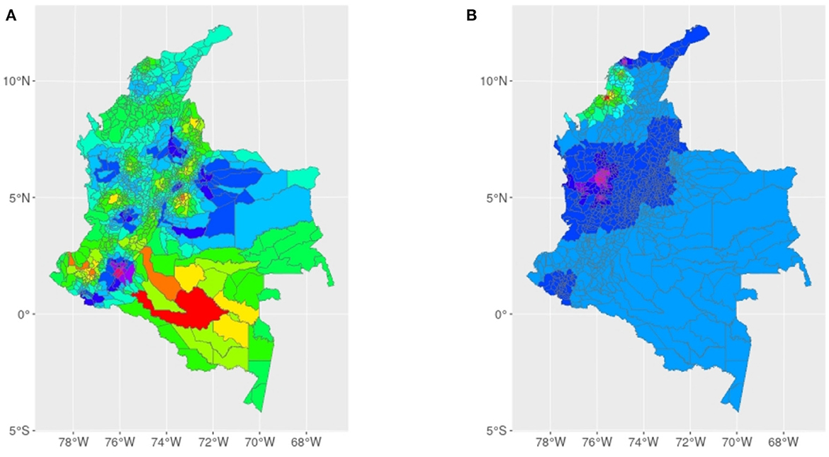
Figure 7. (A, B) Show the spatial distribution of the MEMs for LR y LMR, respectively. Both cases show positive spatial correlation, although correlation is stronger for the LMR case. The clusters are well-defined. The inclusion of this positive spatial association on the count model part, in both cases, also helps to explain variance. Now, there is no spatial autocorrelation or heterogeneity detected. MEMS increase from red, orange, and yellow for the lowest values, blues for the middle values, and the highest values become purple.

FIGURE 8

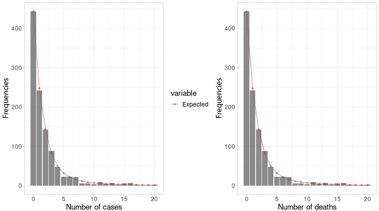
Figure 8. Comparison between empirical and fitted frequencies for incidence and mortality due to Leukemia. See fitted models in Tables 1, 2.

The computations in this paper are done using the free software R, and its packages spdep, rgeoda, sp, ggplot, pscl, and RANN. In most cases, pairwise distances and their functions are needed for the construction of the W matrix. So, N(N − 1)/2 distances have to be computed. The criteria use mainly Euclidean and nearest neighbors distances. For long distances, it is better to use a large circular distance because it considers the curvature, latitude, and longitude. Regarding the model, its estimation depends on the total of areal units, N, and the number of variables. The R packages have sets of internal parameters that control the computation issues, and have default values defined that usually work, sowhile the user can change them, this is rarely necessary. Given that we have only, 1124 area units and a few variables, the estimation of the models is not time-consuming. A recent complexity analysis of software to perform exploration of spatial data, including the packages, used here (spdep and rgeoda) among others, is presented in [46]. The rgeoda package is a modern implementation in R of a software for Windows called GeoDa, and has advantages in computational time for W matrix creation over spdep. However, spdep has truly important functionalities related to the estimation of spatial regression models and its implementation of Moran eigenvector filtering that makes this package more complete in this context.

Bivariate local indicator of spatial association shown in Figure 3, allows detecting areas with higher morbidity and mortality rates and higher IICA according to the DNP data: Catatumbo and the south of Cesar; Arauca; south of Bolívar; low Cauca antioqueño and Nudo of Paramillo; east Antioquia; south of Tolima and north of Cauca; Caucan Pacific, Tumaco, and Pacific Nariño; Ariari, Guayabero, and Guaviare; Caquetá and medium and low Putumayo. LM and LMR are spatially correlated with the peripheral border areas of the country, predominantly in the Orinoquia region and southern part of the Amazon, north of the Pacific and north of the Andean region, and the Caribbean toward Guajira. Of these regions, the involvement of 9 of the 15 zones of armed conflict described by the DNP stands out. There is no significant local or global spatial cross-correlation of leukemia incidence rate and rurality (global p = 0.2120). Mortality rates do not show significant spatial cross-correlation with rurality or health coverage, global p = 0.3510 and global p = 0.3390, respectively. LR and LMR variances exceed the mean.

A Poisson model on the data for each rate shows that with a confidence level of 95%, LR and LMR data are overdispersed, that is, true dispersion exceeds 1. According to Cameron and Trivedi overdispersion test [25], the results are: For LR, z = 4.1887 and p = 1.403e-05, and for LMR: z = 2.2049 and p = 0.01373. The excess of zeros is detected using the Score test for zero inflation [47], and p < 2.22e-16 for both rates. Comparing the observed frequency of zeroes in data with that predicted by generalized Poisson models, we have: For LR, 382 observed vs. 443 predicted, and for LMR 898 observed vs. 907 predicted. In addition, residuals of both generalized Poisson models are spatially autocorrelated according to Moran's Index test. Thus, we estimated Spatial Poisson Hurdle models described in Section 3.3 for LR as well as for LMR.

4. Discussion

This research shows how a prolonged armed conflict can impact the health of children. This fact is illustrated here using one of the most catastrophic conditions in childhood as is LAP. The association between armed conflict and pediatric acute leukemia has its conceptual basis in the epidemiology literature, given that, the incidence and mortality rates of neoplastic diseases increase with exposure to toxic and chronic stress during gestation and childhood.

Given that armed conflict and poverty are generators of ACEs we use them as explanatory variables of incidence and mortality of childhood leukemia rates. The measure used for armed conflict is the IICA and for poverty is the UBN. We found that the IICA is significant and positively correlated with both rates, so, it is a factor that increases the risk of childhood leukemia.

Contrary to expectations, the UBN is significant but negatively associated with both rates. This means that, according to the model results, a higher poverty level lowers childhood leukemia cases. However, this result could be a consequence of under-reporting data or miscounting from misdiagnosis. Thus, there are inaccurate records, if a child's diagnosis is malnutrition, infectious disease, or a late diagnosis.

These characteristics are also related to results found for the relationship between the percentage of rural population. This variable is significant and negative only for the zero-model part, in both cases: incidence and mortality. Thus, in both cases, the number of zeros observed is lower for municipalities with a higher proportion of rural areas. Basically, municipalities with people living in remote areas have an important problem of underreporting in data collection and late access to the health system.

In addition, for the mortality rate model, we include the percentage of health coverage as an explanatory variable. This predictor turns out to be significant only for the zero-model part, so, the higher the health coverage, the higher the number of observed zeros in the mortality from leukemia. The odds ratio estimated value emphasizes the relevance of access to professional and timely medical treatment. We want to draw attention to the fact that in developed countries, child mortality for this disease is almost null, while in low and middle-income countries like Colombia, the prognosis of cancer in children is poor due to delayed diagnoses and treatments, so, the provision of a children's cancer service is asymmetric and fragmented. Colombia has only 25 oncology service centers and half of them are in Bogotá, Antioquia, and Valle.

The novel combination of the Poisson-Hurdle model with the MEFS technique resulted in a simple and powerful methodology to deal with overdispersion, excess zeros, spatial autocorrelation, and spatial cross-correlation. Eigenvectors resulting from the MEFS method included as predictors gathered the spatial dependence and allowed valid models with non-correlated errors and with a good fit. Moreover, along with spatial dependence, eigenvectors also contain spatial effects of variables that were not possible to measure, such as ancestries, exposure to pesticides, closeness to illegal mining areas, access to education, and nutrition, among others. Prevention is urgently required. The study of exposure to toxic stress includes children, caregivers, environment, family strengthening and support networks, and political processes of peace and restoration. ACE prevention and trauma care diminish costs and reduce health inequality.

We hope that this research focuses attention on the importance of efforts to attain peace in Colombia, as well as the efforts to improve socio-economic conditions and thus build an equitable society.

Finally, we consider that mental and sociological health also can be seriously affected. Children suffer alterations in their upbringing, atypical social interactions, changes of behavior, and adaptation of the scale of values, to name a few. Type and access limitation to data, do not allow carrying on this study directly with individuals. However, it would be interesting to design a longitudinal study with a specific follow-up plan, at least for a small group of patients.

Dataset, Geographic Data Files, and R-code are attached as Supplementary material and also are freely available at https://github.com/mpbohorquezc/Spatial-Hurdle-models-Leukemia_armed_conflict.

Data availability statement

The original contributions presented in the study are included in the article/Supplementary material, further inquiries can be directed to the corresponding author.

Ethics statement

The studies involving humans were approved by Universidad Nacional de Colombia - Facultad de Medicina. The studies were conducted in accordance with the local legislation and institutional requirements. Written informed consent for participation in this study was provided by the participants' legal guardians/next of kin. Written informed consent was obtained from the individual(s) for the publication of any potentially identifiable images or data included in this article.

Author contributions

All authors listed have made a substantial, direct, and intellectual contribution to the work and approved it for publication.

Funding

This research was funded by the Universidad Nacional de Colombia and the Universidad Nacional abierta y a distancia (UNAD).

Conflict of interest

The authors declare that the research was conducted in the absence of any commercial or financial relationships that could be construed as a potential conflict of interest.

Publisher's note

All claims expressed in this article are solely those of the authors and do not necessarily represent those of their affiliated organizations, or those of the publisher, the editors and the reviewers. Any product that may be evaluated in this article, or claim that may be made by its manufacturer, is not guaranteed or endorsed by the publisher.

Supplementary material

The Supplementary Material for this article can be found online at: https://www.frontiersin.org/articles/10.3389/fams.2023.1150735/full#supplementary-material

References

1. Murray JS. Toxic stress and child refugees. J Special Pediatr Nurs. (2018) 23:e12200. doi: 10.1111/jspn.12200

PubMed Abstract | CrossRef Full Text | Google Scholar

2. Slopen N, Loucks EB, Appleton AA, Kawachi I, Kubzansky LD, Non AL, et al. Early origins of inflammation: an examination of prenatal and childhood social adversity in a prospective cohort study. Psychoneuroendocrinology. (2015) 51:403–13. doi: 10.1016/j.psyneuen.2014.10.016

PubMed Abstract | CrossRef Full Text | Google Scholar

3. Moyeda IXG, Sánchez BM, Cervantes DMO, Vega HAR. Relación entre maltrato fetal, violencia y sintomatología depresiva durante el embarazo de mujeres adolescentes y adultas: un estudio piloto. Psicologia y salud. (2013) 23:83–95. doi: 10.25009/pys.v23i1.518

CrossRef Full Text | Google Scholar

4. Cicchetti D, Hetzel S, Rogosch FA, Handley ED, Toth SL. An investigation of child maltreatment and epigenetic mechanisms of mental and physical health risk. Dev Psychopathol. (2016) 28:1305–17. doi: 10.1017/S0954579416000869

PubMed Abstract | CrossRef Full Text | Google Scholar

5. Furman D, Campisi J, Verdin E, Carrera-Bastos P, Targ S, Franceschi C, et al. Chronic inflammation in the etiology of disease across the life span. Nat Med. (2019) 25:1822–32. doi: 10.1038/s41591-019-0675-0

PubMed Abstract | CrossRef Full Text | Google Scholar

6. Fleming TP, Watkins AJ, Velazquez MA, Mathers JC, Prentice AM, Stephenson J, et al. Origins of lifetime health around the time of conception: causes and consequences. Lancet. (2018) 391:1842–52. doi: 10.1016/S0140-6736(18)30312-X

PubMed Abstract | CrossRef Full Text | Google Scholar

7. Paltiel O, Harlap S, Deutsch L, Knaanie A, Massalha S, Tiram E, et al. Birth weight and other risk factors for acute leukemia in the Jerusalem Perinatal Study cohort. Cancer Epidemiol Biomark Prev. (2004) 13:1057–64. doi: 10.1158/1055-9965.1057.13.6

PubMed Abstract | CrossRef Full Text | Google Scholar

8. Bandinelli LP, Levandowski ML, Grassi-Oliveira R. The childhood maltreatment influences on breast cancer patients: a second wave hit model hypothesis for distinct biological and behavioral response. Med Hypotheses. (2017) 108:86–93. doi: 10.1016/j.mehy.2017.08.007

PubMed Abstract | CrossRef Full Text | Google Scholar

9. Greaves M. Childhood leukaemia. BMJ. (2002) 324:283–7. doi: 10.1136/bmj.324.7332.283

CrossRef Full Text | Google Scholar

10. Krizanova O, Babula P, Pacak K. Stress, catecholaminergic system and cancer. Stress. (2016) 19:419–28. doi: 10.1080/10253890.2016.1203415

PubMed Abstract | CrossRef Full Text | Google Scholar

11. Anda RF, Butchart A, Felitti VJ, Brown DW. Building a framework for global surveillance of the public health implications of adverse childhood experiences. Am J Prev Med. (2010) 39:93–8. doi: 10.1016/j.amepre.2010.03.015

PubMed Abstract | CrossRef Full Text | Google Scholar

12. Danese A, McEwen BS. Adverse childhood experiences, allostasis, allostatic load, and age-related disease. Physiol Behav. (2012) 106:29–39. doi: 10.1016/j.physbeh.2011.08.019

PubMed Abstract | CrossRef Full Text | Google Scholar

13. Broyles ST, Staiano AE, Drazba KT, Gupta AK, Sothern M, Katzmarzyk PT. Elevated C-reactive protein in children from risky neighborhoods: evidence for a stress pathway linking neighborhoods and inflammation in children. PLoS ONE. (2012) 7:e45419. doi: 10.1371/journal.pone.0045419

PubMed Abstract | CrossRef Full Text | Google Scholar

14. Ports KA, Holman DM, Guinn AS, Pampati S, Dyer KE, Merrick MT, et al. Adverse childhood experiences and the presence of cancer risk factors in adulthood: a scoping review of the literature from 2005 to 2015. J Pediatr Nurs. (2019) 44:81–96. doi: 10.1016/j.pedn.2018.10.009

PubMed Abstract | CrossRef Full Text | Google Scholar

15. Bahri N, Fathi Najafi T, Homaei Shandiz F, Tohidinik HR, Khajavi A. The relation between stressful life events and breast cancer: a systematic review and meta-analysis of cohort studies. Breast Cancer Res Treat. (2019) 176:53–61. doi: 10.1007/s10549-019-05231-x

PubMed Abstract | CrossRef Full Text | Google Scholar

16. McDonald PG, Antoni MH, Lutgendorf SK, Cole SW, Dhabhar FS, Sephton SE, et al. A biobehavioral perspective of tumor biology. Discov Med. (2009) 5:544–7.

PubMed Abstract | Google Scholar

17. Steele A, Schubiger LI. Democracy and civil war: the case of Colombia. Conflict Manage Peace Sci. (2018) 35:587–600. doi: 10.1177/0738894218787780

CrossRef Full Text | Google Scholar

18. Maher D. Civil War and Uncivil Development: Economic Globalisation and Political Violence in Colombia and Beyond. 1st ed. Salford: Palgrave Macmillan (2018)

Google Scholar

19. Kadir A, Shenoda S, Goldhagen J. Effects of armed conflict on child health and development: a systematic review. PLoS ONE. (2019) 14:e0210071. doi: 10.1371/journal.pone.0210071

CrossRef Full Text | Google Scholar

20. Ospina-Alvarado M, Alvarado S, Carmona J, Ospina H. A social constructionist approach to understanding the experiences of girls affected by armed conflict in Colombia. In: Denov M, Akesson B, editors. Children Affected by Armed Conflict. Columbia University Press (2017). doi: 10.7312/deno17472-006

CrossRef Full Text | Google Scholar

21. Valencia-Suescun MI, Ramirez M, Fajardo MA, Ospina-Alvarado MC. From negative impacts to new possibilities: children in the Colombian armed. Revista Latinoamericana de Ciencias Sociales Ninez y Juventud. (2015) 13:1037–51. doi: 10.11600/1692715x.13234251114

CrossRef Full Text | Google Scholar

22. Hillis SD, Mercy JA, Saul JR. The enduring impact of violence against children. Psychol Health Med. (2017) 22:393–405. doi: 10.1080/13548506.2016.1153679

PubMed Abstract | CrossRef Full Text | Google Scholar

23. Korycinski RW, Tennant BL, Cawley MA, Bloodgood B, Oh AY, Berrigan D. Geospatial approaches to cancer control and population sciences at the United States cancer centers. Cancer Causes Control. (2018) 29:371–7. doi: 10.1007/s10552-018-1009-0

PubMed Abstract | CrossRef Full Text | Google Scholar

24. Ribeiro RC, Pui CH. Saving the children–improving childhood cancer treatment in developing countries. N Engl J Med. (2005) 352:2158–60. doi: 10.1056/NEJMp048313

CrossRef Full Text | Google Scholar

25. Cameron AC, Trivedi PK. Regression Analysis of Count Data. Cambridge University Press (2013). p. 597.

Google Scholar

26. Li Y, Shang Y, Yang Y. Clustering coefficients of large networks. Inform Sci. (2017) 382–3:350–8. doi: 10.1016/j.ins.2016.12.027

CrossRef Full Text | Google Scholar

27. Anselin L, Gallo JL, Jayet H. Spatial panel econometrics. In: Mátyás L, Sevestre P, editors. The Econometrics of Panel Data: Fundamentals and Recent Developments in Theory and Practice. Berlin; Heidelberg: Springer (2008). p. 625-60.

Google Scholar

28. Griffith DA, Peres-Neto PR. Spatial modeling in ecology: the flexibility of eigenfunction spatial analyses. Ecology. (2006) 87:2603–13. doi: 10.1890/0012-9658(2006)872603:SMIETF2.0.CO;2

PubMed Abstract | CrossRef Full Text | Google Scholar

29. Friendly M, Dray S, Guerry, BR. Maps, Data and Methods Related to Guerry (1833) Moral Statistics of France. CRAN (2023).

Google Scholar

30. Griffith DA, Chun Y. Implementing Moran eigenvector spatial filtering for massively large georeferenced datasets. Int J Geograph Inform Sci. (2019) 33:1703–17. doi: 10.1080/13658816.2019.1593421

CrossRef Full Text | Google Scholar

31. Moran PA. The interpretation of statistical maps. J R Stat Soc Ser B Methodol. (1948) 10:243–51.

Google Scholar

32. Lee SI. Developing a bivariate spatial association measure: an integration of Pearson's R and Moran's I. J Geograph Syst. (2001) 3:369–85. doi: 10.1007/s101090100064

CrossRef Full Text | Google Scholar

33. Hilbe JM. Modeling Count Data. Cambridge University Press (2014). p. 300.

Google Scholar

34. Zhang Y, Chen N, Du W, Yao S, Zheng X. A new geo-propagation model of event evolution chain based on public opinion and epidemic coupling. Int J Environ Res Public Health. (2020) 17:9235. doi: 10.3390/ijerph17249235

PubMed Abstract | CrossRef Full Text | Google Scholar

35. Galiana N, Barros C, Braga J, Ficetola GF, Maiorano L, Thuiller W, et al. The spatial scaling of food web structure across European biogeographical regions. Ecography. (2021) 44:653–64. doi: 10.1111/ecog.05229

PubMed Abstract | CrossRef Full Text | Google Scholar

36. Dray S, Legendre P, Peres-Neto PR. Spatial modelling: a comprehensive framework for principal coordinate analysis of neighbour matrices (PCNM). Ecol Modell. (2006) 196:483–93. doi: 10.1016/j.ecolmodel.2006.02.01510.15446/hys.n26.44516

CrossRef Full Text | Google Scholar

37. Cely DMF. Grupo de memoria histórica, ¡basta ya! Colombia: Memorias de guerra y dignidad (bogotá: Imprenta nacional, 2013), 431 pp. 1. Historia y sociedad. (2014) 274–81. doi: 10.15446/hys.n26.44516

CrossRef Full Text | Google Scholar

38. Calderón Rojas JC. Etapas del conflicto armado en Colombia: hacia el posconflicto. Latinoamérica Revista de Estudios Latinoamericanos (2016) 227–57. doi: 10.1016/j.larev.2016.06.010

CrossRef Full Text | Google Scholar

39. DNP. Indice de Incidencia del Conflicto Armado (2021). Available online at: www.dnp.gov.co (accessed March 4, 2021).

Google Scholar

40. Albert M. El conflicto en Colombia: ?es posible la paz (2004). Available online at: http://rua.ua.es/dspace/handle/10045/2740

Google Scholar

41. Milaniak I, Jaffee SR. Childhood socioeconomic status and inflammation: a systematic review and meta-analysis. Brain Behav Immunity. (2019) 78:161–76. doi: 10.1016/j.bbi.2019.01.018

PubMed Abstract | CrossRef Full Text | Google Scholar

42. de Oliveira MM, Silva DRM, Ramos FR, Curado MP. Children and adolescents cancer incidence, mortality and survival a population-based study in Midwest of Brazil. Cancer Epidemiol. (2020) 68:101795. doi: 10.1016/j.canep.2020.101795

PubMed Abstract | CrossRef Full Text | Google Scholar

43. Hansen C, Paintsil E. Infectious diseases of poverty in children: a tale of two worlds. Pediatr Clin. (2016) 63:37–66. doi: 10.1016/j.pcl.2015.08.002

PubMed Abstract | CrossRef Full Text | Google Scholar

44. Fabian ID, Abdallah E, Abdullahi SU, Abdulqader RA, Boubacar SA, Ademola-Popoola DS, et al. Global retinoblastoma presentation and analysis by national income level. JAMA Oncol. (2020) 6:685–95. doi: 10.1001/jamaoncol.2019.6716

PubMed Abstract | CrossRef Full Text | Google Scholar

45. Rodriguez-Villamizar LA, Rojas Díaz MP, Acuña Merchán LA, Moreno-Corzo FE, Ramírez-Barbosa P. Space-time clustering of childhood leukemia in Colombia: a nationwide study. BMC Cancer. (2020) 20:48. doi: 10.1186/s12885-020-6531-2

PubMed Abstract | CrossRef Full Text | Google Scholar

46. Anselin L, Li X, Koschinsky J. GeoDa, from the desktop to an ecosystem for exploring spatial data. Geograph Anal. (2022) 54:439–66. doi: 10.1111/gean.12311

CrossRef Full Text | Google Scholar

47. van den Broek J. A score test for zero inflation in a Poisson distribution. Biometrics. (1995) 51:738–43. doi: 10.2307/2532959

PubMed Abstract | CrossRef Full Text | Google Scholar