Accelerated non-negative tensor completion via integer programming

1. Introduction

A tensor is a multi-dimensional array or a generalized matrix. ψ is called an order-p tensor if $\psi \in {ℝ}^{r_1\times \cdots \times r_p}$, where r_i is the length of the i-th dimension of ψ. For example, an RGB image with a size of 30 by 30 pixels is an order-3 tensor in ℝ^{30 × 30 × 3}. Since tensors and matrices are closely related, many matrix problems can be naturally generalized to tensors, such as computing a matrix norm and decomposing a matrix. However, the tensor generalization of such problems can be substantially more computationally challenging [1].

Similar to matrix completion, tensor completion uses the observed entries of a partially observed tensor ψ to interpolate the missing entries with a restriction on the rank of the interpolated tensor. The purpose of the rank restriction is to restrict the degree of freedom of the missing entries [2], e.g., avoiding overfitting. Without this rank restriction, the tensor completion problem becomes ill-posed because there are too many degrees of freedom that need to be constrained by the available data. Tensor completion is a versatile model with many important applications in social sciences [3], healthcare [4], computer vision [5], and many other domains.

In the past decade, there have been major advances in matrix completion [6]. However, for general tensor completion, there remains a critical tension. Past approaches either have polynomial-time computation but require exponentially more samples than the information-theoretic rate [4, 7–9], or they achieve the information-theoretic rate but require solving NP-hard problems for which there are no known practical numerical algorithms [10–13].

We note that, aside from matrix completion, for some special cases of tensor completion, there are numerical algorithms that can achieve the information-theoretic rate; for instance, non-negative rank-1 [14] tensors, or orthogonal symmetric [15] tensors. In this study, we focus on a new approach, proposed by Bugg et al. [16], that is designed for entrywise-nonnegative tensors, which naturally exist in applications such as image demosaicing. The authors defined a new norm for non-negative tensors by using the gauge of a specific 0–1 polytope that they constructed. By using this gauge norm, their approach achieved the information-theoretic rate in terms of sample complexity although the resulting problem is NP-hard to solve. Nevertheless, a practical approach was attained: as the norm is defined by using a 0–1 polytope, the authors embedded integer linear optimization within the blended conditional gradients (BCG) algorithm [17], a variant of the Frank-Wolfe algorithm, to construct a numerical computation algorithm that required a linear (in numerical tolerance) number of oracle steps to converge to the global optimum.

This study proposes several acceleration techniques for the original numerical computation algorithm created by Bugg et al. [16]; we tested multiple techniques in combination to evaluate the configuration that provides the best overall speedup. The motivation is to further improve the implementation on large-scale problems. Our variants can maintain the same theoretical guarantees as the original algorithm while offering potential speedups. Indeed, our experiments demonstrate that such speedups can be attained consistently across a range of problem instances. Additionally, this study provides a full description of the original numerical computation algorithm and its coding implementation, details that were omitted in Bugg et al. [16].

We summarize preliminary material and introduce the framework and theory of Bugg et al. [16]'s non-negative tensor completion approach in Section 2. Then, we describe the computation algorithm of their approach in Section 3 and our acceleration techniques in Section 4. Numerical experiment results are presented in Section 5.

2. Preliminaries

Given an order-p tensor $\psi \in {ℝ}^{r_1\times \cdots \times r_p}$, we refer to its entry with indices x = (x₁, …, x_p) as ψ_x: = ψ_{x1, …, xp}. x_i∈[r_i] is the value of the i-th index, where [r_i]: = {1, …, r_i}. We also define $\rho :=\sum _i{r}_i$, π: = ∏_ir_i and $\mathcal{R}=\left[r_1\right]\times \cdots \times \left[r_p\right]$. The probability simplex ${\Delta }^k:=conv\left\{e_1,\dots ,e_k\right\}$ is the convex hull of the coordinate vectors in dimension k.

A nonnegative rank-1 tensor ψ is defined as ψ: = θ⁽¹⁾⊗⋯⊗θ^(p), where ${\theta }^{(k)}\in {ℝ}_{+}^{r_k}$ are non-negative vectors. Its entry ψ_x is ${\prod }_{k=1}^p{\theta }_{x_k}^{(k)}$. Bugg et al. [16] defined the ball of nonnegative rank-1 tensors whose maximum entry is λ∈ℝ₊ to be

$\begin{array}{ll}{\mathcal{B}}_{\lambda }=\{\psi :{\psi }_x=\lambda ·{\displaystyle \prod _{k=1}^p}{\theta }_{x_k}^{(k)},{\theta }_{x_k}^{(k)}\in \left[0,1\right],\text{for}x\in \mathcal{R}\},& (1)\end{array}$

so the nonnegative rank of nonnegative tensor is

$\begin{array}{ll}{rank}_{+}(\psi )=min\{q|\psi ={\displaystyle \sum _{k=1}^q}{\psi }^k,{\psi }^k\in {\mathcal{B}}_{\infty }\text{for}k\in \left[q\right]\},& (2)\end{array}$

where ${\mathcal{B}}_{\infty }=\underset{\lambda \to \infty }{lim}{\mathcal{B}}_{\lambda }$. For a λ∈ℝ₊, consider a finite set of points

$\begin{array}{ll}{\mathcal{S}}_{\lambda }=\{\psi :{\psi }_x=\lambda ·{\displaystyle \prod _{k=1}^p}{\theta }_{x_k}^{(k)},{\theta }_{x_k}^{(k)}\in \left\{0,1\right\},\text{for}x\in \mathcal{R}\}.& (3)\end{array}$

Bugg et al. [16] established the following connection between ${\mathcal{B}}_{\lambda }$ and ${\mathcal{S}}_{\lambda }$:

$\begin{array}{ll}{\mathcal{C}}_{\lambda }:=conv({\mathcal{B}}_{\lambda })=conv({\mathcal{S}}_{\lambda }),& (4)\end{array}$

where ${\mathcal{C}}_{\lambda }$ is the non-negative tensor polytope. Bugg et al. [16] also presented three implications of this result that are useful to their non-negative tensor completion approach. First, ${\mathcal{C}}_{\lambda }$ is a polytope. Second, the elements of ${\mathcal{S}}_{\lambda }$ are the vertices of ${\mathcal{C}}_{\lambda }$. Third, the following relationships hold: ${\mathcal{B}}_{\lambda }=\lambda {\mathcal{B}}_1$, ${\mathcal{S}}_{\lambda }=\lambda {\mathcal{S}}_1$, and ${\mathcal{C}}_{\lambda }=\lambda {\mathcal{C}}_1$.

2.1. Norm for non-negative tensors

Key to the theoretical guarantee and numerical computation of Bugg et al. [16]'s approach is their construction of a new norm for non-negative tensors using a gauge (or Minkowski functional) construction.

Definition 2.1 (Bugg et al. [16]). The function defined as

$\begin{array}{ll}||\psi {||}_{+}:=inf\left\{\lambda \ge 0|\psi \in \lambda {\mathcal{C}}_1\right\}& (5)\end{array}$

is a norm for nonnegative tensors $\psi \in {ℝ}_{+}^{r_1\times \cdots \times r_p}$.

This norm has an important property that it can be used as a convex surrogate for tensor rank [16]. In other words, if ψ is a non-negative tensor, then we have ||ψ||_max ≤ ||ψ||₊ ≤ rank₊(ψ)·||ψ||_max. If ||ψ||₊ = 1, then ||ψ||₊ = ||ψ||_max.

2.2. Non-negative tensor completion

For a partially observed order-p tensor ψ, let $(x\langle i\rangle ,y\langle i\rangle )\in \mathcal{R}\times ℝ$ for i = 1, …, n denote the indices and value of n observed entries. We assume that an entry can be observed multiple times, so let U: = {x〈1〉, …, x〈u〉}, where u ≤ n denote the set of unique indices of observed entries. Since ||·||₊ is a convex surrogate for tensor rank, we have the following non-negative tensor completion problems:

$\begin{array}{l}\widehat{\psi }\in \arg \underset{\psi }{\min }\frac{1}{n}{\displaystyle \sum _{i=1}^n{\left(y\langle i\rangle -{\psi }_{x\langle i\rangle }\right)}^2}\\ \text{ s}.\text{t}.\Vert \psi {\Vert }_{+}\le \lambda & (6)\end{array}$

where λ∈ℝ₊ is given and $\hat{\psi }$ is the completed tensor. The feasible set {ψ:||ψ||₊ ≤ λ} is equivalent to ${\mathcal{C}}_{\lambda }$ by the norm definition (2.1) and ${\mathcal{C}}_{\lambda }=\lambda {\mathcal{C}}_1$.

Although the problem (6) is a convex optimization problem, Bugg et al. [16] showed that solving it is NP-hard. Nonetheless, Bugg et al. [16] managed to design an efficient numerical computation algorithm of global minima of the problem (6) by using its substantial structure of the problem. We will explain their algorithm more after showing their findings on the statistical guarantees of the problem (6).

2.2.1. Statistical guarantees

Bugg et al. [16] observed that the problem (6) is equivalent to a convex aggregation [18–20] problem for a finite set of functions, so we have the following tight generalization bound for the solution of the problem (6)

Proposition 2.1 (Lecué [20]). Suppose |y| ≤ b almost surely. Given any δ>0, with probability at least 1 − 4δ we have that

$\begin{array}{ll}𝔼\left({(y-{\hat{\psi }}_x)}^2\right)\le {\displaystyle \underset{\phi \in C_{\lambda }}{min}}𝔼\left({(y-{\hat{\phi }}_x)}^2\right)+c_0·max\left[b^2,{\lambda }^2\right]·max\left[{\zeta }_n,\frac{log(1/\delta )}{n}\right],& (7)\end{array}$

where c₀ is an absolute constant and

$\begin{array}{ll}{\zeta }_n=\{\begin{array}{l}\frac{2^{\rho }}{n},if{2}^{\rho }\le \sqrt{n}\\ \sqrt{\frac{1}{n}\log \left(\frac{e{2}^{\rho }}{\sqrt{n}}\right)},if{2}^{\rho }>\sqrt{n}\end{array}& (8)\end{array}$

Under specific noise models such as an additive noise model, we have the following corollary to the above proposition combined with the fact that ||·||₊ is a convex surrogate for tensor rank.

Corollary 2.1 (Bugg et al. [16]). Suppose φ is a non-negative tensor with rank₊(φ) = k and ||φ||_max ≤ μ. If (x〈i〉, y〈i〉) are independent and identically distributed with |y|〈i〉−φ_x〈i〉 ≤ e almost surely and 𝔼y〈i〉 = φ_x〈i〉, then given any δ>0, with probability at least 1 − 4δ, we have

$\begin{array}{ll}𝔼\left({(y-{\hat{\psi }}_x)}^2\right)\le e^2+c_0·{(\mu k+e)}^2·max\left[{\zeta }_n,\frac{log(1/\delta )}{n}\right]& (9)\end{array}$

where ζ_n is as in (8) and c₀ is an absolute constant.

The two results above show that the problem (6) achieves the information-theoretic sample complexity rate when k = O(1).

3. Original computation algorithm

Since ${\mathcal{C}}_1$ is a 0–1 polytope, we can employ integer linear optimization to address the linear separation problem associated with this polytope. Thus, we can apply the Frank–Wolfe algorithm or its variants to solve the problem (6) to a desired numerical tolerance. Bugg et al. [16] choose the BCG variant for two reasons.

First, the BCG algorithm can terminate (within numerical tolerance) in a linear number of oracle steps for an optimization problem with a polytope feasible set and a strictly convex objective function over the feasible set. To make the objective function in the problem (6) strictly convex, we can reformulate the problem (6) by changing its feasible set from ${\mathcal{C}}_{\lambda }$ to ${\mathrm{\text{Proj}}}_U({\mathcal{C}}_{\lambda })$. The implementation of this reformulation is to simply discard the unobserved entries of ψ. Second, the weak-separation oracle in the BCG algorithm accommodates early termination of the associated integer linear optimization problem, which is formulated as follows:

$\begin{array}{l}\underset{{}_{\phi ,\theta }}{\min }\langle c,\phi -\psi \rangle \\ \text{s}.\text{t}.\lambda ·(1-p)+\lambda ·{\displaystyle \sum _{k=1}^p{\theta }_{x_k}^{(k)}}\le {\phi }_{x}x\in ℛ\\ 0\le {\phi }_x\le \lambda ·{\theta }_{x_k}^{(k)}k\in [p],x\in ℛ\\ {\theta }_{x_k}^{(k)}\in \{0,1\}k\in [p],x\in ℛ& (10)\end{array}$

The feasible set in the problem above is equivalent to ${\mathcal{S}}_{\lambda }$, and the linear constraints above are acquired from standard techniques in integer optimization [21, 22]. Bugg et al. [16] also deploy a fast alternating minimization heuristic to solve the weak-separation oracle to avoid (if possible) solving the problem (10) via integer programming oracle.

Next, we will fully describe the Python 3 implementation of the BCG algorithm adapted by Bugg et al. [16] to solve the problem (6) and its major computation components. This detailed account is vital as it will aid in our explanation of how to accelerate this algorithm in the subsequent sections. It also supplements the algorithm description omitted in Bugg et al. [16]. Their code is available from https://github.com/WenhaoP/TensorComp. For brevity, we do not explain the abstract frameworks of the adapted BCG (ABCG) or its major computation components here, but they can be found in Bugg et al. [16] and Braun et al. [17].

3.1. Adapted blended conditional gradients

The ABCG is implemented as the function nonten in original_nonten.py. The inputs are indices of observed entries (X), values of observed entries (Y), dimension (r), λ (lpar), and numerical tolerance (tol). The output is the completed tensor $\hat{\psi }$ (sol). There are three important preparation steps of ABCG. First, it reformulates the problem (6) by changing the feasible set from ${\mathcal{C}}_{\lambda }$ to ${\mathrm{\text{Proj}}}_U({\mathcal{C}}_{\lambda })$. Second, it normalizes the feasible set to ${\mathrm{\text{Proj}}}_U({\mathcal{C}}_1)$ and scales sol by λ at the end of ABCG. Third, it flattens the iterate (psi_q) and recovers the original dimension of sol at the end of ABCG.

We first build the integer programming problem (10) in Gurobi. The iterate is initialized as a tensor of ones; the active vertex set {v₁, …, v_k} (Pts and Vts) and the active vertex weight set {γ₁, …, γ_k} (lamb) are initialized accordingly. Vts stores the θ⁽ⁱ⁾'s for constructing each active vertex in Pts. {v₁, …, v_k} are all order-p tensors, but they are vectorized in the code. bestbd stores the best lower bound for the optimal objective value found so far. It is initialized as 0, a lower bound on the optimal objective value of problem (6). objVal stores the objective function value of the current iterate. m._gap stores half of the current primal gap estimate, the difference between objVal and the optimal objective function value [17].

The iteration procedure of BCG is implemented as a while loop. In each iteration, we first compute the gradient of the objective function with respect to the current iterate codec (lines 318–320). Then, we compute the dot products ({〈lpar*c, v₁〉, …, 〈lpar*c, v_k〉}) between the scaled gradient (lpar*c) and each active vertex, store them in pro, and use pro to find the away-step vertex (psi_a) and the Frank-Wolfe-step vertex (psi_f). Based on the test that compares 〈lpar*c, psi_a - psi_f〉 and m._gap, we either use the simplex gradient descent step (SiGD) or the weak-separation oracle step (LPsep) to find the next iterate. Since we initialize m._gap as +∞, we always solve the problem (10) to solve the weak-separation oracle in the first iteration. At the end of each iteration, we update objVal and bestbd. The iteration procedure stops when either the primal gap estimate (2*m._gap) or the largest possible primal gap objVal - bestbd is smaller than tol.

Figure 1 is a flowchart that generally explains the entire procedure of the ABCG.

FIGURE 1

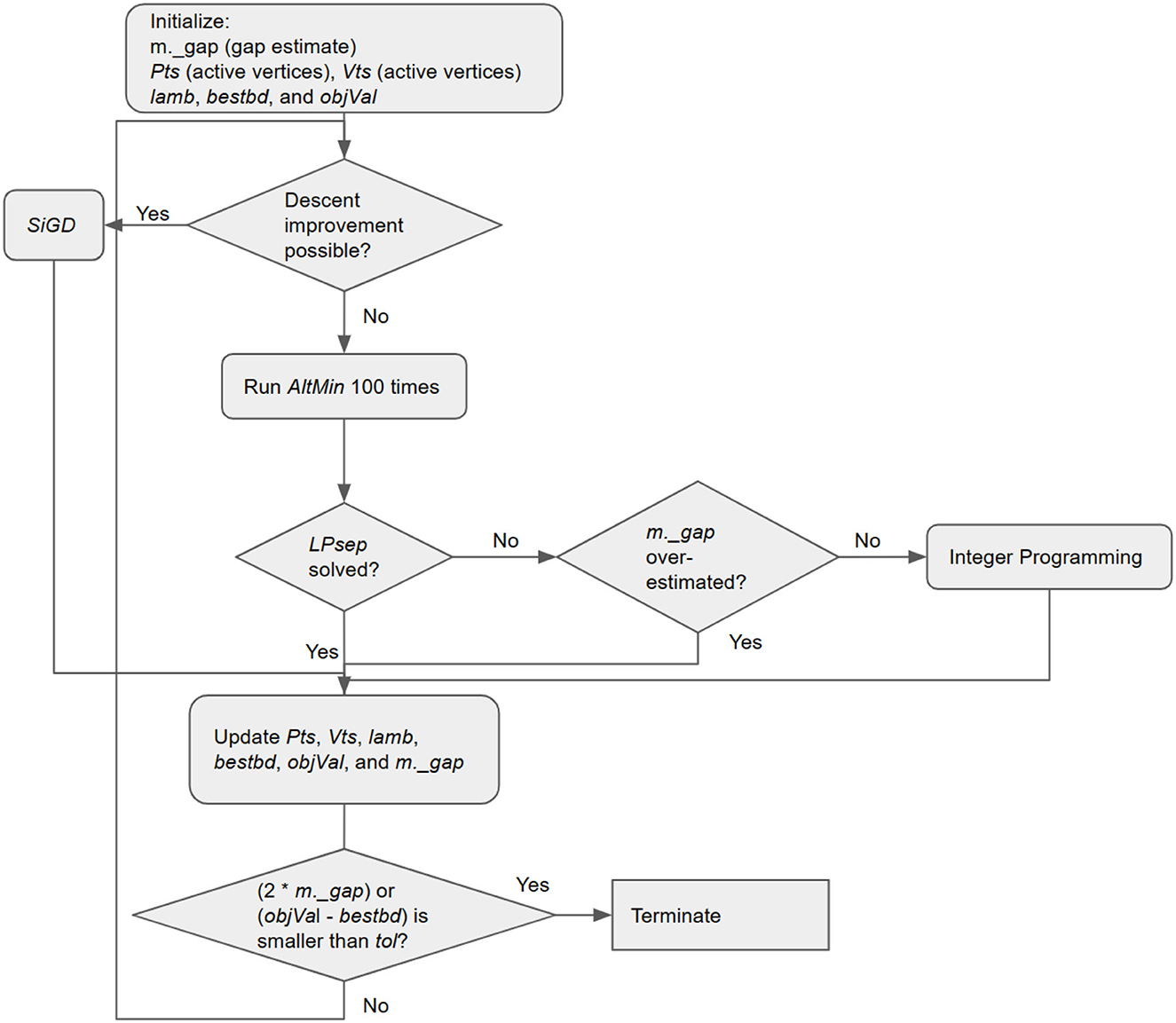
Figure 1. Flowchart of ABCG.

3.2. Simplex Gradient Descent Step

SiGD is implemented in the function nonten. It determines the next iterate with a lower objective function value via a single descent step that solves the following reformulation of the problem (6)

$\begin{array}{ll}\begin{array}{l}{\widehat{\gamma }}_1,\dots ,{\widehat{\gamma }}_k\in \arg \underset{{\gamma }_1,\dots ,{\gamma }_k\in {ℝ}_{+}}{\min }\frac{1}{n}{\displaystyle \sum _{j=1}^n(y\langle i\rangle }-({\displaystyle \sum _{j=1}^k{\gamma }_j{v}_j})x\langle i\rangle {)}^2\hfill \\ \text{ s.t. }{\displaystyle \sum _{j=1}^k{\gamma }_j}=1\hfill \end{array}& (11)\end{array}$

For clarity, we ignore the projection in the problem above. Since lamb is in Δ^k as all its elements are non-negative and sum to one, SiGD has the term “Simplex” in its name [17].

We first compute the projection of pro onto the hyperplane of Δ^k and store it in d. If all elements of d are zero, then we set the next iterate to the first active vertex and end SiGD. Otherwise, we solve the optimization problem $\widehat{\eta }=argmax\left\{\eta \in {ℝ}_{+}:\gamma -\eta d\ge 0\right\}$, where γ is lamb and d is d, and store the optimal solution $\widehat{\eta }$ in eta. Next, we compute psi_n which is $x-\widehat{\eta }\sum _i{d}_i{v}_i$ where x is the current iterate, d_i's are the elements of d, and v_i are active vertices. If the objective function value of psi_n is smaller or equal to that of the current iterate, then we set the next iterate to psi_n and drop any active vertex with zero weight in the updated active vertex set for constructing psi_n. This is called drop step in Braun et al. [17]. Otherwise, we perform an exact line search over the line segment between the current iterate and psi_n and set the next iterate to the optimal solution. This is called descent step in Braun et al. [17].

3.3. Weak-separation oracle step

LPsep is implemented in the function nonten. It has two differences from its implementation in the original BCG. First, whether it finds a new vertex that satisfies the weak-separation oracle or not, it always performs an exact line search over the line segment between the current iterate and that new vertex to find the next iterate. Second, it uses bestbd to update m._gap.

m._cmin is the dot product between lpar*c and the current iterate. The flag variable oflg is True if an improving vertex has not been found that satisfies either the weak-separation oracle or the conditions described below. We first repeatedly use the alternating minimization heuristic (AltMin) to solve the weak-separation oracle. If AltMin fails to do so within 100 repetitions but finds a vertex that shows that m._gap is an overestimate, we claim that it satisfies the weak-separation oracle and update m._gap. Otherwise, we solve the integer programming problem (10) via the Gurobi global solver to obtain a satisfying vertex and update m._gap. Note that an exact solution is not required; any solution attaining weak separation suffices.

3.4. Alternating minimization

AltMin is implemented as the function altmin in original_nonten.py. Since a vertex is in ${\mathcal{S}}_{\lambda }$, the objective function in the integer programming problem (10) becomes 〈c, (θ⁽¹⁾⊗⋯⊗θ^(p))−ψ〉, where ${\theta }^{(k)}\in {\left\{0,1\right\}}^{r_k}$. There is a motivating observation for solving this problem. For example, if we fix θ⁽²⁾, …, θ^(p), then the problem (10) is equivalent to $\underset{{\theta }^{(1)}\in {\left\{0,1\right\}}^{r_1}}{min}\langle {\tilde{c}}^{(1)},{\theta }^{(1)}\rangle$ where $\tilde{c}$ is a constant in ${ℝ}^{r_1}$ computed from c, θ⁽²⁾, …, θ^(p). The optimal solution can be easily found based on the signs of $\tilde{c}$'s entries as θ⁽¹⁾ is binary. AltMin utilizes this observation.

Given an incumbent solution ${\Theta }_0:=\left\{{\widehat{\theta }}_0^{(1)},\dots ,{\widehat{\theta }}_0^{(p)}\right\}$, AltMin keeps solving sequences of optimization problems to get Θ₁, Θ₂, …, Θ_T. For t = 1, …, T, we have

$\begin{array}{l}{\Theta }_t=\{{\widehat{\theta }}_t^{(1)}=\arg \underset{{\theta }_t^{(1)}\in {\{0,1\}}^{r_1}}{\min }\langle {\tilde{c}}_t^{(1)},{\theta }_t^{(1)}\rangle ,\dots ,{\widehat{\theta }}_t^{(p)}\\ =\arg \underset{{\theta }_t^{(p)}\in {\{0,1\}}^{r_p}}{\min }\langle {\tilde{c}}_t^{(p)},{\theta }_t^{(p)}\rangle \},& (12)\end{array}$

where ${\tilde{c}}_t^{(k)}$ stores in the variable fpro. At each t, ${\widehat{\theta }}_t^{(1)},\dots ,{\widehat{\theta }}_t^{(p)}$ are computed one by one. The difference between the objective function values in (10) of Θ_T−1 and Θ_T are guaranteed to be smaller than tol. AltMin outputs Θ_T at the end.

4. Accelerated computation algorithm

To show the efficacy and scalability of their approach, Bugg et al. [16] conducted numerical experiments on a personal computer. They compared the performance of their approach and three other approaches—alternating least squares (ALS) [23], simple low rank tensor completion (SiLRTC) [5], and trace norm regularized CP decomposition (TNCP) [2]—in four sets of different non-negative tensor completion problems. Normalized mean squared error (NMSE) $\left|\right|\hat{\psi }-\psi |{|}_F^2/|\left|\psi \right|{|}_F^2$ is used to measure the accuracy.

The results of their numerical experiments show that Bugg et al. [16]'s approach has higher accuracy but requires more computation time than the three other approaches in all four problem sets. We worked directly on their code base to design acceleration techniques. In addition to basic acceleration techniques such as caching repetitive computation operations, we designed five different acceleration techniques based on profiling results. By combining these five techniques differently, we created 10 variants of ABCG that can maintain the same theoretical guarantees but offer potentially faster computation.

4.1. Technique 1A: Index

The first technique, Index, accelerates AltMin. We initially computed fpro using a for-loop with u iterations, which can become time-consuming for large u (that is, large sample sizes). To address this, we rewrote the pro computation to use a for-loop with r_k iterations for k = 1, …, p. Despite each iteration in the new computation being more time-consuming than in the original, our numerical experiments showed a significant decrease in total computation time, particularly for problems with large sample sizes.

4.2. Technique 1B: Pattern

The second technique, Pattern, accelerates AltMin and builds upon the Index technique described above. Instead of extracting information from U during each iteration of the new loop operation in Index, we can extract it at the beginning of the algorithm since U remains unchanged throughout. This approach circumvents unnecessary repetition.

4.3. Technique 2: Sparse

The third technique, Sparse, accelerates the test that decides whether to use SiGD or LPsep for determining the next iterate. At the beginning of each BCG iteration, Pts and lpar*c are used to find psi_a and psi_f. This operation involves a matrix multiplication between Pts and lpar*c, which is time-consuming when Pts has a large size (i.e., large sample size or active vertex set size). We observed that the sparsity of Pts as vertices are binary and used a SciPy [24] sparse matrix to represent it instead of a NumPy [25] array. It not only accelerates the matrix multiplication but also reduces the memory usage for storing Pts.

4.4. Technique 3: NAG

The fourth technique NAG is for accelerating SiGD. Since SiGD is a gradient descent method, we can use Nesterov's accelerated gradient (NAG) to accelerate it. Specifically, we applied Besançon et al.'s [26] technique of transforming the problem (6) to its barycentric coordinates so that we minimize over Δ^k instead of the convex hull of the active vertex set. We restart the NAG when the active vertex set changes.

4.5. Technique 4: BPCG

The fifth technique BPCG is for accelerating SiGD. Tsuji et al. [27] developed the blended pairwise conditional gradients (BPCG) by combining the pairwise conditional gradients (PCG) with the blending criterion from BCG. Specifically, we applied the lazified version of BPCG, which only differs from BCG by replacing SiGD with PCG.

4.6. Computation variants

We have developed ten computational variants of ABCG by combining the five acceleration techniques described above. Further details about these variants are provided in Table 1 of Appendix 1. There are two observations. First, Index and Pattern are always used together as Pattern relies on Index, so we combine and consider them as a single technique in all following discussions. Second, NAG and BPCG are exclusive to each other as BPCG removes SiGD completely.

5. Numerical experiments

For benchmarking, we adopted the same problems (four sets of nonnegative tensor completion problems) and setup as Bugg et al. [16]. We repeated each problem 100 times. For each problem, we constructed the true tensor ψ by randomly choosing 10 points from ${\mathcal{S}}_1$ and then taking a random convex combination [16]. We conducted the experiments on a laptop equipped with 32GB of RAM and a 2.2Ghz Intel Core i7 processor with 6-cores/12-threads. The algorithms were coded in Python 3. Gurobi v9.5.2 [28] was used to solve the integer programming problem (10). The code is available from https://github.com/WenhaoP/TensorComp. We noted that the experiments in Bugg et al. [16] were conducted using a laptop computer with 8GB of RAM and an Intel Core i5 2.3Ghz processor with 2-cores/4-threads, algorithms coded in Python 3, and Gurobi v9.1 [28] to solve the integer programming problem (10).

We used NMSE to measure the accuracy and recorded its arithmetic mean (with its standard error) over 100 repetitions of each problem instance. We recorded the arithmetic mean (with its standard error), geometric mean, minimum, median, and maximum of the computation time over 100 repetitions of each problem instance. Generally speaking, the most effective variants were version 1 (Index + Pattern) and version 8 (BPCG + Index + Pattern), offering consistent speedups over the original version 0 (ABCG). All variants achieve almost the same NMSE as the original algorithm for each problem, which shows that they maintain in practice the same theoretical guarantee as the original algorithm; moreover, their runtimes were mostly competitive with the original.

5.1. Experiments with order-3 tensors

The first set of problems is order-3 tensors with increasing dimensions and n = 500 samples (with indices sampled with replacement). The results are shown in Table 2 of Appendix 2, and the arithmetic mean and median computation time are plotted in Figure 2. Among all versions, version 1 (Index + Pattern) has the lowest mean and median computation time for each problem except for the 100 × 100 × 100 tensor problem, where the original version 0 (ABCG) is slightly faster. Thus, we claim version 1 (Index + Pattern) as the best to use for this set of problems.

FIGURE 2

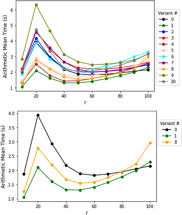
Figure 2. Results for order-3 non-negative tensors with size r × r × r and n = 500 samples.

5.2. Experiments with increasing tensor order

The second set of problems is tensors with an increasing tensor order, with each dimension r_i = 10 for i = 1, …, p, and n = 10, 000 samples. The results are in Table 3 of Appendix 2, and the arithmetic mean and median computation time is plotted in Figure 3. Among all the versions, version 1 (Index + Pattern) and version 8 (BPCG + Index + Pattern) has the lowest mean and median computation time for each problem except for the 10^×8 tensor problem. Thus, we claim versions 1 (Index + Pattern) and 8 (BPCG + Index + Pattern) are the best to use for this set of problems.

FIGURE 3

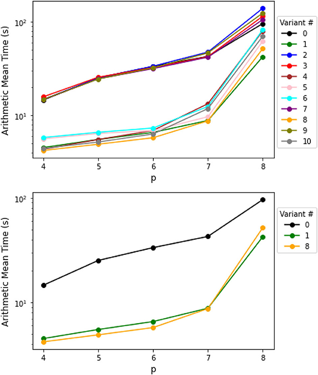
Figure 3. Results for increasing order non-negative tensors with size 10^×p and n = 10, 000 samples.

For the 10^×8 tensor problem, version 5 (NAG + Index + Pattern) has the lowest median computation time. We noted that the median computation time for this variant was significantly lower than the mean computation time, a trend also seen with other variants incorporating NAG. The maximum computation time of these versions is also much higher than other versions. This is due to the fact that, in certain cases, AltMin failed to solve the weak-separation oracle, and the Gurobi solver was needed to solve the time-consuming integer programming problem (10).

5.3. Experiments with increasing sample size

The third and fourth set of problems is tensors of size 10^×6 and 10^×7 with increasing sample sizes. The results are shown in Tables 4, 5 of Appendix 2, and the arithmetic mean and median computation time are plotted in Figures 4, 5. Among all the versions, either version 1 (Index + Pattern) or version 8 (BPCG + Index + Pattern) has the lowest mean and median computation time for each problem. Thus, we claim versions 1 (Index + Pattern) and 8 (BPCG + Index + Pattern) are the best to use for this set of problems.

FIGURE 4

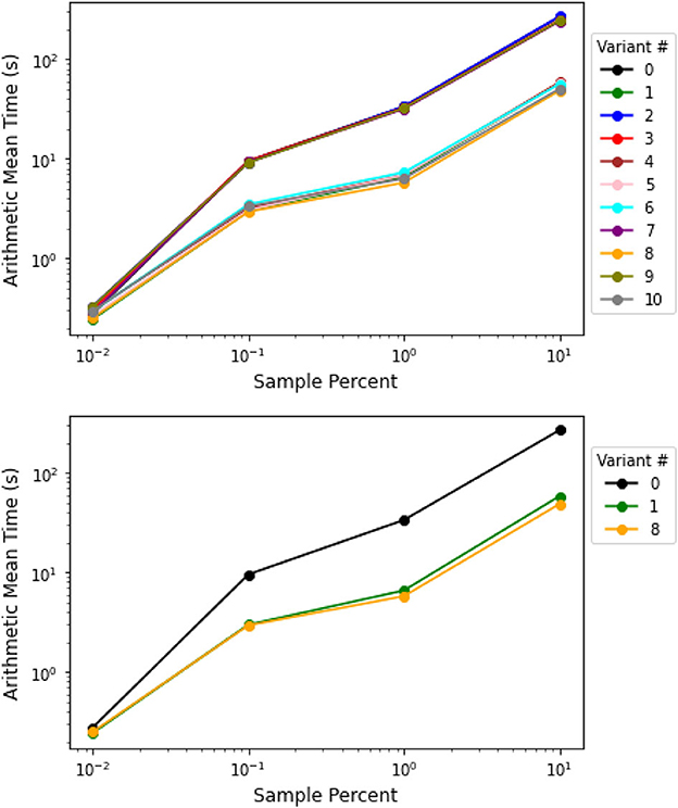
Figure 4. Results for non-negative tensors with size 10^×6 and increasing n samples.

FIGURE 5

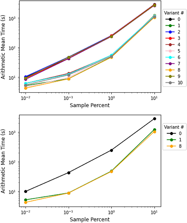
Figure 5. Results for non-negative tensors with size 10^×7 and increasing n samples.

6. Discussion and conclusion

In this study, we proposed and evaluated a range of speedup techniques for the original numerical computation algorithm for non-negative tensor completion, which was initially developed by Bugg et al. [16]. We benchmarked these algorithm variants on the same set of problem instances designed by Bugg et al. [16]. Our benchmarking results were that versions 1 (Index + Pattern) and 8 (BPCG + Index + Pattern) generally had the fastest computation time for solving the non-negative tensor completion problem (6), offering substantial speedups over the original algorithm. Version 1 had Index and Pattern techniques, and version 8 had BPCG, Index, and Pattern techniques. Because version 8 is version 1 with BPCG, version 8 may be preferred over version 1 for problem instances where the active vertex set could be large. Surprisingly, we found that Sparse failed to yield improvements. A possible reason is that the implementation of Sparse needs extra operations (e.g., finding the indices of nonzero entries) for converting NumPy arrays to SciPy sparse arrays. If the active vertex set is not large enough so that extra operations take time as least as the time saved from matrix multiplications of the active vertex set, then we cannot see an improvement. These results suggest that Index and Pattern are the most important for acceleration and that BCG and BPCG work equally well overall.

Data availability statement

The datasets presented in this study can be found in online repositories. The names of the repository/repositories and accession number(s) can be found at: https://github.com/WenhaoP/TensorComp.

Author contributions

WP, AA, and CC contributed to the conception and design of the study. WP did the programming, ran the numerical experiments, analyzed the results, and wrote the first draft of the manuscript. All authors contributed to the manuscript revision, read, and approved the submitted version.

Funding

This material was based upon work partially supported by the NSF under grant CMMI-1847666.

Conflict of interest

The authors declare that the research was conducted in the absence of any commercial or financial relationships that could be construed as a potential conflict of interest.

Publisher's note

All claims expressed in this article are solely those of the authors and do not necessarily represent those of their affiliated organizations, or those of the publisher, the editors and the reviewers. Any product that may be evaluated in this article, or claim that may be made by its manufacturer, is not guaranteed or endorsed by the publisher.

Supplementary material

The Supplementary Material for this article can be found online at: https://www.frontiersin.org/articles/10.3389/fams.2023.1153184/full#supplementary-material

References

1. Hillar CJ, Lim LH. Most tensor problems are NP-hard. J ACM. (2013) 60:1–39. doi: 10.1145/2512329

CrossRef Full Text | Google Scholar

2. Song Q, Ge H, Caverlee J, Hu X. Tensor completion algorithms in big data analytics. ACM Trans Knowl Discov Data. (2019) 13:1–48. doi: 10.1145/3278607

CrossRef Full Text | Google Scholar

3. Tan H, Wu Y, Feng G, Wang W, Ran B. A new traffic prediction method based on dynamic tensor completion. Procedia-Soc Behav Sci. (2013) 96:2431–42. doi: 10.1016/j.sbspro.2013.08.272

CrossRef Full Text | Google Scholar

4. Gandy S, Recht B, Yamada I. Tensor completion and low-n-rank tensor recovery via convex optimization. Inverse Probl. (2011) 27:025010. doi: 10.1088/0266-5611/27/2/025010

PubMed Abstract | CrossRef Full Text | Google Scholar

5. Liu J, Musialski P, Wonka P, Ye J. Tensor completion for estimating missing values in visual data. IEEE Trans Pattern Anal Mach Intell. (2013) 35:208–20. doi: 10.1109/TPAMI.2012.39

PubMed Abstract | CrossRef Full Text | Google Scholar

6. Zhang X, Wang D, Zhou Z, Ma Y. Robust low-rank tensor recovery with rectification and alignment. IEEE Trans Pattern Anal Mach Intell. (2019) 43:238–55. doi: 10.1109/TPAMI.2019.2929043

PubMed Abstract | CrossRef Full Text | Google Scholar

7. Mu C, Huang B, Wright J, Goldfarb D. Square deal: lower bounds and improved relaxations for tensor recovery. In: International Conference on Machine Learning. Cambridge, MA: PMLR. (2014). p. 73–81.

Google Scholar

8. Barak B, Moitra A. Noisy tensor completion via the sum-of-squares hierarchy. In: Conference on Learning Theory. Cambridge, MA: PMLR. (2016). p. 417–45.

PubMed Abstract | Google Scholar

9. Montanari A, Sun N. Spectral algorithms for tensor completion. Commun Pure Appl Math. (2018) 71:2381–425. doi: 10.1002/cpa.21748

CrossRef Full Text | Google Scholar

10. Chandrasekaran V, Recht B, Parrilo PA, Willsky AS. The convex geometry of linear inverse problems. Found Comput Math. (2012) 12:805–49. doi: 10.1007/s10208-012-9135-7

CrossRef Full Text | Google Scholar

11. Yuan M, Zhang CH. On tensor completion via nuclear norm minimization. Found Comput Math. (2016) 16:1031–68. doi: 10.1007/s10208-015-9269-5

CrossRef Full Text | Google Scholar

12. Yuan M, Zhang CH. Incoherent tensor norms and their applications in higher order tensor completion. IEEE Trans Inf Theory. (2017) 63:6753–66. doi: 10.1109/TIT.2017.2724549

CrossRef Full Text | Google Scholar

13. Rauhut H. Stojanac Ž. Tensor theta norms and low rank recovery. Numer Algorithms. (2021) 88:25–66. doi: 10.1007/s11075-020-01029-x

CrossRef Full Text | Google Scholar

14. Aswani A. Low-rank approximation and completion of positive tensors. SIAM J Matrix Anal Appl. (2016) 37:1337–64. doi: 10.1137/16M1078318

PubMed Abstract | CrossRef Full Text | Google Scholar

15. Rao N, Shah P, Wright S. Forward-backward greedy algorithms for atomic norm regularization. IEEE Trans Signal Process. (2015) 63:5798–811. doi: 10.1109/TSP.2015.2461515

CrossRef Full Text | Google Scholar

16. Bugg CX, Chen C, Aswani A. Nonnegative tensor completion via integer optimization. In:Oh AH, Agarwal A, Belgrave D, Cho K, , editors. Advances in Neural Information Processing Systems. San Diego, CA: Neural Information Processing Systems Foundation, Inc (NeurIPS) (2022). p. 10008–20.

Google Scholar

17. Braun G, Pokutta S, Tu D, Wright S. Blended conditonal gradients. In: International Conference on Machine Learning. PMLR. (2019). p. 735–43.

Google Scholar

18. Nemirovski A. Topics in non-parametric statistics. Lectures on Probability Theory and Statistics (Saint-Flour, 1998). Berlin: Springer (2000) 1738:85–277.

Google Scholar

19. Tsybakov AB. Optimal rates of aggregation. In:Schölkopf B, Warmuth MK, , editors. Learning Theory and Kernel Machines. Berlin: Springer (2003). p. 303–13. doi: 10.1007/978-3-540-45167-9_23

CrossRef Full Text | Google Scholar

20. Lecué G. Empirical risk minimization is optimal for the convex aggregation problem. Bernoulli. (2013) 19(5B):2153–66. doi: 10.3150/12-BEJ447

CrossRef Full Text | Google Scholar

21. Hansen P. Methods of nonlinear 0–1 programming. In:Hammer PL, Johnson EL, Korte BH, , editors. Annals of Discrete Mathematics, Vol. 5. Amsterdam: Elsevier (1979). p. 53–70. doi: 10.1016/S0167-5060(08)70343-1

CrossRef Full Text | Google Scholar

22. Padberg M. The Boolean quadric polytope: some characteristics, facets and relatives. Math Program. (1989) 45:139–72. doi: 10.1007/BF01589101

CrossRef Full Text | Google Scholar

23. Kolda TG, Bader BW. Tensor decompositions and applications. SIAM Rev. (2009) 51:455–500. doi: 10.1137/07070111X

CrossRef Full Text | Google Scholar

24. Virtanen P, Gommers R, Oliphant TE, Haberland M, Reddy T, Cournapeau D, et al. SciPy 10: fundamental algorithms for scientific computing in Python. Nat Methods. (2020) 17:261–72.

Google Scholar

25. Harris CR, Millman KJ, Van Der Walt SJ, Gommers R, Virtanen P, Cournapeau D, et al. Array programming with NumPy. Nature. (2020) 585:357–62. doi: 10.1038/s41586-020-2649-2

PubMed Abstract | CrossRef Full Text | Google Scholar

26. Besançon Besançon M, Carderera A, Pokutta S. FrankWolfe. jl: a high-performance and flexible toolbox for Frank-Wolfe algorithms and conditional gradients. INFORMS J Comput. (2022) 34:2611–20. doi: 10.1287/ijoc.2022.1191

CrossRef Full Text | Google Scholar

27. Tsuji K, Tanaka K, Pokutta S. Sparser kernel herding with pairwise conditional gradients without swap steps. arXiv. [preprint]. doi: 10.48550/arXiv.2110.12650

CrossRef Full Text | Google Scholar

28. Gurobi Optimization, LLC. Gurobi Optimizer Reference Manual. (2022). Beaverton, OR: Gurobi Optimization, LLC.

Google Scholar