Structure-preserving model reduction for port-Hamiltonian systems based on separable nonlinear approximation ansatzes

1. Introduction

In applications where multi-query evaluations of a computational model are required, such as optimization, control, or uncertainty quantification, model order reduction (MOR) techniques provide a powerful tool for accelerating the overall procedure, while maintaining an acceptable model accuracy. For a general overview of such methods, we refer to [1–5]. While most MOR techniques are based on a linear approximation of the full-order model (FOM) state, recently, methods based on nonlinear approximation ansatzes have received more and more attention, cf. [6–11] and the references therein. One reason for the great interest in the latter class of methods is that MOR methods based on linear approximation ansatzes are often inadequate for an effective reduction of transport-dominated systems, see for instance [12].

While nonlinear MOR techniques may lead to very low-dimensional and still accurate reduced-order models (ROMs), they do in general not guarantee that the ROM inherits important system properties of the corresponding FOM, such as stability. This may lead to unphysical behavior of the ROM or to approximation errors which grow exponentially with respect to time. In fact, the same issue also applies to most linear MOR methods and, thus, several MOR techniques have been proposed which preserve certain qualitative properties of the FOM [cf. [13–20]]. In this paper, we are especially interested in structure-preserving MOR methods for port-Hamiltonian (pH) systems, since these come with many desirable properties, cf. [21–23] for a general overview. For instance, a pH structure implies passivity and often also stability of the dynamical system. In addition, pH structures are closed under power-preserving interconnection, which makes them especially attractive for control purposes [24–27] and for modeling networks [28, 29]. Besides, since the energy plays the central role in the pH framework, it is suitable for a wide range of applications [30–41] as well as for the coupling of different physical domains [42–46].

The literature on structure-preserving MOR techniques for pH systems is mainly focused on linear time-invariant systems and using a linear approximation ansatz. Common techniques are based on balanced truncation [47–50] or transfer function interpolation [51–55]. Aside from these projection-based techniques, also direct optimization approaches have been proposed for obtaining a port-Hamiltonian ROM [cf. [56, 57]]. In [58], the authors present a structure-preserving MOR approach for nonlinear pH systems using a linear approximation ansatz based on the proper orthogonal decomposition (POD) or the iterative rational Krylov algorithm presented in [59]. In addition, they propose a structure-preserving variant of the discrete empirical interpolation method, which has been originally introduced in [60] and enables an efficient evaluation of the ROM.

While the contributions mentioned in the previous paragraph are all based on linear approximation ansatzes, we present in this paper a structure-preserving MOR approach for a special class of nonlinear pH systems based on suitable nonlinear approximation ansatzes, cf. section 2 for the details. The main contributions are listed in the following.

• We present a structure-preserving MOR approach using suitable nonlinear approximation ansatzes which are especially relevant in the context of transport-dominated systems. Especially, this approach is not limited to linear systems, but may be applied to a special class of nonlinear pH systems [cf. Theorem 4.3 (1)].

• We demonstrate that, in a special case which includes linear port-Hamiltonian FOMs with non-degenerate Hamiltonian, the approach allows to obtain ROMs which are at the same time pH and optimal in terms of residual minimization [cf. Theorem 4.3 (2)].

• We provide sufficient conditions which ensure that the state equations of the port-Hamiltonian ROMs with vanishing input signal are stable in the sense that the first block component of the ROM state as well as the resulting approximation of the FOM state are bounded [cf. Corollary 4.5].

• We present a new pH representation of a wildland fire model which has been considered for example in [61, 62] [cf. section 5.3].

The remainder of this manuscript is structured as follows. In section 2, we briefly introduce the mathematical setting considered in this paper by introducing the treated classes of pH systems and approximation ansatzes. We proceed by providing some preliminary definitions and results in section 3 with particular focus on differential equations, pH systems, and MOR. The main results are presented in section 4 where we especially demonstrate how to achieve structure-preserving MOR for pH systems based on special nonlinear approximation ansatzes. Finally, we illustrate the theoretical results by means of two numerical test cases in section 5 and provide a summary and an outlook in section 6.

1.1. Notation

The set of real numbers is denoted with ℝ and we use ℝ^{m, n} for the set of m×n matrices with real-valued entries. In particular, the n×n identity matrix is denoted by I_n and the transpose of a matrix A by A^⊤. Furthermore, to indicate that a matrix A∈ℝ^{m, m} is positive (semi-)definite, we use the notation A>0 (A≥0). In addition, colsp(A), σ_max(A), and σ_min(A) denote the column space, the maximum, and the minimum singular value of a matrix A, respectively. For column vectors, we abbreviate ℝ^{m, 1} as ℝ^m and we write · for the Euclidean norm on ℝ^m. Given an interval Ω: = (a, b) with a∈ℝ and b∈ℝ_>a, we denote the Hilbert space of square-integrable functions over Ω as L²(Ω) and use ${\langle ·,·\rangle }_{L^2(\Omega )}$ for the corresponding inner product. The spaces of continuous and continuously differentiable functions from a suitable subset U⊆ℝ^m to ℝⁿ are denoted with C(U, ℝⁿ) and C¹(U, ℝⁿ), respectively. Finally, for a function f depending on multiple variables x₁, …, x_m, we use the short-hand notation ${\partial }_{x_i}f:=\frac{\partial f}{\partial x_i}$ for the partial derivative of f with respect to x_i for i∈{1, …, m}.

2. Problem setting

In this paper, we consider the problem of structure-preserving MOR for pH systems of the form

$\begin{array}{l}E(t,x(t))\dot{x}(t)+\tau (t,x(t))=(J(t,x(t))-R(t,x(t)))Q(t,x(t))x(t)\\ +B(t,x(t))u(t),& (\mathrm{1a})\end{array}$

$\begin{array}{ll}y(t)=B{(t,x(t))}^{\top }Q(t,x(t))x(t)& (\mathrm{1b})\end{array}$

for all t∈𝕀: = [t₀, t_end], with t₀∈ℝ_≥0, t_end∈ℝ_>t0, state x:𝕀 → ℝⁿ, input port $u:{ℝ}_{\ge 0}\to {ℝ}^m$, output port y:𝕀 → ℝ^m, and coefficients $E,J,R,Q\in C({ℝ}_{\ge 0}\times {ℝ}^n,{ℝ}^{n,n})$, $\tau \in C({ℝ}_{\ge 0}\times {ℝ}^n,{ℝ}^n)$, and $B\in C({ℝ}_{\ge 0}\times {ℝ}^n,{ℝ}^{n,m})$. Associated with (1) we consider a Hamiltonian $\mathcal{H}\in C^1({ℝ}_{\ge 0}\times {ℝ}^n)$ and the coefficient functions are required to satisfy

$\begin{array}{l}J(t,x)=-J{(t,x)}^{\top },{\nabla }_{x}H(t,x)=E{(t,x)}^{\top }Q(t,x)x,\\ R(t,x)=R{(t,x)}^{\top }\ge 0,{\partial }_{t}H(t,x)=\tau {(t,x)}^{\top }Q(t,x)x& (2)\end{array}$

for all $(t,x)\in {ℝ}_{\ge 0}\times {ℝ}^n$. The pH structure given by (1)–(2) is a special case of the one introduced in [63], where the authors consider in addition a feedthrough term, a possibly non-square E matrix, and a general function $z\in C({ℝ}_{\ge 0}\times {ℝ}^n,{ℝ}^n)$ instead of z being defined as z(t, x): = Q(t, x)x. While the framework presented in section 4 may be extended to systems with non-vanishing feedthrough term and some of the results also to the case of a non-square E matrix, the assumption on the particular structure of z is essential.

In [63], it is illustrated that the temporal change of the Hamiltonian along solution trajectories of (1a) is bounded from above by the supplied power y^⊤u. Under additional assumptions on the Hamiltonian, this results in a stability result for the unforced system (1a) with u = 0 [cf. section 3.2]. In order to obtain ROMs which inherit these properties, it is desirable to develop MOR schemes which preserve the structure (1)–(2).

While structure-preserving MOR based on linear approximation ansatzes has been investigated since at least a decade, the aim of this paper is to present structure-preserving MOR schemes based on nonlinear approximation ansatzes. While we do not address the most general class of nonlinear ansatzes in this paper, we consider ansatzes of the form

$\begin{array}{ll}x(t)\approx V_{\text{s}}(p(t))\alpha (t),& (3)\end{array}$

with given mapping $V_{\text{s}}:{ℝ}^{r_p}\to {ℝ}^{n,r_{\alpha }}$ and ROM state

$\begin{array}{ll}\tilde{x}=\left[\begin{array}{c}\alpha \\ p\end{array}\right]& (4)\end{array}$

consisting of $p:𝕀\to {ℝ}^{r_p}$ and $\alpha :𝕀\to {ℝ}^{r_{\alpha }}$ with r: = r_α+r_p. Such ansatzes are especially relevant in the context of MOR for transport-dominated systems, see Sections 4, 5 for some examples.

Based on the considered class of approximation ansatzes, the task considered in this work is to introduce a projection-based MOR framework for constructing port-Hamiltonian ROMs of the form

$\begin{array}{l}\tilde{E}(t,\tilde{x}(t))\dot{\tilde{x}}(t)+\tilde{\tau }(t,\tilde{x}(t))=(\tilde{J}(t,\tilde{x}(t))-\tilde{R}(t,\tilde{x}(t)))\tilde{Q}(t,\tilde{x}(t))\tilde{x}(t)\\ +\tilde{B}(t,\tilde{x}(t))u(t),& (\mathrm{5a})\end{array}$

$\begin{array}{ll}ỹ(t)=\tilde{B}{(t,\tilde{x}(t))}^{\top }\tilde{Q}(t,\tilde{x}(t))\tilde{x}(t)& (\mathrm{5b})\end{array}$

for all t∈𝕀, with $\tilde{E},\tilde{J},\tilde{R},\tilde{Q}:{ℝ}_{\ge 0}\times {ℝ}^r\to {ℝ}^{r,r}$, $\tilde{\tau }:{ℝ}_{\ge 0}\times {ℝ}^r\to {ℝ}^r$, $\tilde{B}:{ℝ}_{\ge 0}\times {ℝ}^r\to {ℝ}^{r,m}$, and ỹ:𝕀 → ℝ^m. Here, the ROM coefficient functions are assumed to satisfy conditions analogous to (2) with ROM Hamiltonian $\tilde{\mathcal{H}}:{ℝ}_{\ge 0}\times {ℝ}^r\to ℝ$ defined via

$\begin{array}{ll}\tilde{H}(t,\tilde{x}):=H(t,V_{\text{s}}(p)\alpha ).& (6)\end{array}$

In addition to the structure preservation itself, we are also interested in deriving conditions which ensure that the state equation of the unforced ROM with u = 0 is stable in the sense that the resulting FOM state approximation V_s(p)α is bounded.

Remark 2.1 (Preservation of algebraic constraints). We emphasize that the general pH structure (1)–(2) includes the case of a singular E matrix. In this context one is often also interested in preserving the algebraic constraints of the system, see for instance [14] and the references therein. However, in the following we only focus on preserving the pH structure, while we refer to [22, 51, 64, 65] for contributions focusing on structure-preserving MOR for port-Hamiltonian differential–algebraic equation (DAE) systems.

3. Preliminaries

In this section, we present some preliminary definitions and results needed for the following sections. We start by addressing general differential equation systems and stability of equilibrium points in section 3.1. port-Hamiltonian systems and some of their properties are treated in section 3.2, while section 3.3 is devoted to MOR schemes based on different projection techniques.

3.1. Differential equations and stability

Throughout this paper, we consider finite-dimensional systems of the form

$\begin{array}{ll}E(t,x(t))\dot{x}(t)=F(t,x(t))\text{ for all }t\in 𝕀,& (\mathrm{7a})\end{array}$

$\begin{array}{ll}x(t_0)=x_0& (\mathrm{7b})\end{array}$

with time interval 𝕀 = [t₀, ∞) or 𝕀 = [t₀, t_end] with t₀∈ℝ_≥0 and t_end∈ℝ_>t0, mass matrix $E:{ℝ}_{\ge 0}\times {ℝ}^n\to {ℝ}^{n,n}$, right-hand side $F:{ℝ}_{\ge 0}\times {ℝ}^n\to {ℝ}^n$, and initial value $x_0\in {ℝ}^n$. In the following we consider mainly the case where E is pointwise invertible, while we refer to the DAE literature for the more general case, see for instance [66].

We call x∈C(𝕀, ℝⁿ) a solution of (7a) if x is differentiable in 𝕀 and satisfies (7a). If in addition (7b) holds, then we call x a solution of the initial value problem (7). In the following, we introduce the notion of equilibrium points in general and of uniformly stable equilibrium points in particular.

Definition 3.1 (Equilibrium point). For given $F:{ℝ}_{\ge 0}\times {ℝ}^n\to {ℝ}^n$ and pointwise invertible $E:{ℝ}_{\ge 0}\times {ℝ}^n\to {ℝ}^{n,n}$, we call x^*∈ℝⁿ an equilibrium point of (7a) if F(t, x^*) = 0 holds for all t∈ℝ_≥0.

Definition 3.2 (Uniform stability). Consider (7a) with $F\in C({ℝ}_{\ge 0}\times {ℝ}^n,{ℝ}^n)$, pointwise invertible $E\in C({ℝ}_{\ge 0}\times {ℝ}^n,{ℝ}^{n,n})$, and equilibrium point 0∈ℝⁿ. Besides, for any $(t_0,x_0)\in {ℝ}_{\ge 0}\times {ℝ}^n$, let the initial value problem (7) be uniquely solvable on [t₀, ∞). We denote the evaluation of this solution at t∈ℝ_≥t0 by s(t, t₀, x₀). Then, we call the equilibrium point 0 uniformly stable, if for each ϵ∈ℝ_>0 there exists a δ∈ℝ_>0 such that

$\begin{array}{ll}\begin{array}{l}\Vert s(t,t_0,x_0)\Vert <ϵ\hfill \end{array}& (8)\end{array}$

holds for all t₀∈ℝ_≥0, t∈ℝ_≥t0, and $x_0\in {ℝ}^n$ with ‖x₀‖ < δ.

In section 4, the main tool used for investigating the uniform stability as in Definition 3.2 is given by globally quadratic Lyapunov functions as introduced in the following definition. We emphasize that this definition is inspired by standard Lyapunov theory for ordinary differential equation (ODE) systems with E = I_n, see for instance [[67], Theorem 4.10] and by the port-Hamiltonian formulation introduced in [63].

Definition 3.3 (Globally quadratic Lyapunov function). We consider the system (7a) with E and F as in Definition 3.1. The mapping $\mathcal{G}:{ℝ}_{\ge 0}\times {ℝ}^n\to ℝ$ is called a globally quadratic Lyapunov function of (7a) if the following conditions are satisfied.

1. The function $\mathcal{G}$ is continuously differentiable. Moreover, there exist a function $z:{ℝ}_{\ge 0}\times {ℝ}^n\to {ℝ}^n$ and a constant c₁∈ℝ_≥0 such that for all $(t,x)\in {ℝ}_{\ge 0}\times {ℝ}^n$ we have

$\begin{array}{ll}{\nabla }_{x}G(t,x)=E{(t,x)}^{\top }z(t,x)& (9)\end{array}$

$\begin{array}{ll}\text{and }{\partial }_{t}G(t,x)+z{(t,x)}^{\top }F(t,x)\le -c_1{\Vert x\Vert }^2.& (10)\end{array}$

2. There exist constants c₂, c₃∈ℝ_>0 with

$\begin{array}{l}{c}_2\parallel x{\parallel }^2\le G(t,x)\le c_3\parallel x{\parallel }^2\text{ for all}(t,x)\in {ℝ}_{\ge 0}\times {ℝ}^n.\end{array}$

Similarly as in the standard case E = I_n, the following theorem provides a relation between the existence of a Lyapunov function as defined in Definition 3.3 and stability of the equilibrium point 0. It follows from standard ODE theory [cf. [67], Theorem 4.10], and from the observation that $\mathcal{G}$ as in Definition 3.3 is also a globally quadratic Lyapunov function of the equivalent standard ODE system given by $\stackrel{•}{x}(t)=E{\left[t,x(t)\right]}^{-1}F\left[t,x(t)\right]$ for all t∈𝕀.

Theorem 3.4 (Lyapunov's theorem for (7a)). Consider the system (7a) with E and F as in Definition 3.2. If there exists a globally quadratic Lyapunov function of (7a), then the equilibrium point 0 is uniformly stable.

3.2. Port-Hamiltonian systems

In the following, we only focus on finite-dimensional pH systems without a feedthrough term. For an overview of infinite-dimensional pH systems, we refer to the recent survey article [68]. port-Hamiltonian formulations including a feedthrough term are for instance presented in [22, 63, 69].

We start by considering linear time-invariant pH systems of the form

$\begin{array}{ll}E\dot{x}(t)=((J-R)Q-K)x(t)+Bu(t),& (\mathrm{11a})\end{array}$

$\begin{array}{ll}y(t)=B^{\top }Qx(t)& (\mathrm{11b})\end{array}$

for all t∈𝕀, with B∈ℝ^{n, m} and E, J, R, Q, K∈ℝ^{n, n} satisfying

$\begin{array}{ll}J=-J^{\top },R=R^{\top }\ge 0,E^{\top }Q=Q^{\top }E\ge 0,Q^{\top }K=-K^{\top }Q.& (12)\end{array}$

We note that the structure (11)–(12) is a linear special case of (1)–(2) with time-invariant coefficients and quadratic Hamiltonian $\mathcal{H}:{ℝ}^n\to ℝ$ defined via $\mathcal{H}(x):=\frac{1}{2}{x}^{\top }{E}^{\top }Qx$. Moreover, we emphasize that the matrix K may be removed if Q is invertible, via replacing J by $\tilde{J}:=J-K{Q}^{-1}$.

The properties (12) imply that the Hamiltonian $\mathcal{H}$ is a non-negative function, which in particular may only increase along solutions of (11a) if the input u and the output y do not vanish. To see this, let u be such that (11a) has a solution x in C¹(𝕀, ℝⁿ). Then, exploiting (12) we obtain the so-called dissipation inequality

$\begin{array}{ll}\begin{array}{c}\frac{\text{d}}{\text{d}t}(\mathcal{H}◦x)(t)=-x{(t)}^{\top }{Q}^{\top }RQx(t)+y{(t)}^{\top }u(t)\le y^{\top }(t)u(t)\end{array}& (13)\end{array}$

for all t∈𝕀. Usually, the Hamiltonian represents the stored energy of the system and (13) corresponds to a power balance, where the term x^⊤Q^⊤RQx describes the internal energy dissipation and the supply rate y^⊤u the energy exchange with the environment or with other subsystems, see for instance [23]. Furthermore, systems for which a dissipation inequality of the form (13) holds are typically called passive, see for instance [70].

Using similar arguments as in the linear time-invariant case, one may also derive a dissipation inequality for the nonlinear class of pH systems given by (1)–(2). More precisely, for a given solution x∈C¹(𝕀, ℝⁿ) of (1a), the function ${\mathcal{H}}_{\text{s}}:𝕀\to ℝ$ defined via ${\mathcal{H}}_{\text{s}}(t):=\mathcal{H}\left[t,x(t)\right]$ satisfies

$\begin{array}{l}\frac{d{\mathcal{H}}_s}{dt}(t)=-x{(t)}^{\top }Q{(t,x(t))}^{\top }R(t,x(t))Q(t,x(t))x(t)\\ +y{(t)}^{\top }u(t)\le y{(t)}^{\top }u(t)& (14)\end{array}$

for all t∈𝕀 [cf. [63]]. This dissipation inequality is an important property for the investigation of stability as well as the existence and uniqueness of solutions of the state equation (1a) with u = 0 and pointwise invertible E.

Theorem 3.5 (Stability of (1a)). Consider the system (1a) with vanishing input u = 0, $J,R,Q\in C^1({ℝ}_{\ge 0}\times {ℝ}^n,{ℝ}^{n,n})$, $\tau \in C^1({ℝ}_{\ge 0}\times {ℝ}^n,{ℝ}^n)$, and pointwise invertible $E\in C^1({ℝ}_{\ge 0}\times {ℝ}^n,{ℝ}^{n,n})$. Furthermore, let (2) be satisfied for all $(t,x)\in {ℝ}_{\ge 0}\times {ℝ}^n$ for some Hamiltonian $\mathcal{H}\in C^1({ℝ}_{\ge 0}\times {ℝ}^n)$, which additionally fulfills condition (2) in Definition 3.3 with $\mathcal{H}=\mathcal{G}$. Then, the following assertions hold.

1. For each initial value $x_0\in {ℝ}^n$ and for any time interval 𝕀 = [t₀, t_end] with t₀∈ℝ_≥0 and t_end∈ℝ_>t0, the initial value problem associated with (1a), u = 0, and x(t₀) = x₀ has a unique solution on 𝕀.

2. If τ(t, 0) = 0 holds for all t∈ℝ_≥0, then (1a) with u = 0 has a uniformly stable equilibrium point at the origin.

Proof. 1. Based on standard ODE theory [cf. [71], section 2.4] we conclude that, for a given initial value $x_0\in {ℝ}^n$ and initial time t₀∈ℝ_≥0, the corresponding initial value problem associated with (1a) and u = 0 is either uniquely solvable on any time interval 𝕀 = [t₀, t_end] with t_end∈ℝ_>t0 or there is a maximal existence interval [t₀, δ_max) with δ_max∈ℝ_>t0 and

$\begin{array}{ll}{\displaystyle \underset{t\nearrow {\delta }_{\text{max}}}{lim}}\Vert x(t)\Vert =\infty .& (15)\end{array}$

Let us assume that for some $(t_0,x_0)\in {ℝ}_{\ge 0}\times {ℝ}^n$ the latter statement is true. Then, since the Hamiltonian satisfies condition (2) in Definition 3.3, (15) implies

$\begin{array}{l}{\displaystyle \underset{t\nearrow {\delta }_{\text{max}}}{lim}}\mathcal{H}(t,x(t))=\infty .\end{array}$

However, this contradicts the inequality $\mathcal{H}\left[t,x(t)\right]\le \mathcal{H}(t_0,x_0)$, which holds for any t≥t₀ and follows from the dissipation inequality (14) in the case u = 0. Thus, assertion (1) holds.

2. First, we note that the equation τ(·, 0) = 0 implies that 0∈ℝⁿ is an equilibrium point of (1a) with u = 0. Furthermore, using (2) we infer that the Hamiltonian satisfies not only condition (2) in Definition 3.3, but also condition (1) with c₁ = 0. Thus, the Hamiltonian is a globally quadratic Lyapunov function of (1a) with u = 0 and, hence, the claim follows by applying Theorem 3.4.

3.3. Projection-based model reduction

Classical MOR methods typically involve a projection of the FOM onto a low-dimensional linear subspace. In the following, we consider a FOM of the form

$\begin{array}{ll}\dot{x}(t)=F(t,x(t))\text{ for all }t\in 𝕀,x(0)=x_0,& (16)\end{array}$

with $F:{ℝ}_{\ge 0}\times {ℝ}^n\to {ℝ}^n$, $x_0\in {ℝ}^n$, and x:𝕀 → ℝⁿ. For instance, (1a) may be written in this form with

$\begin{array}{l}F(t,x)≔E{(t,x)}^{-1}((J(t,x)-R(t,x))Q(t,x)x+B(t,x)u(t)-\tau (t,x)),\end{array}$

provided that E is pointwise invertible. For the following considerations, we assume that we have given a suitable r-dimensional linear subspace $\mathcal{V}\subset {ℝ}^n$ which is parameterized via a matrix $V_{\text{r}}\in {ℝ}^{n,r}$ via $\mathcal{V}=\text{colsp}(V_{\text{r}})$. A common approach for deriving a ROM is a Galerkin projection. For this purpose, we substitute the linear approximation ansatz

$\begin{array}{ll}x(t)\approx V_{\text{r}}\tilde{x}(t)& (17)\end{array}$

into the FOM (16) and obtain the residual

$\begin{array}{ll}{V}_{\text{r}}\dot{\tilde{x}}(t)-F(t,V_{\text{r}}\tilde{x}(t))& (18)\end{array}$

at t∈𝕀. An evolution equation for $\tilde{x}$ is then obtained by enforcing the residual to be orthogonal to $\mathcal{V}=\text{colsp}(V_{\text{r}})$. In addition, the initial value of $\tilde{x}$ may be derived via an orthogonal projection of x₀ onto $\mathcal{V}$. The resulting ROM reads

$\begin{array}{ll}M\dot{\tilde{x}}(t)=\tilde{F}(t,\tilde{x}(t)),\tilde{x}(0)={\tilde{x}}_0\text{ for all}t\in 𝕀& (19)\end{array}$

with ROM state $\tilde{x}:𝕀\to {ℝ}^r$, mass matrix M∈ℝ^{r, r}, right-hand side $\tilde{F}:{ℝ}_{\ge 0}\times {ℝ}^r\to {ℝ}^r$, and initial value ${\tilde{x}}_0\in {ℝ}^r$ defined via

$\begin{array}{ll}M≔{V_{\text{r}}}^{\top }{V}_{\text{r}},\tilde{F}(t,\tilde{x})≔{V_{\text{r}}}^{\top }F(t,V_{\text{r}}\tilde{x}),M{\tilde{x}}_0≔{V_{\text{r}}}^{\top }{x}_0.& (20)\end{array}$

Usually, V_r is chosen such that its columns form an orthonormal basis, which leads to M = I_r.

An important property is that, for given t∈𝕀 and given $\tilde{x}(t)\in {ℝ}^r$, the corresponding time derivative $\stackrel{•}{\stackrel{~}{x}}(t)$ determined by the Galerkin ROM (19) is optimal in the sense that it minimizes the norm of the residual (18). Since the continuous-time residual is minimized, this property is called continuous optimality in [72] to distinguish it from an alternative approach which minimizes the residual after time discretization.

We note that the Galerkin method is a special case of a Petrov–Galerkin scheme. In general, the Petrov–Galerkin method is based on enforcing the residual to be orthogonal to another r-dimensional subspace $\mathcal{W}$ which is parametrized by a matrix $W_{\text{r}}\in {ℝ}^{n,r}$ via $\mathcal{W}=\text{colsp}(W_{\text{r}})$. Here, $\mathcal{V}$ and $\mathcal{W}$ are chosen such that the compatibility condition

$\begin{array}{ll}{\mathcal{W}}^{\perp }\cap V=\left\{0\right\}& (21)\end{array}$

is met. This condition is in particular satisfied in the case V_r = W_r of the Galerkin method. In general, a Petrov–Galerkin projection yields a ROM of the form (19) where the mass matrix, right-hand side, and initial value are given by

$\begin{array}{l}M≔{W_{\text{r}}}^{\top }{V}_{\text{r}},\tilde{F}(t,\tilde{x})≔{W_{\text{r}}}^{\top }F(t,V_{\text{r}}\tilde{x}),M{\tilde{x}}_0≔{W_{\text{r}}}^{\top }{x}_0.\end{array}$

In particular, the invertibility of the mass matrix M is guaranteed due to the compatibility condition (21). In fact, condition (21) is also necessary for the invertibility of M, see for instance Theorem 2.4.3 and Fact 2.10.14 in [73].

Due to the shortcomings of linear projection methods, for instance, in the context of transport-dominated systems, nonlinear projection methods have received increasing attention in recent years. In contrast to the linear ansatz (17), these methods are based on general ansatzes of the form

$\begin{array}{ll}x(t)\approx g_{\text{r}}(\tilde{x}(t)),& (22)\end{array}$

with $g_{\text{r}}\in C^1({ℝ}^r,{ℝ}^n)$. A method for constructing a ROM based on such a general ansatz has, for example, been proposed in [11] and is based on residual minimization. It is inspired by the optimality property of the Galerkin ROM mentioned after (20) and leads to a ROM of the form

$\begin{array}{l}M(\tilde{x}(t))\dot{\tilde{x}}(t)=\tilde{F}(t,\tilde{x}(t)),\tilde{x}(0)={\tilde{x}}_0\text{ for all}t\in 𝕀\end{array}$

with mass matrix M:ℝ^r → ℝ^{r, r} and right-hand side $\tilde{F}:{ℝ}_{\ge 0}\times {ℝ}^r\to {ℝ}^r$ defined via

$\begin{array}{l}M(\tilde{x})≔{({g_{\text{r}}}^{\prime }(\tilde{x}))}^{\top }{g_{\text{r}}}^{\prime }(\tilde{x}),\tilde{F}(t,\tilde{x})≔{({g_{\text{r}}}^{\prime }(\tilde{x}))}^{\top }F(t,g_{\text{r}}(\tilde{x})).\end{array}$

Here, ${g_{\text{r}}}^{\prime }:{ℝ}^r\to {ℝ}^{n,r}$ denotes the derivative of g_r. The choice of the initial value is more involved than in the linear case, since it is in general not clear if there exists an optimal ${\tilde{x}}_0\in {ℝ}^r$ which solves $\underset{\tilde{x}\in {ℝ}^r}{min}{g}_{\text{r}}(\tilde{x})-x_0$. For instance, there exists no minimizer in the special case

$\begin{array}{l}n=2,r=1,x_0=\left[\begin{array}{c}0\\ 0\end{array}\right],g(\tilde{x})≔e^{\tilde{x}}\left[\begin{array}{c}1\\ 1\end{array}\right].\end{array}$

To avoid such problems, in [[11], Rem. 3.1] the authors propose to add a suitable shift to the ansatz (22), which ensures that the FOM initial value is approximated without any error. This is possible for any choice of ${\tilde{x}}_0$.

So far, we have only discussed the construction of the ROM, once suitable subspaces or manifolds have been determined. On the other hand, the determination of these subspaces or manifolds is not in the main focus of this paper. For identifying suitable linear subspaces, there are numerous techniques provided in the MOR literature, for instance, balanced truncation [74, 75], transfer function interpolation [76, 77], POD [78, 79], and reduced basis methods [3, 4]. Approaches for determining suitable nonlinear manifolds are, for example, proposed in [6, 7, 11, 80].

Even though the ROMs obtained via projection have much fewer equations and unknowns than the corresponding FOM, the evaluation of the ROM often still scales with the dimension of the FOM. The reason for this is that the definitions of the ROM coefficient matrices and right-hand sides formally involve the corresponding FOM quantities. If a linear approximation ansatz is used and the FOM is linear, then this issue may be usually circumvented by precomputing the ROM coefficient matrices. A similar approach may also be applied to certain classes of FOM nonlinearities, see for instance [81] and the references therein. Furthermore, so-called hyperreduction methods may be used to further approximate the ROM in order to render its evaluation fast [cf. [60, 82–86]]. While structure-preserving hyperreduction methods for port-Hamiltonian systems are not within the scope of this paper, we refer to [58] for a structure-preserving variant of the discrete empirical interpolation method proposed in [60].

The literature on structure-preserving model reduction for port-Hamiltonian systems has so far mainly focused on linear time-invariant full-order models of the form (11)–(12) with K = 0, see for instance [22] and the references therein. In this context, many projection-based schemes are based on a Petrov–Galerkin projection with W_r = QV_r. This is also possible for the case K≠0 and results in a ROM of the form

$\begin{array}{ll}Ẽ\dot{\tilde{x}}(t)=(\tilde{J}-\tilde{R})\tilde{Q}\tilde{x}(t)+\tilde{B}u(t),& (\mathrm{23a})\end{array}$

$\begin{array}{ll}ỹ(t)={\tilde{B}}^{\top }\tilde{Q}\tilde{x}(t)& (\mathrm{23b})\end{array}$

with

$\begin{array}{l}Ẽ:={V_{\text{r}}}^{\top }{Q}^{\top }E{V}_{\text{r}},\tilde{J}≔{V_{\text{r}}}^{\top }{Q}^{\top }(JQ-K)V_{\text{r}},\\ \tilde{R}:={V_{\text{r}}}^{\top }{Q}^{\top }RQ{V}_{\text{r}},\tilde{Q}≔I_r,\tilde{B}≔{V_{\text{r}}}^{\top }{Q}^{\top }B.& (24)\end{array}$

Here, V_r may be chosen in different ways depending on the MOR method of choice. While it is straightforward to show that (23) inherits indeed the pH structure of the FOM, one is often also interested in preserving the algebraic constraints in the case where E is singular [cf. [22]]. Furthermore, we emphasize that in the special case Q = 𝕀_n, the Petrov–Galerkin scheme reduces to a simple Galerkin projection. On the other hand, in the case E = 𝕀_n, authors often enforce also Ẽ to equal the identity matrix, for example, by using $W_{\text{r}}=Q{V}_{\text{r}}{({V_{\text{r}}}^{\top }Q{V}_{\text{r}})}^{-1}$ instead of W_r = QV_r, see for instance [53]. A similar Petrov–Galerkin approach has been employed in [58] to obtain a structure-preserving MOR scheme for nonlinear port-Hamiltonian systems.

If the Hessian E^⊤Q of the Hamiltonian is positive definite, then the ROM state Equation (23a) may be shown to be optimal in the sense that the ROM state satisfies

$\begin{array}{ll}\dot{\tilde{x}}(t)\in \underset{{\eta }_1\in {ℝ}^r}{\text{arg min}}\frac{1}{2}\Vert \mathcal{R}({\eta }_1,\tilde{x}(t),u{(t))\Vert }_{E^{-\top }{Q}^{\top }}^2\text{ for all }t\in 𝕀,& (25)\end{array}$

cf. Theorem 4.1 of the preprint version [87] of this manuscript. Here, ℛ:ℝ^r×ℝ^r×ℝ^m → ℝⁿ is defined via

$\begin{array}{l}\mathcal{R}({\eta }_1,{\eta }_2,{\eta }_3)≔E{V}_{\text{r}}{\eta }_1-((J-R)Q-K)V_{\text{r}}{\eta }_2-B{\eta }_3,\end{array}$

i.e., $ℛ(\stackrel{•}{\stackrel{~}{x}}(t),\tilde{x}(t),u(t))$ coincides with the residual at t∈𝕀. This residual minimization property may be also motivated by a corresponding residual-based bound for the error in the E^⊤Q-norm [cf. [87], Rem. 4.2].

4. Structure-preserving model reduction

In this section we derive a structure-preserving MOR scheme based on an approximation ansatz of the form x(t)≈V_s[p(t)]α(t) as mentioned in section 2. Since this ansatz is linear in α and possibly nonlinear in p, we call this a separable approximation ansatz, since it is the same kind of nonlinearity as in separable nonlinear least-squares problems, see for instance [88] and the references therein. Separable ansatzes are for instance used by some MOR approaches for transport-dominated systems, where the state is approximated by a linear combination of transformed modes and the transformations are parametrized by time-dependent path variables, here p, see for instance [7, 8, 89–92] as well as section 5.

As a first step, we consider the case where the path variables p are known a priori. In the context of transport-dominated systems, this may, e.g., correspond to the case where the advection speed is known beforehand, see for instance [93]. Especially, this leads to a linear time-varying approximation ansatz, which may be written in general as

$\begin{array}{ll}x(t)\approx V_{\text{r}}(t)\tilde{x}(t),& (26)\end{array}$

with given $V_{\text{r}}:{ℝ}_{\ge 0}\to {ℝ}^{n,r}$. In the special case of the separable ansatz (3) with known paths, we would have in particular V_r(t): = V_s[p(t)] and $\tilde{x}=\alpha$. In the following theorem, it is demonstrated that a structure-preserving model reduction scheme for port-Hamiltonian FOMs of the form (1) may be obtained in a similar way as in the linear-time invariant case addressed at the end of section 3.3. Moreover, if E^⊤Q is pointwise symmetric and positive definite, then the ROM is even optimal in the sense of weighted residual minimization. We note that in the case of a linear port-Hamiltonian FOM, E^⊤Q corresponds to the Hessian of the Hamiltonian.

Theorem 4.1. (Structure-preserving MOR for (1) using a linear time-varying approximation ansatz) Consider the pH system (1) with E, τ, J, R, Q, and the associated Hamiltonian $\mathcal{H}$ satisfying (2). Furthermore, let $V_{\text{r}}\in C^1({ℝ}_{\ge 0},{ℝ}^{n,r})$ with r∈ℕ_{≤ n} have pointwise full column rank and let (5) be a corresponding ROM with coefficients

$\begin{array}{l}\tilde{E}(t,\tilde{x})≔V_r{(t)}^{\top }Q{(t,V_r(t)\tilde{x})}^{\top }E(t,V_r(t)\tilde{x})V_r(t),\\ \tilde{\tau }(t,\tilde{x})≔V_r{(t)}^{\top }Q{(t,V_r(t)\tilde{x})}^{\top }(\tau (t,V_r(t)\tilde{x})+E(t,V_r(t)\tilde{x})\dot{V_r}(t)\tilde{x}),\\ \tilde{J}(t,\tilde{x})≔V_r{(t)}^{\top }Q{(t,V_r(t)\tilde{x})}^{\top }J(t,V_r(t)\tilde{x})Q(t,V_r(t)\tilde{x})V_r(t),\\ \tilde{R}(t,\tilde{x})≔V_r{(t)}^{\top }Q{(t,V_r(t)\tilde{x})}^{\top }R(t,V_r(t)\tilde{x})Q(t,V_r(t)\tilde{x})V_r(t),\\ \tilde{Q}(t,\tilde{x})≔{𝕀}_r,\tilde{B}(t,\tilde{x})≔V_r{(t)}^{\top }Q{(t,V_r(t)\tilde{x})}^{\top }B(t,V_r(t)\tilde{x}).& (27)\end{array}$

Besides, we introduce the residual mapping $ℛ:{ℝ}_{\ge 0}\times {ℝ}^r\times {ℝ}^r\times {ℝ}^m\to {ℝ}^n$ via

$\begin{array}{l}\mathcal{R}(t,{\eta }_1,{\eta }_2,{\eta }_3):=E(t,V_{\text{r}}(t){\eta }_2)V_{\text{r}}(t){\eta }_1+E(t,V_{\text{r}}(t){\eta }_2)\stackrel{.}{V_{\text{r}}}(t){\eta }_2\\ +\tau (t,V_{\text{r}}(t){\eta }_2)-(J(t,V_{\text{r}}(t){\eta }_2)\\ -R(t,V_{\text{r}}(t){\eta }_2))Q(t,V_{\text{r}}(t){\eta }_2)V_{\text{r}}(t){\eta }_2\\ -B(t,V_{\text{r}}(t){\eta }_2){\eta }_3.\end{array}$

Then, the following assertions hold.

1. The ROM Hamiltonian $\tilde{\mathcal{H}}:{ℝ}_{\ge 0}\times {ℝ}^r\to ℝ$ defined via $\tilde{\mathcal{H}}(t,\tilde{x}):=\mathcal{H}\left[t,V_{\text{r}}(t)\tilde{x}\right]$ is continuously differentiable and the ROM coefficients satisfy

$\begin{array}{l}\tilde{J}(t,x)=-J{(t,x)}^{\top },{\nabla }_{\tilde{x}}\tilde{H}(t,\tilde{x})=\tilde{E}{(t,\tilde{x})}^{\top }\tilde{Q}(t,\tilde{x})\tilde{x},\\ \tilde{R}(t,\tilde{x})=\tilde{R}{(t,\tilde{x})}^{\top }\ge 0,{\partial }_t\tilde{H}(t,\tilde{x})=\tilde{\tau }{(t,\tilde{x})}^{\top }\tilde{Q}(t,\tilde{x})\tilde{x}& (28)\end{array}$

for all $(t,\tilde{x})\in {ℝ}_{\ge 0}\times {ℝ}^r$, i.e., the ROM given by (5) and (27) inherits the pH structure from the FOM (1).

2. If E^⊤Q is pointwise symmetric and positive definite, then the ROM given by (5) and (27) is optimal in the sense that any solution $\tilde{x}$ of (5a) satisfies

$\begin{array}{ll}\dot{\tilde{x}}(t)\in {\displaystyle \underset{{\eta }_1\in {ℝ}^r}{arg min}}\frac{1}{2}{\Vert \mathcal{R}(t,{\eta }_1,\tilde{x}(t),u(t))\Vert }_{E{(t,V_{\text{r}}\tilde{x}(t))}^{-\top }Q{(t,V_{\text{r}}\tilde{x}(t))}^{\top }}^2& (29)\end{array}$

for all t∈𝕀 and for any input signal $u:{ℝ}_{\ge 0}\to {ℝ}^m$ which admits a solution of the ROM state equation (5a).

Proof. 1. The pointwise symmetry and definiteness properties of $\tilde{J}$ and $\tilde{R}$ follow from the corresponding properties of J and R, respectively. Furthermore, $\tilde{\mathcal{H}}$ is continuously differentiable due to the continuous differentiability of $\mathcal{H}$ and V_r. Moreover, the relations concerning the partial derivatives of $\tilde{\mathcal{H}}$ follow from

$\begin{array}{l}{\partial }_t\tilde{\mathcal{H}}(t,\tilde{x})={\partial }_t\mathcal{H}(t,V_{\text{r}}(t)\tilde{x})+{\partial }_x\mathcal{H}(t,V_{\text{r}}(t)\tilde{x})\dot{V_{\text{r}}}(t)\tilde{x}\\ =\tau {(t,V_{\text{r}}(t)\tilde{x})}^{\top }Q(t,V_{\text{r}}(t)\tilde{x})V_{\text{r}}(t)\tilde{x}\\ +{\tilde{x}}^{\top }{V}_{\text{r}}{(t)}^{\top }Q{(t,V_{\text{r}}(t)\tilde{x})}^{\top }E(t,V_{\text{r}}(t)\tilde{x})\dot{V_{\text{r}}}(t)\tilde{x}\\ =\tilde{\tau }{(t,\tilde{x})}^{\top }\tilde{Q}(t,\tilde{x})\tilde{x}\end{array}$

and

$\begin{array}{l}{\partial }_{\tilde{x}}\tilde{\mathcal{H}}(t,\tilde{x})={\partial }_x\mathcal{H}(t,V_{\text{r}}(t)\tilde{x})V_{\text{r}}(t)\\ ={\tilde{x}}^{\top }{V}_{\text{r}}{(t)}^{\top }Q{(t,V_{\text{r}}(t)\tilde{x})}^{\top }E(t,V_{\text{r}}(t)\tilde{x})V_{\text{r}}(t)\\ ={\left(Ẽ{(t,\tilde{x})}^{\top }\tilde{Q}(t,\tilde{x})\tilde{x}\right)}^{\top }\end{array}$

for all $(t,\tilde{x})\in {ℝ}_{\ge 0}\times {ℝ}^r$.

2. First, we note that E^−⊤Q^⊤ = E^−⊤(Q^⊤E)E⁻¹ is pointwise symmetric and positive definite since Q^⊤E is, and, thus, ${·}_{E{\left[t,V_{\text{r}}\tilde{x}(t)\right]}^{-\top }Q{\left[t,V_{\text{r}}\tilde{x}(t)\right]}^{\top }}$ is indeed a norm for each t∈𝕀. Furthermore, the first-order necessary optimality condition reads

$\begin{array}{l}{V}_{\text{r}}{(t)}^{\top }Q{(t,V_{\text{r}}(t)\tilde{x}(t))}^{\top }(E\left(t,V_{\text{r}}\left(t\right)\tilde{x}\left(t\right)\right)V_{\text{r}}\left(t\right){\eta }_1\\ +E(t,V_{\text{r}}(t)\tilde{x}(t))\dot{V_{\text{r}}}(t)\tilde{x}(t)+\tau (t,V_{\text{r}}(t)\tilde{x}(t)))\\ =V_{\text{r}}{(t)}^{\top }Q{(t,V_{\text{r}}(t)\tilde{x}(t))}^{\top }(J\left(t,V_{\text{r}}\left(t\right)\tilde{x}\left(t\right)\right)\\ -R\left(t,V_{\text{r}}\left(t\right)\tilde{x}\left(t\right)\right))Q(t,V_{\text{r}}(t)\tilde{x}(t))V_{\text{r}}(t)\tilde{x}(t)\\ +V_{\text{r}}{(t)}^{\top }Q{(t,V_{\text{r}}(t)\tilde{x}(t))}^{\top }B(t,V_{\text{r}}(t)\tilde{x}(t))u(t)\end{array}$

and this condition is even sufficient since the Hessian $V_{\text{r}}{(t)}^{\top }Q{\left[t,V_{\text{r}}(t)\tilde{x}(t)\right]}^{\top }E\left[t,V_{\text{r}}(t)\tilde{x}(t)\right]V_{\text{r}}(t)$ does not depend on η₁ and is positive definite. Finally, the comparison of the first-order optimality condition with (5a) yields the claim.

While the subject of Theorem 4.1 is the pH structure and the optimality of the ROM given by (5) and (27), this theorem does not address the stability of the state equation (5a). Based on Theorem 3.5, the following corollary provides sufficient conditions for the ROM state equation to have a uniformly stable equilibrium point at the origin.

Corollary 4.2 (Stability of the ROM from Section 4.1). Let the assumptions of Theorem 4.1 be satisfied and let E^⊤Q be pointwise symmetric and positive definite. In addition, let E, J, R, Q, and τ be continuously differentiable and V_r be twice continuously differentiable. Furthermore, let the FOM Hamiltonian $\mathcal{H}$ satisfy condition (2) in Definition 3.3 with $\mathcal{G}=\mathcal{H}$ and let there exist constants ĉ₁, ĉ₂∈ℝ_>0 such that the singular values of V_r satisfy

$\begin{array}{ll}{\sigma }_{\text{max}}(V_{\text{r}}(t))\le {ĉ}_1\text{ and }{\sigma }_{\text{min}}(V_{\text{r}}(t))\ge {ĉ}_2\text{ for all }t\in {ℝ}_{\ge 0}.& (30)\end{array}$

Besides, let 0∈ℝⁿ be an equilibrium point of the FOM state equation (1a) with u = 0. Then, the ROM state equation (5a) with u = 0 and coefficients as in (27) has a uniformly stable equilibrium point at 0∈ℝ^r.

Proof.First, we note that the differentiability assumptions on the FOM coefficient functions and on V_r imply that Ẽ, $\tilde{J}$, $\tilde{R}$, and $\tilde{\tau }$ are continuously differentiable. Moreover, since E^⊤Q is pointwise symmetric and positive definite and V_r has pointwise full column rank, we conclude that Ẽ is pointwise symmetric and positive definite. Furthermore, since $\mathcal{H}$ satisfies condition (2) in Definition 3.3 with constants c₂, c₃∈ℝ_>0 and since the singular values of V_r are bounded as in (30), we infer that also the ROM Hamiltonian $\tilde{\mathcal{H}}$ satisfies condition (2) in Definition 3.3, which follows from the calculation

$\begin{array}{l}\tilde{\mathcal{H}}(t,\tilde{x})=\mathcal{H}(t,V_{\text{r}}(t)\tilde{x})\le c_3{V_{\text{r}}(t)\tilde{x}}^2\le c_3{\sigma }_{\text{max}}{(V_{\text{r}}(t))}^2{\Vert \tilde{x}\Vert }^2\\ \le c_3{ĉ}_1^2{\tilde{x}}^2\end{array}$

and

$\begin{array}{l}\tilde{\mathcal{H}}(t,\tilde{x})\ge c_2{\Vert V_{\text{r}}(t)\tilde{x}\Vert }^2\ge c_2{\sigma }_{\text{min}}{(V_{\text{r}}(t))}^2{\Vert \tilde{x}\Vert }^2\ge c_2{ĉ}_2^2{\Vert \tilde{x}\Vert }^2\end{array}$

for all $(t,\tilde{x})\in {ℝ}_{\ge 0}\times {ℝ}^r$. In addition, the fact that 0∈ℝⁿ is an equilibrium point of (1a) with u = 0 implies τ(t, 0) = 0 for all t∈ℝ_≥0. Consequently, we also have $\tilde{\tau }(t,0)=0$ for all t∈ℝ_≥0 and the claim follows from Theorem 3.5.

Theorem 4.1 is formulated for a general linear time-varying approximation ansatz and, thus, applies in particular to the case $\tilde{x}=\alpha$ and V_r(t): = V_s[p(t)] with given $V_{\text{s}}\in C^1({ℝ}^{r_p},{ℝ}^{n,r_{\alpha }})$ and $p\in C^1({ℝ}_{\ge 0},{ℝ}^{r_p})$ as mentioned before Theorem 4.1. Next, we consider the case where p is not known a priori, but instead a part of the ROM state, which corresponds to the nonlinear separable approximation ansatz (3). Also in this case, we may use a weighted residual minimization approach analogously as in Theorem 4.1 to obtain a port-Hamiltonian ROM. The resulting ROM coefficients are given by

$\begin{array}{ll}\begin{array}{c}Ẽ(t,\tilde{x})≔\left[\begin{array}{cc}{Ẽ}_{11}(t,\tilde{x})\hfill & {Ẽ}_{12}(t,\tilde{x})\\ {Ẽ}_{21}(t,\tilde{x})\hfill & {Ẽ}_{22}(t,\tilde{x})\end{array}\right],\hfill \\ {Ẽ}_{11}(t,\tilde{x})≔V_{\text{s}}{(p)}^{\top }Q{(t,V_{\text{s}}(p)\alpha )}^{\top }E(t,V_{\text{s}}(p)\alpha )V_{\text{s}}(p)\in {ℝ}^{r_{\alpha },r_{\alpha }},\hfill \\ {Ẽ}_{12}(t,\tilde{x})≔V_{\text{s}}{(p)}^{\top }Q{(t,V_{\text{s}}(p)\alpha )}^{\top }E(t,V_{\text{s}}(p)\alpha )\widehat{V_{\text{s}}}(p)\alpha \in {ℝ}^{r_{\alpha },r_p},\hfill \\ {Ẽ}_{21}(t,\tilde{x})≔{(\widehat{V_{\text{s}}}(p)\alpha )}^{\top }Q{(t,V_{\text{s}}(p)\alpha )}^{\top }E(t,V_{\text{s}}(p)\alpha )V_{\text{s}}(p)\in {ℝ}^{r_p,r_{\alpha }},\hfill \\ {Ẽ}_{22}(t,\tilde{x})≔{(\widehat{V_{\text{s}}}(p)\alpha )}^{\top }Q{(t,V_{\text{s}}(p)\alpha )}^{\top }E(t,V_{\text{s}}(p)\alpha )\widehat{V_{\text{s}}}(p)\alpha \in {ℝ}^{r_p,r_p},\hfill \end{array}\hfill & (\mathrm{31a})\end{array}$

$\begin{array}{ll}\begin{array}{c}\tilde{J}(t,\tilde{x})≔\left[\begin{array}{cc}{\tilde{J}}_{11}(t,\tilde{x})\hfill & -{\tilde{J}}_{21}{(t,\tilde{x})}^{\top }\\ {\tilde{J}}_{21}(t,\tilde{x})\hfill & 0\end{array}\right],\hfill \\ {\tilde{J}}_{11}(t,\tilde{x})≔V_{\text{s}}{(p)}^{\top }Q{(t,V_{\text{s}}(p)\alpha )}^{\top }J(t,V_{\text{s}}(p)\alpha )Q(t,V_{\text{s}}(p)\alpha )V_{\text{s}}(p)\hfill \\ \in {ℝ}^{r_{\alpha },r_{\alpha }},\hfill \\ {\tilde{J}}_{21}(t,\tilde{x})≔{(\widehat{V_{\text{s}}}(p)\alpha )}^{\top }Q{(t,V_{\text{s}}(p)\alpha )}^{\top }J(t,V_{\text{s}}(p)\alpha )Q(t,V_{\text{s}}(p)\alpha )V_{\text{s}}(p)\hfill \\ \in {ℝ}^{r_p,r_{\alpha }},\hfill \end{array}\hfill & (\mathrm{31b})\end{array}$

$\begin{array}{ll}\begin{array}{c}\tilde{R}(t,\tilde{x})≔\left[\begin{array}{cc}{\tilde{R}}_{11}(t,\tilde{x})\hfill & {\tilde{R}}_{21}{(t,\tilde{x})}^{\top }\\ {\tilde{R}}_{21}(t,\tilde{x})\hfill & {\tilde{R}}_{22}(t,\tilde{x})\end{array}\right],\hfill \\ {\tilde{R}}_{11}(t,\tilde{x})≔V_{\text{s}}{(p)}^{\top }Q{(t,V_{\text{s}}(p)\alpha )}^{\top }R(t,V_{\text{s}}(p)\alpha )Q(t,V_{\text{s}}(p)\alpha )V_{\text{s}}(p)\hfill \\ \in {ℝ}^{r_{\alpha },r_{\alpha }},\hfill \\ {\tilde{R}}_{21}(t,\tilde{x})≔{(\widehat{V_{\text{s}}}(p)\alpha )}^{\top }Q{(t,V_{\text{s}}(p)\alpha )}^{\top }R(t,V_{\text{s}}(p)\alpha )Q(t,V_{\text{s}}(p)\alpha )V_{\text{s}}(p)\hfill \\ \in {ℝ}^{r_p,r_{\alpha }},\hfill \\ {\tilde{R}}_{22}(t,\tilde{x})≔{(\widehat{V_{\text{s}}}(p)\alpha )}^{\top }Q{(t,V_{\text{s}}(p)\alpha )}^{\top }R(t,V_{\text{s}}(p)\alpha )Q(t,V_{\text{s}}(p)\alpha )\widehat{V_{\text{s}}}(p)\alpha \hfill \\ \in {ℝ}^{r_p,r_p},\hfill \end{array}\hfill & (\mathrm{31c})\end{array}$

$\begin{array}{ll}\begin{array}{c}\tilde{\tau }(t,\tilde{x})≔\left[\begin{array}{c}{\tilde{\tau }}_1(t,\tilde{x})\hfill \\ {\tilde{\tau }}_2(t,\tilde{x})\hfill \end{array}\right],\hfill \\ {\tilde{\tau }}_1(t,\tilde{x})≔V_{\text{s}}{(p)}^{\top }Q{(t,V_{\text{s}}(p)\alpha )}^{\top }\tau (t,V_{\text{s}}(p)\alpha )\in {ℝ}^{r_{\alpha }},\hfill \\ {\tilde{\tau }}_2(t,\tilde{x})≔{(\widehat{V_{\text{s}}}(p)\alpha )}^{\top }Q{(t,V_{\text{s}}(p)\alpha )}^{\top }\tau (t,V_{\text{s}}(p)\alpha )\in {ℝ}^{r_p},\hfill \end{array}\hfill & (\mathrm{31d})\end{array}$

$\begin{array}{ll}\tilde{Q}(t,\tilde{x})≔\left[\begin{array}{c}{I}_{r_{\alpha }}0\hfill \\ 00\hfill \end{array}\right],\hfill & (31e)\end{array}$

$\begin{array}{ll}\begin{array}{c}\tilde{B}(t,\tilde{x})≔\left[\begin{array}{c}{\tilde{B}}_1(t,\tilde{x})\hfill \\ {\tilde{B}}_2(t,\tilde{x})\hfill \end{array}\right],\hfill \\ {\tilde{B}}_1(t,\tilde{x})≔V_{\text{s}}{(p)}^{\top }Q{(t,V_{\text{s}}(p)\alpha )}^{\top }B(t,V_{\text{s}}(p)\alpha )\in {ℝ}^{r_{\alpha },m},\hfill \\ {\tilde{B}}_2(t,\tilde{x})≔{(\widehat{V_{\text{s}}}(p)\alpha )}^{\top }Q{(t,V_{\text{s}}(p)\alpha )}^{\top }B(t,V_{\text{s}}(p)\alpha )\in {ℝ}^{r_p,m}.\hfill \end{array}\hfill & (\mathrm{31f})\end{array}$

Here, we use the notation from (4) for the block components of $\tilde{x}$ and $\widehat{V_{\text{s}}}:{ℝ}^{r_p}\to \mathcal{L}({ℝ}^{r_{\alpha }},{ℝ}^{n,r_p})$ is defined via

$\begin{array}{ll}\widehat{V_{\text{s}}}({\eta }_1)({\eta }_2){\eta }_3≔{V_{\text{s}}}^{\prime }({\eta }_1)({\eta }_3){\eta }_2\text{ for all}({\eta }_1,{\eta }_2,{\eta }_3)\in {ℝ}^{r_p}\times {ℝ}^{r_{\alpha }}\times {ℝ}^{r_p},\hfill & (32)\end{array}$

where ${V_{\text{s}}}^{\prime }$ denotes the derivative of V_s. The structure preservation as well as the residual minimization property are stated in the following theorem. Its proof follows along the lines of the proof of Theorem 4.1 and is therefore omitted.

Theorem 4.3. (Structure-preserving MOR for (1) using a separable approximation ansatz) Consider the pH system (1) with E, τ, J, R, Q and the associated Hamiltonian $\mathcal{H}$ satisfying (2). Furthermore, let $V_{\text{s}}:{ℝ}^{r_p}\to {ℝ}^{n,r_{\alpha }}$ with r_α, r_p∈ℕ and r: = r_α+r_p ≤ n be continuously differentiable and consider the corresponding ROM (5) with coefficients $\tilde{E},\tilde{J},\tilde{R},\tilde{Q},\tilde{\tau },\tilde{B}$ as defined in (31). Besides, we introduce the residual mapping $ℛ:{ℝ}_{\ge 0}\times {ℝ}^{r_{\alpha }}\times {ℝ}^{r_p}\times {ℝ}^{r_{\alpha }}\times {ℝ}^{r_p}\times {ℝ}^m\to {ℝ}^n$ via

$\begin{array}{l}\mathcal{R}(t,{\eta }_1,{\eta }_2,{\eta }_3,{\eta }_4,{\eta }_5)≔E(t,V_{\text{s}}({\eta }_4){\eta }_3)V_{\text{s}}({\eta }_4){\eta }_1\hfill \\ +E(t,V_{\text{s}}({\eta }_4){\eta }_3){V_{\text{s}}}^{\prime }({\eta }_4)({\eta }_2){\eta }_3+\tau (t,V_{\text{s}}({\eta }_4){\eta }_3)\hfill \\ -(J(t,V_{\text{s}}({\eta }_4){\eta }_3)-R(t,V_{\text{s}}({\eta }_4){\eta }_3))Q(t,V_{\text{s}}({\eta }_4){\eta }_3)V_{\text{s}}({\eta }_4){\eta }_3\hfill \\ -B(t,V_{\text{s}}({\eta }_4){\eta }_3){\eta }_5.\hfill \end{array}$

Then, the following assertions hold.

1. The ROM Hamiltonian $\tilde{\mathcal{H}}:{ℝ}_{\ge 0}\times {ℝ}^r\to ℝ$ defined via (6) is continuously differentiable and the ROM coefficients satisfy (28) for all $(t,\tilde{x})\in {ℝ}_{\ge 0}\times {ℝ}^r$, i.e., the ROM given by (5) and (31) inherits the pH structure from the FOM (1).

2. If E^⊤Q is pointwise symmetric and positive definite, then the ROM given by (5) and (31) is optimal in the sense that any solution $\tilde{x}$ of (5a) satisfies

$\begin{array}{l}\dot{\tilde{x}}(t)=\left[\begin{array}{c}\dot{\alpha }(t)\hfill \\ \dot{p}(t)\hfill \end{array}\right]\in {\displaystyle \underset{\left[\begin{array}{c}{\eta }_1\hfill \\ {\eta }_2\hfill \end{array}\right]\in {ℝ}^{r_{\alpha }+r_p}}{arg min}}\hfill \\ \frac{1}{2}{\mathcal{R}(t,{\eta }_1,{\eta }_2,\alpha (t),p(t),u(t))}_{E{(t,V_{\text{s}}(p(t))\alpha (t))}^{-\top }Q{(t,V_{\text{s}}(p(t))\alpha (t))}^{\top }}^2\hfill & (33)\end{array}$

for all t∈𝕀 and for any input signal $u:{ℝ}_{\ge 0}\to {ℝ}^m$ which admits a solution of the ROM state equation (5a).

Remark 4.4 (Factorizable approximation ansatz). Similar to Theorem 4.3 (1), one may also achieve structure-preserving MOR based on a more general approximation ansatz of the form

$\begin{array}{ll}x(t)\approx V_{\text{r}}(t,\tilde{x}(t))\tilde{x}(t)\hfill & (34)\end{array}$

with $V_{\text{r}}:{ℝ}_{\ge 0}\times {ℝ}^r\to {ℝ}^{n,r}$, see the preprint version [87] of this manuscript for more details. An example for such an ansatz is given by polynomial ansatzes with vanishing constant term, i.e.,

$\begin{array}{l}{x}_k(t)\approx {\displaystyle \sum _{i_1=0}^q}{\displaystyle \sum _{i_2=0}^q}\cdots {\displaystyle \sum _{i_r=0}^q}{c}_{k,i_1,i_2,\dots ,i_r}{\displaystyle \prod _{j=1}^r}{\tilde{x}}_j{(t)}^{i_j}\text{ for }k=1,\dots ,n\hfill \end{array}$

with q∈ℕ, c_{k,i1, i2, …, ir}∈ℝ for i_j = 0, …, q, j = 1, …, r with c_{k, 0, 0, …, 0} = 0 for k = 1, …, n. Here, the entries of V_r may be chosen for instance via

$\begin{array}{l}{\left[V_{\text{r}}(t,\tilde{x})\right]}_{k,\ell }≔{\displaystyle \sum _{i_{\ell }=1}^q}{\displaystyle \sum _{i_{\ell +1}=0}^q}{\displaystyle \sum _{i_{\ell +2}=0}^q}\cdots {\displaystyle \sum _{i_r=0}^q}{c}_{k,0,0,\dots ,0,i_{\ell },i_{\ell +1},\dots ,i_r}{\tilde{x}}_{\ell }^{i_{\ell }-1}{\displaystyle \prod _{j=\ell +1}^r}{\tilde{x}}_j^{i_j}\hfill \end{array}$

for k = 1, …, n and ℓ = 1, …, r. Polynomial ansatzes in the context of MOR have been, for example, recently investigated in [6] with particular focus on quadratic ansatzes.

We close this section by discussing the stability of the ROM state equation (5a) with u = 0 and coefficients as in (31). To this end, we first note that it is in general not possible to obtain a stability result for the ROM state as in Corollary 4.2. This is due to the fact that the proof of Corollary 4.2 exploits that the approximation of the FOM state $V_{\text{r}}\tilde{x}$ is linear with respect to the ROM state $\tilde{x}$. While this is in general not true when using a separable nonlinear approximation ansatz of the form (3), we observe that V_s(p)α is at least linear with respect to the α block component of the ROM state. Consequently, we may use similar arguments as in the proof of Corollary 4.2 to derive at least a bound for the FOM state approximation V_s(p)α as well as for α, see the preprint version [87] of this manuscript for more details. The bounds are summarized in the following.

Corollary 4.5 (Boundedness of part of the state in (5a) with (31)). Let the assumptions of Theorem 4.3 be satisfied and let the FOM Hamiltonian $\mathcal{H}$ satisfy condition (2) in Definition 3.3 with $\mathcal{G}=\mathcal{H}$ and c₂, c₃∈ℝ_>0. Besides, let $\tilde{x}={\left[{\alpha }^{\top }{p}^{\top }\right]}^{\top }\in C^1(I,{ℝ}^{r_{\alpha }+r_p})$ be a solution of the ROM state equation (5a) with u = 0 and coefficients as in (31) on the time interval 𝕀 = [t₀, t_end] with t₀∈ℝ_≥0 and t_end∈ℝ_>t0. Then, the following assertions hold.

1. The resulting approximation of the FOM state is bounded via

$\begin{array}{l}\Vert V_{\text{s}}(p(t))\alpha (t)\Vert \le \sqrt{\frac{c_3}{c_2}}\Vert V_{\text{s}}(p(t_0))\alpha (t_0)\Vert \text{ for all }t\in 𝕀.\hfill \end{array}$

2. If there exist constants č₁, č₂∈ℝ_>0 with

$\begin{array}{ll}{\sigma }_{\text{max}}(V_{\text{s}}(\eta ))\le {č}_1\text{ and }{\sigma }_{\text{min}}(V_{\text{s}}(\eta ))\ge {č}_2\text{ for all }\eta \in {ℝ}^{r_p},\hfill & (35)\end{array}$

then α is bounded via

$\begin{array}{l}\Vert \alpha (t)\Vert \le \frac{{č}_1}{{č}_2}\sqrt{\frac{c_3}{c_2}}\Vert \alpha (t_0)\Vert \text{ for all }t\in 𝕀.\hfill \end{array}$

5. Numerical examples

In this section, we demonstrate the structure-preserving MOR framework presented in section 4 by means of two numerical test cases. A linear advection–diffusion equation with non-periodic boundary conditions is considered in section 5.1 and we demonstrate the pH structure of the FOM as well as the energy consistency of the ROM. In section 5.2, we consider a wildland fire model which is given by a coupled nonlinear system of a partial differential equation (PDE) and an ODE. Assuming periodic boundary conditions, we demonstrate that the FOM may be written as a dissipative Hamiltonian system, i.e., a pH system without external ports. Moreover, we compare a ROM based on the structure-preserving technique from section 4 with a ROM obtained via a non-structure-preserving approach.

The time integration of the ROMs is performed using the implicit midpoint rule and the nonlinear systems occurring in each time step are solved using the MATLAB function fsolve with default settings. Furthermore, all relative error values reported in the following correspond to the relative error in a discretized L²(𝕀×Ω) norm, where 𝕀 denotes the time interval and Ω the spatial domain. The discretization of the time integral is performed using the composite trapezoidal rule, whereas the spatial L² norm is approximated via ‖·‖_Eh. Here, E_h denotes the leading matrix of the left-hand side of the FOM, cf. (37)–(38) and (42).

5.1. Code availability

The MATLAB source code for the numerical examples can be obtained from the doi 10.5281/zenodo.7613302.

5.2. Advection–diffusion equation

The first test case is given by a linear advection–diffusion equation on the spatial domain Ω = (0, 1) with mixed Robin–Neumann boundary conditions. The corresponding governing equations read

$\begin{array}{ll}\{\begin{array}{cc}{\partial }_{t}x(t,\xi )=-c{\partial }_{\xi }x(t,\xi )+d{\partial }_{\xi \xi }x(t,\xi )\hfill & \text{for all }(t,\xi )\in 𝕀\times \Omega ,\hfill \\ cx(t,0)-d{\partial }_{\xi }x(t,0)=cg(t)\hfill & \text{for all }t\in 𝕀,\hfill \\ {\partial }_{\xi }x(t,1)=0\hfill & \text{for all }t\in 𝕀,\hfill \\ x(0,\xi )=x_0(\xi )\hfill & \text{for all }\xi \in \Omega \hfill \end{array}\hfill & (36)\end{array}$

with unknown $x:𝕀\times \overline{\Omega }\to ℝ$, advection speed c∈ℝ_>0, diffusion coefficient d∈ℝ_>0, Robin boundary value g:ℝ_≥0 → ℝ, and initial value $x_0:\overline{\Omega }\to ℝ$. The combination of Robin and Neumann boundary conditions as used in (36) is sometimes referred to as Danckwerts boundary conditions [cf. [94, 95]].

In order to discretize the initial-boundary value problem (36) in space, we use a finite element scheme. To this end, we first consider the following weak formulation: Find $x:𝕀\times \overline{\Omega }\to ℝ$ such that

1. for all t∈𝕀, x(t, ·) is in H¹(Ω) and satisfies

$\begin{array}{l}{\langle \psi ,{\partial }_{t}x(t,·)\rangle }_{L^2(\Omega )}=c\psi (0)g(t)-\frac{c}{2}({\langle \psi ,{\partial }_{\xi }x(t,·)\rangle }_{L^2(\Omega )}\hfill \\ -{\langle {\psi }^{\prime },x(t,·)\rangle }_{L^2(\Omega )})-d{\langle {\psi }^{\prime },{\partial }_{\xi }x(t,·)\rangle }_{L^2(\Omega )}\hfill \\ -\frac{c}{2}(\psi (1)x(t,1)+\psi (0)x(t,0))\hfill \end{array}$

for all ψ∈H¹(Ω)

2. for all ξ∈Ω, we have x(0, ξ) = x₀(ξ).

Based on this weak formulation, we use a standard Galerkin finite element scheme based on an equidistant mesh with mesh size $h=\frac{1}{N+1}$, N∈ℕ, and piecewise linear ansatz and test functions. The resulting semi-discretized system takes the form

$\begin{array}{ll}{E}_h{\dot{x}}_h(t)=(J_h-R_h)x_h(t)+B_{h}u(t)\text{ for all }t\in 𝕀,\hfill & (37)\end{array}$

where $x_h:I\to {ℝ}^{N+2}$ contains the coefficients corresponding to the finite element method (FEM) ansatz functions, the input u:ℝ_≥0 → ℝ is given by u = g, and $E_h,J_h,R_h\in {ℝ}^{N+2,N+2}$, $B_h\in {ℝ}^{N+2}$ are defined as

$\begin{array}{ll}\text{Eh :}=\frac{h}{6}\left[\begin{array}{cccccc}2& 1& 0& \cdots & 0& 0\\ 1& 4& 1& \ddots & ⋮& ⋮\\ 0& 1& 4& \ddots & 0& 0\\ ⋮& \ddots & \ddots & \ddots & 1& 0\\ 0& \cdots & 0& 1& 4& 1\\ 0& \cdots & 0& 0& 1& 2\end{array}\right],\text{ Bh :}=c\left[\begin{array}{c}1\\ 0\\ 0\\ ⋮\\ 0\end{array}\right],& (\mathrm{38a})\end{array}$

$\begin{array}{ll}{J}_h≔-\frac{c}{2}{\text{tridiag}}_{N+2}(-1,0,1),\hfill & (\mathrm{38b})\end{array}$

$\begin{array}{ll}\text{Rh :}=\frac{\text{d}}{h}\left[\begin{array}{cccccc}1& -1& 0& \cdots & 0& 0\\ -1& 2& -1& \ddots & ⋮& ⋮\\ 0& -1& 2& \ddots & 0& 0\\ ⋮& \ddots & \ddots & \ddots & -1& 0\\ 0& \cdots & 0& -1& 2& -1\\ 0& \cdots & 0& 0& -1& 1\end{array}\right]+\frac{c}{2}\text{diag}(1,0,\dots ,0,1).& (\mathrm{38c})\end{array}$

Here, diag(1, 0, …, 0, 1) denotes the diagonal matrix of size (N+2) × (N+2) with diagonal entries 1, 0, 0, …, 0, 1 and tridiag_N+2(−1, 0, 1) the tridiagonal Toeplitz matrix of size (N+2) × (N+2) with −1, 0, and 1 as subdiagonal, diagonal, and superdiagonal entries, respectively. We note that E_h is symmetric and positive definite, J_h is skew-symmetric, and R_h is symmetric and positive semi-definite. Consequently, (37) represents the state equation of a port-Hamiltonian system of the form (11) with Hamiltonian ${\mathcal{H}}_h(x_h)=\frac{1}{2}{x_h}^{\top }{E}_h{x}_h$.

For the following numerical experiments, we choose the PDE parameters as c = 1 and d = 10⁻³, the final time as t_end = 1.2, and the boundary and initial values as

$\begin{array}{l}g(t)=u(t)=\{\begin{array}{ll}\frac{1}{2}\exp \left(1-\frac{1}{1-{(20(t-0.225))}^2}\right),\hfill & \text{if }t\in (0.175,0.275),\hfill \\ 0,\hfill & \text{otherwise},\hfill \end{array}\\ x_0(\xi )=\{\begin{array}{ll}\exp \left(1-\frac{1}{1-{(20(\xi -\frac{1}{2}))}^2}\right),\hfill & \text{if }\xi \in (0.45,0.55),\hfill \\ 0,\hfill & \text{otherwise}\hfill \end{array}& (39)\end{array}$

for all t∈ℝ_≥0 and $\xi \in \overline{\Omega }$, respectively. Moreover, we divide the spatial domain into N+1 = 1000 equidistant intervals, which corresponds to a mesh size of h = 10⁻³. For the time discretization, we use the implicit midpoint rule with step size 10⁻³. Figure 1 depicts the numerical solution by means of a pseudocolor plot. We observe that the initial wave profile is transported to the right, while its shape and amplitude change due to the diffusion. After a certain time, a second wave enters the computational domain via the left boundary and is also transported to the right.

FIGURE 1

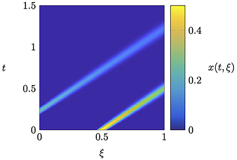
Figure 1. Linear advection–diffusion equation: pseudocolor plot of the FOM solution.

In the following, we proceed similarly as in [7] and approximate the FOM state by a linear combination of transformed modes using an extended domain shift operator as transformation operator [cf. [7], section 7.2 for the details]. On the space-discrete level, the shift operation requires an interpolation scheme for obtaining values of the underlying continuous function in between the spatial grid points. To this end, we employ cubic spline interpolation. The resulting approximation ansatz takes the form

$\begin{array}{ll}{x}_h(t)\approx {\displaystyle \sum _{i=1}^{r-1}}{\alpha }_i(t){\mathcal{T}}_{\text{ext}}(p(t)){\varphi }_i\text{ for all }t\in 𝕀,\hfill & (40)\end{array}$

where ${\mathcal{T}}_{\text{ext}}:ℝ\to {ℝ}^{n,d_{\varphi }}$ with n: = N+2 is the discretized analog of the extended domain shift operator, p:𝕀 → ℝ corresponds to the shift amount, ${\varphi }_1,\dots ,{\varphi }_{r-1}\in {ℝ}^{d_{\varphi }}$ are the modes, α₁, …, α_r−1:𝕀 → ℝ the corresponding amplitudes, and d_ϕ the number of spatial grid points of the extended domain. We note that (40) may be written as a separable ansatz of the form (3) by defining $V_{\text{s}}:ℝ\to {ℝ}^{n,r-1}$ via

$\begin{array}{l}{V}_{\text{s}}(p)≔T_{\text{ext}}(p)\left[\begin{array}{c}{\varphi }_1\cdots {\varphi }_{r-1}\hfill \end{array}\right].\hfill \end{array}$

Based on the snapshot data depicted in Figure 1, we determine r−1 = 3 modes via the residual minimization approach presented in [7, 96]. The resulting relative offline error is 0.71%. In comparison, the classical POD approach requires around 30 modes to achieve the same accuracy. Afterwards, we use the structure-preserving projection framework detailed in section 4 to obtain a corresponding port-Hamiltonian ROM of the form (5) with coefficients as in (31). The resulting online error is 1.2%. To demonstrate the energy consistency of the ROM, Figure 2 depicts the (discretized) time derivative of the ROM Hamiltonian $\tilde{\mathcal{H}}$ as well as the corresponding dissipation and supply rate at the midpoints of the discrete time intervals [cf. section 3.2]. Especially, we observe that the power balance (14) is approximately satisfied, as the graphs corresponding to $\frac{\text{d}\tilde{\mathcal{H}}}{\text{d}t}$ and $\tilde{\mathcal{S}}-\tilde{\mathcal{D}}$ lie on top of each other. The fact that the power balance is only approximately satisfied is illustrated in Table 1, where the corresponding mean and maximum errors are summarized for three different values of the time step size. Especially, the results indicate that the error is mainly due to the time discretization, as the errors decrease with decreasing time step size. We note that the implicit midpoint rule would yield a time-discrete system where the power balance is satisfied without any error, if the ROM Hamiltonian were a quadratic function of the ROM state [cf. [63, 97]]. However, due to the nonlinear approximation ansatz this is not the case here [cf. (6)].

FIGURE 2

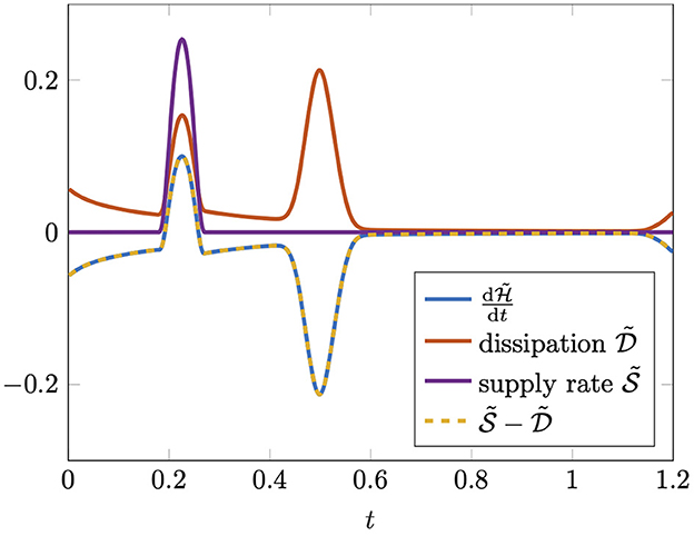
Figure 2. Linear advection–diffusion equation: comparison of the temporal change of the ROM Hamiltonian $\tilde{\mathcal{H}}$ and the corresponding dissipation $\tilde{\mathcal{D}}$ and supply rate $\tilde{\mathcal{S}}$.

TABLE 1

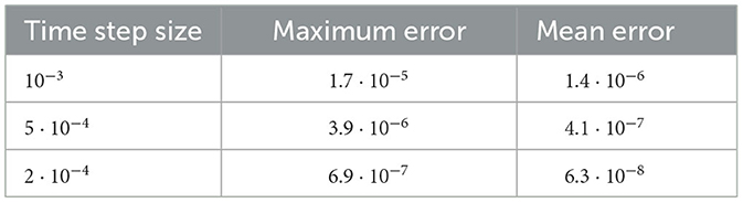
Table 1. Linear advection–diffusion equation: comparison of the maximum and mean errors in the ROM power balance for different time step sizes.

5.3. Wildland fire model

As second example, we consider a model which describes the dynamics of a wildland fire [cf. [61, 62]]. The governing equations on a one-dimensional spatial domain Ω = (a, b) are given by

$\begin{array}{ll}\begin{array}{c}{\partial }_{t}T=k{\partial }_{\xi \xi }T-w{\partial }_{\xi }T+\alpha (S\theta (T,\beta )-\gamma T),\hfill \\ {\partial }_{t}S=-\zeta S\theta (T,\beta ),\hfill \end{array}\hfill & (41)\end{array}$

where the unknowns are the relative temperature $T:𝕀\times \overline{\Omega }\to ℝ$ and the supply mass fraction $S:𝕀\times \overline{\Omega }\to ℝ$. Furthermore, the constants k, α, β, γ, ζ∈ℝ_>0 and w∈ℝ are assumed to be given and θ:ℝ × ℝ → ℝ is defined via

$\begin{array}{l}\theta (T,\beta )≔\{\begin{array}{cc}exp\left(-\frac{\beta }{T}\right),\hfill & \text{if }T>0,\hfill \\ 0,\hfill & \text{otherwise}.\hfill \end{array}\hfill \end{array}$

For the physical meaning of these coefficients, we refer to [61, 62]. Moreover, the system (41) is closed via appropriate initial conditions and periodic boundary conditions [cf. [61]].

In contrast to the previous section, we follow [61] for the spatial semi-discretization of (41) and perform a central finite difference scheme based on an equidistant grid with grid size $h=\frac{b-a}{N+1}$, N∈ℕ. The resulting finite-dimensional system reads

$\begin{array}{ll}\left[\begin{array}{c}{\dot{x}}_1(t)\\ {\dot{x}}_2(t)\end{array}\right]=\left[\begin{array}{cc}k{D}_2-w{D}_1-\alpha \gamma I_{N+1}& \alpha \Theta (x_1(t),\beta )\\ 0& -\zeta \Theta (x_1(t),\beta )\end{array}\right]\left[\begin{array}{c}{x}_1(t)\\ x_2(t)\end{array}\right],& (42)\end{array}$

where $x_1,x_2:𝕀\to {ℝ}^{N+1}$ correspond to approximations of T and S at the spatial grid points ih for i = 1, …, N+1. Moreover, $D_1=-D_1^{\top }$ and $D_2=D_2^{\top }\le 0$ are finite difference approximations of the first and second spatial derivative, respectively, and the function Θ:ℝ^N+1×ℝ → ℝ^{N+1, N+1} is given by

$\begin{array}{l}\Theta (x_1,\beta )≔\text{diag}(\theta ({\left[x_1\right]}_1,\beta ),\dots ,\theta ({\left[x_1\right]}_{N+1},\beta )).\end{array}$

In the following, we demonstrate that the semi-discretized wildland fire model (42) may be formulated as a dissipative Hamiltonian system. To this end, we introduce $\eta :=\frac{\alpha }{4\gamma \zeta }$ and observe that (42) may be written as

$\begin{array}{ll}\begin{array}{c}\left[\begin{array}{c}{\dot{x}}_1(t)\\ {\dot{x}}_2(t)\end{array}\right]={\displaystyle ({\displaystyle \underset{≕J_1}{{\displaystyle \underbrace{\left[\begin{array}{cc}-w{D}_1& 0\\ 0& 0\end{array}\right]}}}}+{\displaystyle \underset{≕J_2(x_1(t))}{{\displaystyle \underbrace{\frac{\alpha }{2\eta }\left[\begin{array}{cc}0& \Theta (x_1(t),\beta )\\ -\Theta (x_1(t),\beta )& 0\end{array}\right]}}}})}{\displaystyle \underset{≕Q}{{\displaystyle \underbrace{\left[\begin{array}{cc}{I}_{N+1}& 0\\ 0& \eta I_{N+1}\end{array}\right]}}}}\left[\begin{array}{c}{x}_1(t)\\ x_2(t)\end{array}\right]\\ -{\displaystyle ({\displaystyle \underset{≕R_1}{{\displaystyle \underbrace{k\left[\begin{array}{cc}-D_2& 0\\ 0& 0\end{array}\right]}}}}+{\displaystyle \underset{≕R_2(x_1(t))}{{\displaystyle \underbrace{\left[\begin{array}{cc}\alpha \gamma I_{N+1}& -\frac{\alpha }{2\eta }\Theta (x_1(t),\beta )\\ -\frac{\alpha }{2\eta }\Theta (x_1(t),\beta )& \frac{\zeta }{\eta }\Theta (x_1(t),\beta )\end{array}\right]}}}})}{\displaystyle \underset{=Q}{{\displaystyle \underbrace{\left[\begin{array}{cc}{I}_{N+1}& 0\\ 0& \eta I_{N+1}\end{array}\right]}}}}\left[\begin{array}{c}{x}_1(t)\\ x_2(t)\end{array}\right].\end{array}& (43)\end{array}$

Here, we note that Q is symmetric and positive definite since η is positive and that J₂ and R₂ are pointwise skew-symmetric and symmetric, respectively. Furthermore, since D₁ is skew-symmetric and D₂ is symmetric and negative semi-definite, we infer that J₁ is skew-symmetric and that R₁ is symmetric and positive semi-definite. Thus, if we can show that additionally R₂ is pointwise positive semi-definite, we may conclude that (43) is a dissipative Hamiltonian system. For this purpose, let z = [^p⊤q⊤]⊤∈ℝ^2(N+1) with p, q∈ℝ^N+1 and u∈ℝ^N+1 be arbitrary. Then, we obtain

$\begin{array}{l}{z}^{\top }{R}_2(u)z=\alpha \gamma p^{\top }p+\frac{1}{\eta }{\displaystyle \sum _{i=1}^{N+1}}(\zeta \theta (u_i,\beta )q_i^2-\alpha \theta (u_i,\beta )p_i{q}_i)\\ =\gamma {\displaystyle \sum _{i=1}^{N+1}}{\displaystyle \left({\displaystyle \underset{≕s_i}{{\displaystyle \underbrace{\alpha p_i^2-4\zeta \theta (u_i,\beta )p_i{q}_i+\frac{4{\zeta }^2}{\alpha }\theta (u_i,\beta )q_i^2}}}}\right)}.\end{array}$

In the case where u_i ≤ 0 holds for some i∈{1, …, N+1}, we have θ(u_i, β) = 0 and, hence, s_i≥0. Otherwise, we obtain

$\begin{array}{l}{s}_i=\alpha p_i^2-4\zeta exp\left(-\frac{\beta }{u_i}\right)p_i{q}_i+\frac{4{\zeta }^2}{\alpha }exp\left(-\frac{\beta }{u_i}\right)q_i^2\\ \ge \alpha p_i^2-4\zeta exp\left(-\frac{\beta }{u_i}\right)p_i{q}_i+\frac{4{\zeta }^2}{\alpha }exp\left(-\frac{2\beta }{u_i}\right)q_i^2\\ =\alpha p_i^2-4\zeta exp\left(-\frac{\beta }{u_i}\right)p_i{q}_i+\frac{4{\zeta }^2}{\alpha }{\left(exp\left(-\frac{\beta }{u_i}\right)\right)}^2{q}_i^2\\ ={\left(\sqrt{\alpha }{p}_i-\frac{2\zeta }{\sqrt{\alpha }}exp\left(-\frac{\beta }{u_i}\right)q_i\right)}^2\ge 0.\end{array}$

Consequently, R₂ is pointwise symmetric and positive semi-definite and, hence, (43) is a dissipative Hamiltonian formulation of (42) with J: = J₁+J₂ and R: = R₁+R₂.

For the following numerical experiments, we choose the physical and discretization parameters as detailed in [[61], section 5.4]. The resulting snapshots are depicted in Figure 3. Especially, we observe two traveling waves propagating through the computational domain.

FIGURE 3

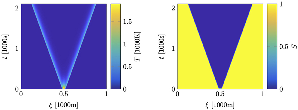
Figure 3. Wildland fire model: pseudocolor plot of the temperature (left) and supply mass fraction (right).

For the model reduction, we follow a different approach than in [61] since our main focus is on demonstrating the structure preservation rather than on the accuracy and evaluation time of the ROM. Similar to section 5.1, we approximate the FOM state by a linear combination of two transformed modes, one for each traveling wave. However, instead of an extended domain shift operator we use a periodic shift operator, which is again discretized using cubic spline interpolation. The corresponding approximation ansatz reads

$\begin{array}{ll}\left[\begin{array}{c}{x}_1(t)\\ x_2(t)\end{array}\right]\approx {\displaystyle \sum _{i=1}^2}{\alpha }_i(t)\left[\begin{array}{cc}{\mathcal{T}}_{\text{per}}(p_i(t))& 0\\ 0& {\mathcal{T}}_{\text{per}}(p_i(t))\end{array}\right]\left[\begin{array}{c}{\varphi }_{i,\text{T}}\\ {\varphi }_{i,\text{S}}\end{array}\right],& (44)\end{array}$

where ${\mathcal{T}}_{\text{per}}:ℝ\to {ℝ}^{n,n}$ with n: = N+1 is the discretized analog of the periodic shift operator and ϕ_{i, T} and ϕ_{i, S} denote the temperature and supply mass fraction block component of the ith mode, respectively, for i = 1, 2. Similarly as in section 5.1, this may be written as a separable ansatz of the form (3).

As in the previous subsection, the modes are determined via residual minimization yielding a relative offline error of 13%. As demonstrated in [61], the error may be significantly reduced by increasing the mode numbers and introducing a suitable time interval splitting. However, for illustrating the structure preservation, the relatively coarse approximation based on two shifted modes is sufficient here. In comparison, the classical POD approach requires 40 modes to achieve the same accuracy.

In the following, we compare two different ROMs which are both integrated in time using the implicit midpoint rule. The first one is based on the nonlinear Galerkin approach from [[7], section 5] and enforces the residual at t∈I to be orthogonal to the column space of $\left[V_{\text{s}}(p(t))\widehat{V_{\text{s}}}(p(t))\alpha (t)\right]$. On the other hand, the second ROM is based on the structure-preserving projection framework outlined in section 4, i.e., it enforces the residual at t∈𝕀 to be orthogonal to the column space of $Q\left[V_{\text{s}}(p(t))\widehat{V_{\text{s}}}(p(t))\alpha (t)\right]$ with Q as in (43). The corresponding online approximations of the temperature field are compared in Figure 4. The non-structure-preserving ROM based on the Galerkin approach yields a solution where the temperature rapidly decreases to zero and the fire goes out before traveling combustion waves may develop. On the other-hand, the approximation obtained by the structure-preserving ROM reveals traveling combustion waves, although the flame speeds are significantly smaller than the ones obtained by the corresponding FOM. Furthermore, Figure 5 illustrates that the unsatisfactory solution obtained by the non-structure-preserving ROM is accompanied by an energy inconsistency. Especially, at the beginning of the time interval, the decline of the Hamiltonian is much greater than the corresponding dissipation, i.e., the power balance is clearly violated. Since the ROM Hamiltonian is a squared function of the amplitudes α [cf. (6)], this rapid decline is also reflected in the abrupt temperature decrease observed in Figure 4. On the other hand, the structure-preserving MOR approach yields an energy-consistent ROM as illustrated in Figure 5, right.

FIGURE 4

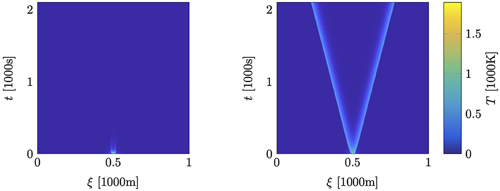
Figure 4. Wildland fire model: pseudocolor plots of the temperature approximations using the non-structure-preserving ROM (left) and the structure-preserving one (right).

FIGURE 5

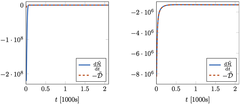
Figure 5. Wildland fire model: comparison of the temporal change of the ROM Hamiltonian $\tilde{\mathcal{H}}$ and the corresponding negative dissipation $-\tilde{\mathcal{D}}$ using the non-structure-preserving ROM (left) and the structure-preserving one (right).

The results addressed in the previous paragraph demonstrate that the structure-preserving MOR approach does not only ensure port-Hamiltonian ROMs, but it may sometimes also lead to a gain in accuracy. However, at this point we emphasize that there is in general no guarantee that this is the case and in most of our numerical experiments the accuracies of the structure-preserving and the non-structure-preserving ROMs have been comparable. The theory from section 4 only ensures the energy consistency of the ROM, but it does not include any statements about the accuracy in comparison to the FOM.

6. Conclusion

In this paper, we introduce a structure-preserving model order reduction (MOR) framework for port-Hamiltonian (pH) systems based on a special class of nonlinear approximation ansatzes. In particular, we consider so-called separable ansatzes, which are linear with respect to a part of the reduced-order model (ROM) state. Such ansatzes are for instance relevant in the context of transport-dominated systems which are challenging for classical methods based on linear subspace approximations. Based on the considered class of ansatzes, we demonstrate how to obtain a port-Hamiltonian ROM via projection, provided that the corresponding full-order model (FOM) has a certain pH structure, which includes linear as well as a wide range of nonlinear pH systems. Moreover, in a special case, we obtain ROMs which are not only pH, but also optimal in the sense that the derivative of the ROM state minimizes a certain weighted norm of the residual. In addition, we provide sufficient conditions which ensure that the resulting approximation of the FOM state is bounded. Finally, the theoretical findings are illustrated by means of a linear advection–diffusion problem with non-periodic boundary conditions and a nonlinear reaction–diffusion system modeling the spread of wildland fires.

While we have only considered a special class of nonlinear approximation ansatzes, an interesting future research direction is to derive structure-preserving MOR schemes based on more general nonlinear ansatzes. This would especially allow to obtain port-Hamiltonian ROMs via projection onto nonlinear manifolds which are parametrized by artificial neural networks. Another question not addressed in this manuscript is the preservation of algebraic constraints in cases where the FOM is given by a pH system of differential–algebraic equations. While corresponding approaches already exist in the context of classical MOR based on linear ansatzes as mentioned in Remark 2.1, this is still an open problem in the context of nonlinear ansatzes.

Data availability statement

The original contributions presented in the study are included in the article/supplementary material, further inquiries can be directed to the corresponding author.

Author contributions

The author confirms being the sole contributor of this work and has approved it for publication.

Funding

This work was supported by the Deutsche Forschungsgemeinschaft (DFG, German Research Foundation) Collaborative Research Center Transregio 96 Thermo-energetic design of machine tools—A systemic approach to solve the conflict between power efficiency, accuracy and productivity demonstrated at the example of machining production, project number 174223256. The publication of this article was funded by Chemnitz University of Technology and by the Deutsche Forschungsgemeinschaft—491193532.

Acknowledgments

I would like to thank Volker Mehrmann and Riccardo Morandin from TU Berlin for helpful discussions.

Conflict of interest

The author declares that the research was conducted in the absence of any commercial or financial relationships that could be construed as a potential conflict of interest.

Publisher's note

All claims expressed in this article are solely those of the authors and do not necessarily represent those of their affiliated organizations, or those of the publisher, the editors and the reviewers. Any product that may be evaluated in this article, or claim that may be made by its manufacturer, is not guaranteed or endorsed by the publisher.

References

1. Antoulas AC. Approximation of Large-Scale Dynamical Systems. Philadelphia, PA: Society for Industrial and Applied Mathematics (2005). doi: 10.1137/1.9780898718713

CrossRef Full Text | Google Scholar

2. Benner P, Ohlberger M, Cohen A, Willcox K. Model Reduction and Approximation. Philadelphia, PA: Society for Industrial and Applied Mathematics (2017). doi: 10.1137/1.9781611974829

CrossRef Full Text | Google Scholar

3. Hesthaven JS, Rozza G, Stamm B. Certified Reduced Basis Methods for Parametrized Partial Differential Equations. Cham: Springer International Publishing (2016). doi: 10.1007/978-3-319-22470-1

CrossRef Full Text | Google Scholar

4. Quarteroni A, Manzoni A, Negri F. Reduced Basis Methods for Partial Differential Equations. Cham: Springer International Publishing (2016). doi: 10.1007/978-3-319-15431-2

CrossRef Full Text | Google Scholar

5. Schilders WHA, van der Vorst HA, Rommes J. Model Order Reduction: Theory, Research Aspects and Applications. Berlin: Springer Berlin Heidelberg (2008). doi: 10.1007/978-3-540-78841-6

CrossRef Full Text | Google Scholar

6. Barnett J, Farhat C. Quadratic approximation manifold for mitigating the Kolmogorov barrier in nonlinear projection-based model order reduction. J Comput Phys. (2022) 464:111348. doi: 10.1016/j.jcp.2022.111348

CrossRef Full Text | Google Scholar

7. Black F, Schulze P, Unger B. Projection-based model reduction with dynamically transformed modes. ESAIM Math Model Numer Anal. (2020) 54:2011–43. doi: 10.1051/m2an/2020046

CrossRef Full Text | Google Scholar

8. Cagniart N, Maday Y, Stamm B. Model order reduction for problems with large convection effects. In:Chetverushkin BN, Fitzgibbon W, Kuznetsov YA, Neittaanmäki P, Periaux J, Pironneau O, , editors. Contributions to Partial Differential Equations and Applications. Cham: Springer International Publishing (2019). p. 131–50. doi: 10.1007/978-3-319-78325-3_10

CrossRef Full Text | Google Scholar

9. Fresca S, Dedé L, Manzoni A. A comprehensive deep learning-based approach to reduced order modeling of nonlinear time-dependent parametrized PDEs. J Sci Comput. (2021) 87:61. doi: 10.1007/s10915-021-01462-7

CrossRef Full Text | Google Scholar

10. Kim Y, Choi Y, Widemann D, Zohdi T. A fast and accurate physics-informed neural network reduced order model with shallow masked autoencoder. J Comput Phys. (2022) 451:110841. doi: 10.1016/j.jcp.2021.110841

CrossRef Full Text | Google Scholar

11. Lee K, Carlberg KT. Model reduction of dynamical systems on nonlinear manifolds using deep convolutional autoencoders. J Comput Phys. (2019) 404:108973. doi: 10.1016/j.jcp.2019.108973

PubMed Abstract | CrossRef Full Text | Google Scholar

12. Ohlberger M, Rave S. Reduced basis methods: success, limitations and future challenges. In: Proceedings of the Conference Algoritmy. Vysoké Tatry (2016).

Google Scholar

13. Antoulas AC. A new result on passivity preserving model reduction. Syst Control Lett. (2005) 54:361–74. doi: 10.1016/j.sysconle.2004.07.007

CrossRef Full Text | Google Scholar

14. Benner P, Stykel T. Model order reduction for differential-algebraic equations: a survey. In:Ilchmann A, Reis T, , editors. Surveys in Differential-Algebraic Equations IV. Cham: Springer International Publishing (2017). p. 107–60. doi: 10.1007/978-3-319-46618-7_3

CrossRef Full Text | Google Scholar

15. Breiten T, Unger B. Passivity preserving model reduction via spectral factorization. Automatica. (2022) 142:110368. doi: 10.1016/j.automatica.2022.110368

CrossRef Full Text | Google Scholar

16. Castañé Selga R, Lohmann B, Eid R. Stability preservation in projection-based model order reduction of large scale systems. Eur J Control. (2012) 18:122–32. doi: 10.3166/ejc.18.122-132

CrossRef Full Text | Google Scholar

17. Cheng X, Scherpen JMA. Model reduction methods for complex network systems. Annu Rev Control Robot Auton Syst. (2021) 4:425–53. doi: 10.1146/annurev-control-061820-083817

CrossRef Full Text | Google Scholar

18. Monshizadeh N, Trentelman HL, Camlibel MK. Stability and synchronization preserving model reduction of multi-agent systems. Syst Control Lett. (2013) 62:1–10. doi: 10.1016/j.sysconle.2012.10.011

CrossRef Full Text | Google Scholar

19. Pulch R. Stability-preserving model order reduction for linear stochastic Galerkin systems. J Math Ind. (2019) 9:10. doi: 10.1186/s13362-019-0067-6

CrossRef Full Text | Google Scholar

20. Sorensen DC. Passivity preserving model reduction via interpolation of spectral zeros. Syst Control Lett. (2005) 54:347–60. doi: 10.1016/j.sysconle.2004.07.006

CrossRef Full Text | Google Scholar

21. Kotyczka P. Numerical Methods for Distributed Parameter Port-Hamiltonian Systems. Munich: TUM University Press (2019).

Google Scholar

22. Mehrmann V, Unger B. Control of port-Hamiltonian differential-algebraic systems and applications. Acta Numer. (2023) 32:395–515. doi: 10.1017/S0962492922000083

CrossRef Full Text | Google Scholar

23. van der Schaft AJ, Jeltsema D. Port-Hamiltonian systems theory: an introductory overview. Found Trends Syst Control. (2014) 1:173–378. doi: 10.1561/2600000002

CrossRef Full Text | Google Scholar

24. Duindam V, Macchelli A, Stramigioli S, Bruyninckx H. Modeling and Control of Complex Physical Systems. Berlin; Heidelberg: Springer-Verlag (2009). doi: 10.1007/978-3-642-03196-0

CrossRef Full Text | Google Scholar

25. Ortega R, van der Schaft A, Castaños F, Astolfi A. Control by interconnection and standard passivity-based control of port-Hamiltonian systems. IEEE Trans Automat Control. (2008) 53:2527–42. doi: 10.1109/TAC.2008.2006930

CrossRef Full Text | Google Scholar

26. van der Schaft A. Port-Hamiltonian modeling for control. Annu Rev Control Robot Auton Syst. (2020) 3:393–416. doi: 10.1146/annurev-control-081219-092250

CrossRef Full Text | Google Scholar

27. Schaller M, Philipp F, Faulwasser T, Worthmann K, Maschke B. Control of port-Hamiltonian systems with minimal energy supply. Eur J Control. (2021) 62:33–40. doi: 10.1016/j.ejcon.2021.06.017

CrossRef Full Text | Google Scholar

28. Altmann R, Mehrmann V, Unger B. Port-Hamiltonian formulations of poroelastic network models. Math Comput Model Dyn Syst. (2021) 27:429–52. doi: 10.1080/13873954.2021.1975137

CrossRef Full Text | Google Scholar

29. Fiaz S, Zonetti D, Ortega R, Scherpen JMA, van der Schaft AJ. A port-Hamiltonian approach to power network modeling and analysis. Eur J Control. (2013) 19:477–85. doi: 10.1016/j.ejcon.2013.09.002

PubMed Abstract | CrossRef Full Text | Google Scholar

30. Altmann R, Schulze P. A port-Hamiltonian formulation of the Navier-Stokes equations for reactive flows. Syst Control Lett. (2017) 100:51–5. doi: 10.1016/j.sysconle.2016.12.005

CrossRef Full Text | Google Scholar

31. Bansal H, Schulze P, Abbasi MH, Zwart H, Iapichino L, Schilders WHA, et al. Port-Hamiltonian formulation of two-phase flow models. Syst Control Lett. (2021) 149:104881. doi: 10.1016/j.sysconle.2021.104881

CrossRef Full Text | Google Scholar

32. Brugnoli A, Alazard D, Pommier-Budinger V, Matignon D. Port-Hamiltonian formulation and symplectic discretization of plate models part I: mindlin model for thick plates. Appl Math Model. (2019) 75:940–60. doi: 10.1016/j.apm.2019.04.035

CrossRef Full Text | Google Scholar

33. Brugnoli A, Alazard D, Pommier-Budinger V, Matignon D. Port-Hamiltonian formulation and symplectic discretization of plate models part II: Kirchhoff model for thin plates. Appl Math Model. (2019) 75:961–81. doi: 10.1016/j.apm.2019.04.036

CrossRef Full Text | Google Scholar

34. Gernandt H, Haller FE, Reis T, van der Schaft AJ. Port-Hamiltonian formulation of nonlinear electrical circuits. J Geom Phys. (2021) 159:103959. doi: 10.1016/j.geomphys.2020.103959

CrossRef Full Text | Google Scholar

35. Hoang H, Couenne F, Jallut C, Le Gorrec Y. The port Hamiltonian approach to modeling and control of Continuous Stirred Tank Reactors. J Process Control. (2011) 21:1449–58. doi: 10.1016/j.jprocont.2011.06.014

CrossRef Full Text | Google Scholar

36. Macchelli A, Melchiorri C. Modeling and control of the Timoshenko beam. The distributed port Hamiltonian approach. SIAM J Control Optim. (2004) 43:743–67. doi: 10.1137/S0363012903429530

CrossRef Full Text | Google Scholar

37. Mora LA, Le Gorrec Y, Matignon D, Ramirez H, Yuz JI. On port-Hamiltonian formulations of 3-dimensional compressible Newtonian fluids. Phys Fluids. (2021) 33:117117. doi: 10.1063/5.0067784

CrossRef Full Text | Google Scholar

38. Ramirez H, Maschke B, Sbarbaro D. Irreversible port-Hamiltonian systems: a general formulation of irreversible processes with application to the CSTR. Chem Eng Sci. (2013) 89:223–34. doi: 10.1016/j.ces.2012.12.002

CrossRef Full Text | Google Scholar

39. Rashad R, Califano F, Schuller FP, Stramigioli S. Port-Hamiltonian modeling of ideal fluid flow: part I. Foundations and kinetic energy. J Geom Phys. (2021) 164:104201. doi: 10.1016/j.geomphys.2021.104201

CrossRef Full Text | Google Scholar

40. Wang L, Maschke B, van der Schaft A. Port-Hamiltonian modeling of non-isothermal chemical reaction networks. J Math Chem. (2018) 56:1707–27. doi: 10.1007/s10910-018-0882-9

CrossRef Full Text | Google Scholar

41. Warsewa A, Böhm M, Sawodny O, Tarín C. A port-Hamiltonian approach to modeling the structural dynamics of complex systems. Appl Math Model. (2021) 89:1528–46. doi: 10.1016/j.apm.2020.07.038

CrossRef Full Text | Google Scholar

42. Cardoso-Ribeiro FL, Matignon D, Pommier-Budinger V. A port-Hamiltonian model of liquid sloshing in moving containers and application to a fluid-structure system. J Fluids Struct. (2017) 69:402–27. doi: 10.1016/j.jfluidstructs.2016.12.007

CrossRef Full Text | Google Scholar

43. Falaize A, Hélie T. Passive simulation of the nonlinear port-Hamiltonian modeling of a Rhodes piano. J Sound Vib. (2017) 390:289–309. doi: 10.1016/j.jsv.2016.11.008

CrossRef Full Text | Google Scholar

44. Voß T, Scherpen JMA. Port-Hamiltonian modeling of a nonlinear Timoshenko beam with piezo actuation. SIAM J Control Optim. (2014) 52:493–519. doi: 10.1137/090774598

CrossRef Full Text | Google Scholar

45. Vu NMT, Lefèvre L, Maschke B. A structured control model for the thermo-magneto-hydrodynamics of plasmas in tokamaks. Math Comput Model Dyn Syst. (2016) 22:181–206. doi: 10.1080/13873954.2016.1154874

CrossRef Full Text | Google Scholar

46. Zhou W, Wu Y, Hu H, Li Y, Wang Y. Port-Hamiltonian modeling and IDA-PBC control of an IPMC-actuated flexible beam. Actuators. (2021) 10:236. doi: 10.3390/act10090236

CrossRef Full Text | Google Scholar

47. Borja P, Scherpen JMA, Fujimoto K. Extended balancing of continuous LTI systems: a structure-preserving approach. IEEE Trans Automat Control. (2021) 68:257–71. doi: 10.1109/TAC.2021.3138645

CrossRef Full Text | Google Scholar

48. Breiten T, Morandin R, Schulze P. Error bounds for port-Hamiltonian model and controller reduction based on system balancing. Comput Math with Appl. (2022) 116:100–15. doi: 10.1016/j.camwa.2021.07.022

CrossRef Full Text | Google Scholar

49. Hartmann C, Vulcanov VM, Schütte C. Balanced truncation of linear second-order systems: a Hamiltonian approach. Multiscale Model Simul. (2010) 8:1348–67. doi: 10.1137/080732717

CrossRef Full Text | Google Scholar

50. Polyuga RV, van der Schaft AJ. Effort- and flow-constraint reduction methods for structure preserving model reduction of port-Hamiltonian systems. Syst Control Lett. (2012) 61:412–21. doi: 10.1016/j.sysconle.2011.12.008

CrossRef Full Text | Google Scholar

51. Egger H, Kugler T, Liljegren-Sailer B, Marheineke N, Mehrmann V. On structure-preserving model reduction for damped wave propagation in transport networks. SIAM J Sci Comput. (2018) 40:A331–65. doi: 10.1137/17M1125303

CrossRef Full Text | Google Scholar

52. Giftthaler M, Wolf T, Panzer HKF, Lohmann B. Parametric model order reduction of port-Hamiltonian systems by matrix interpolation. Automatisierungstechnik. (2014) 62:619–28. doi: 10.1515/auto-2013-1072

CrossRef Full Text | Google Scholar

53. Gugercin S, Polyuga RV, Beattie C, van der Schaft A. Structure-preserving tangential interpolation for model reduction of port-Hamiltonian systems. Automatica. (2012) 48:1963–74. doi: 10.1016/j.automatica.2012.05.052

CrossRef Full Text | Google Scholar

54. Ionescu TC, Astolfi A. Families of moment matching based, structure preserving approximations for linear port Hamiltonian systems. Automatica. (2013) 49:2424–34. doi: 10.1016/j.automatica.2013.05.006

CrossRef Full Text | Google Scholar

55. Wolf T, Lohmann B, Eid R, Kotyczka P. Passivity and structure preserving order reduction of linear port-Hamiltonian systems using Krylov subspaces. Eur J Control. (2010) 16:401–6. doi: 10.3166/ejc.16.401-406

CrossRef Full Text | Google Scholar

56. Sato K. Riemannian optimal model reduction of linear port-Hamiltonian systems. Automatica. (2018) 93:428–34. doi: 10.1016/j.automatica.2018.03.051

CrossRef Full Text | Google Scholar

57. Schwerdtner P, Voigt M. Adaptive sampling for structure-preserving model order reduction of port-Hamiltonian systems. IFAC-PapersOnLine. (2021) 54:143–8. doi: 10.1016/j.ifacol.2021.11.069

CrossRef Full Text | Google Scholar

58. Chaturantabut S, Beattie C, Gugercin S. Structure-preserving model reduction for nonlinear port-Hamiltonian systems. SIAM J Sci Comput. (2016) 38:B837–65. doi: 10.1137/15M1055085

CrossRef Full Text | Google Scholar

59. Gugercin S, Antoulas AC, Beattie C. H₂ model reduction for large-scale linear dynamical systems. SIAM J Matrix Anal Appl. (2008) 30:609–38. doi: 10.1137/060666123

CrossRef Full Text | Google Scholar

60. Chaturantabut S, Sorensen DC. Nonlinear model reduction via discrete empirical interpolation. SIAM J Sci Comput. (2010) 32:2737–64. doi: 10.1137/090766498

CrossRef Full Text | Google Scholar

61. Black F, Schulze P, Unger B. Efficient wildland fire simulation via nonlinear model order reduction. Fluids. (2021) 6:280. doi: 10.3390/fluids6080280

CrossRef Full Text | Google Scholar

62. Mandel J, Bennethum LS, Beezley JD, Coen JL, Douglas CC, Kim M, et al. A wildland fire model with data assimilation. Math Comput Simul. (2008) 79:584–606. doi: 10.1016/j.matcom.2008.03.015

CrossRef Full Text | Google Scholar

63. Mehrmann V, Morandin R. Structure-preserving discretization for port-Hamiltonian descriptor systems. In: Proceedings of the 58th IEEE Conference on Decision and Control. Nice (2019). p. 6863–8. doi: 10.1109/CDC40024.2019.9030180

CrossRef Full Text | Google Scholar

64. Beattie C, Gugercin S, Mehrmann V. Structure-preserving interpolatory model reduction for port-Hamiltonian differential-algebraic systems. In:Beattie C, Benner P, Embree M, Gugercin S, Lefteriu S, , editors. Realization and Model Reduction of Dynamical Systems: A Festschrift in Honor of the 70th Birthday of Thanos Antoulas. Cham: Springer Nature Switzerland (2022). p. 235–54. doi: 10.1007/978-3-030-95157-3_13

CrossRef Full Text | Google Scholar

65. Hauschild SA, Marheineke N, Mehrmann V. Model reduction techniques for linear constant coefficient port-Hamiltonian differential-algebraic systems. Control Cybern. (2019) 48:125–52. doi: 10.1002/pamm.201900040

CrossRef Full Text | Google Scholar

66. Kunkel P, Mehrmann VL. Differential-Algebraic Equations-Analysis and Numerical Solution. Zürich: EMS Publishing House (2006). doi: 10.4171/017

CrossRef Full Text | Google Scholar

67. Khalil HK. Nonlinear Systems. 3rd Edn. Upper Saddle River, NJ: Prentice Hall (2002).

Google Scholar

68. Rashad R, Califano F, van der Schaft AJ, Stramigioli S. Twenty years of distributed port-Hamiltonian systems: a literature review. IMA J Math Control Inf . (2020) 37:1400–22. doi: 10.1093/imamci/dnaa018

CrossRef Full Text | Google Scholar

69. van der Schaft A. L₂-Gain and Passivity Techniques in Nonlinear Control, 3rd Edn. Cham: Springer International Publishing (2017). doi: 10.1007/978-3-319-49992-5

CrossRef Full Text | Google Scholar

70. Byrnes CI, Isidori A, Willems JC. Passivity, feedback equivalence, and the global stabilization of minimum phase nonlinear systems. IEEE Trans Automat Control. (1991) 36:1228–40. doi: 10.1109/9.100932

CrossRef Full Text | Google Scholar

71. Vidyasagar M. Nonlinear Systems Analysis, 2nd Edn. Englewood Cliffs, NJ: Prentice-Hall (1993).

Google Scholar

72. Carlberg K, Barone M, Antil H. Galerkin v. least-squares Petrov-Galerkin projection in nonlinear model reduction. J Comput Phys. (2017) 330:693–734. doi: 10.1016/j.jcp.2016.10.033

CrossRef Full Text | Google Scholar

73. Bernstein DS. Matrix Mathematics: Theory, Facts, and Formulas, 2nd Edn. Princeton, NJ: Princeton University Press (2009). doi: 10.1515/9781400833344

PubMed Abstract | CrossRef Full Text | Google Scholar

74. Benner P, Breiten T. Model order reduction based on system balancing. In:Benner P, Ohlberger M, Cohen A, Willcox K, , editors. Model Reduction and Approximation. Philadelphia, PA: Society for Industrial and Applied Mathematics (2017). p. 261–95. doi: 10.1137/1.9781611974829.ch6

CrossRef Full Text | Google Scholar

75. Moore BC. Principal component analysis in linear systems: controllability, observability, and model reduction. IEEE Trans Automat Control. (1981) 26:17–32. doi: 10.1109/TAC.1981.1102568

PubMed Abstract | CrossRef Full Text | Google Scholar

76. Antoulas AC, Beattie CA, Güğercin S. Interpolatory Methods for Model Reduction. Philadelphia, PA: Society for Industrial and Applied Mathematics (2020). doi: 10.1137/1.9781611976083

CrossRef Full Text | Google Scholar

77. Benner P, Feng L. Model order reduction based on moment-matching. In:Benner P, Grivet-Talocia S, Quarteroni A, Rozza G, Schilders W, Miguel Silveira L, , editors. Model Order Reduction-Volume 1: System- and Data-Driven Methods and Algorithms. Berlin: De Gruyter (2021). p. 57–96. doi: 10.1515/9783110498967-003

PubMed Abstract | CrossRef Full Text | Google Scholar

78. Berkooz G, Holmes P, Lumley JL. The proper orthogonal decomposition in the analysis of turbulent flows. Annu Rev Fluid Mech. (1993) 25:539–75. doi: 10.1146/annurev.fl.25.010193.002543

CrossRef Full Text | Google Scholar

79. Gubisch M, Volkwein S. Proper orthogonal decomposition for linear-quadratic optimal control. In:Benner P, Ohlberger M, Cohen A, Willcox K, , editors. Model Reduction and Approximation. Philadelphia, PA: Society for Industrial and Applied Mathematics (2017). p. 3–63. doi: 10.1137/1.9781611974829.ch1

CrossRef Full Text | Google Scholar

80. Gu C, Roychowdhury J. Model reduction via projection onto nonlinear manifolds, with applications to analog circuits and biochemical systems. In: IEEE/ACM International Conference on Computer Aided Design (ICCAD). San Jose (2008). p. 85–92.

Google Scholar

81. Kramer B, Willcox KE. Nonlinear model order reduction via lifting transformations and proper orthogonal decomposition. AIAA J. (2019) 57:2297–307. doi: 10.2514/1.J057791

CrossRef Full Text | Google Scholar

82. Alla A, Kutz JN. Nonlinear model order reduction via dynamic mode decomposition. SIAM J Sci Comput. (2017) 39:B778–96. doi: 10.1137/16M1059308

CrossRef Full Text | Google Scholar

83. Astrid P, Weiland S, Willcox K, Backx T. Missing point estimation in models described by proper orthogonal decomposition. IEEE Trans Automat Control. (2008) 53:2237–51. doi: 10.1109/TAC.2008.2006102

CrossRef Full Text | Google Scholar

84. Barrault M, Maday Y, Nguyen NC, Patera AT. An ‘empirical interpolation' method: application to efficient reduced-basis discretization of partial differential equations. C R Math Acad Sci Paris. (2004) 339:667–72. doi: 10.1016/j.crma.2004.08.006

CrossRef Full Text | Google Scholar

85. Carlberg K, Bou-Mosleh C, Farhat C. Efficient non-linear model reduction via a least-squares Petrov-Galerkin projection and compressive tensor approximations. Int J Numer Methods Eng. (2011) 86:155–81. doi: 10.1002/nme.3050

CrossRef Full Text | Google Scholar

86. Farhat C, Avery P, Chapman T, Cortial J. Dimensional reduction of nonlinear finite element dynamic models with finite rotations and energy-based mesh sampling and weighting for computational efficiency. Int J Numer Methods Eng. (2014) 98:625–62. doi: 10.1002/nme.4668

CrossRef Full Text | Google Scholar

87. Schulze P. Structure-preserving model reduction for port-Hamiltonian systems based on a special class of nonlinear approximation ansatzes. arXiv [preprint]: 2302.06479 (2023).

Google Scholar

88. Golub G, Pereyra V. Separable nonlinear least squares: the variable projection method and its applications. Inverse Probl. (2003) 19:R1–26. doi: 10.1088/0266-5611/19/2/201

PubMed Abstract | CrossRef Full Text | Google Scholar

89. Anderson W, Farazmand M. Evolution of nonlinear reduced-order solutions for PDEs with conserved quantities. SIAM J Sci Comput. (2022) 44:A176–97. doi: 10.1137/21M1415972

CrossRef Full Text | Google Scholar

90. Anderson W, Farazmand M. Shape-morphing reduced-order models for nonlinear Schrödinger equations. Nonlinear Dyn. (2022) 108:2889–902. doi: 10.1007/s11071-022-07448-w

CrossRef Full Text | Google Scholar

91. Rim D, Peherstorfer B, Mandli KT. Manifold approximations via transported subspaces: model reduction for transport-dominated problems. SIAM J Sci Comput. (2023) 45:A170–99. doi: 10.1137/20M1316998

CrossRef Full Text | Google Scholar

92. Rowley CW, Marsden JE. Reconstruction equations and the Karhunen-Loève expansion for systems with symmetry. Phys D. (2000) 142:1–19. doi: 10.1016/S0167-2789(00)00042-7

CrossRef Full Text | Google Scholar

93. Glavaski S, Marsden JE, Murray RM. Model reduction, centering, and the Karhunen-Loeve expansion. In: Proceedings of the 37th IEEE Conference on Decision and Control. Tampa, FL (1998). p. 2071–6.

Google Scholar

94. Agud Albesa L, Boix García M, Pla Ferrando ML, Cardona Navarrete SC. A study about the solution of convection-diffusion-reaction equation with Danckwerts boundary conditions by analytical, method of lines and Crank-Nicholson techniques. Math Methods Appl Sci. (2022) 46:2133–64. doi: 10.1002/mma.8633

CrossRef Full Text | Google Scholar

95. Danckwerts PV. Continuous flow systems: distribution of residence times. Chem Eng Sci. (1953) 2:1–13. doi: 10.1016/0009-2509(53)80001-1

CrossRef Full Text | Google Scholar

96. Schulze P, Reiss J, Mehrmann V. Model reduction for a pulsed detonation combuster via shifted proper orthogonal decomposition. In:King R, , editor. Active Flow and Combustion Control 2018. Cham: Springer International Publishing (2019). p. 271–86. doi: 10.1007/978-3-319-98177-2_17

CrossRef Full Text | Google Scholar

97. Kotyczka P, Lefèvre L. Discrete-time port-Hamiltonian systems: a definition based on symplectic integration. Syst Control Lett. (2019) 133:104530. doi: 10.1016/j.sysconle.2019.104530

CrossRef Full Text | Google Scholar