Mathematical modeling for the control of fly-borne mastitis disease in cattle

1. Introduction

The word mastitis is derived from two Greek words: masto (meaning mammary gland) and itis (meaning inflammation) [1]. Thus, mastitis is referred to as the inflammation of the mammary gland. Mastitis disease is caused by bacterial infection, trauma, or injury to the udder. It is the most common and expensive disease that affects dairy cattle throughout the world. Mastitis is caused by several different bacteria or other microorganisms (fungi, yeasts, and possibly viruses) that invade the udder, multiply and produce harmful substances there and then result in inflammation [2]. The most common microorganisms, causing mastitis, can be divided into two groups: (i) contagious bacteria (e.g., Staphylococcus aureus, Mycoplasma spp., and Streptococcus agalactiae) and (ii) environmental bacteria (e.g., Streptococcus uberis, Streptococcus dysgalactiae subsp. dysgalactiae, coliforms including Escherichia coli and Klebsiella spp.) [3].

Mastitis disease has well-recognized detrimental effects on animals' wellbeing and dairy farm profitability [4]. Mastitis can, directly, affect the mammary gland of the cow, leading to a significant reduction of the quantity and quality of the milk and, therefore, to reduced value of the production [5]. Despite decades of implementation of control strategies, mastitis continues to be one of the most significant and economically challenging problems of dairy cows [6, 7]. It reduces the productivity of the cows and the quality of milk causing enormous losses for breeders and, consequently, to the national income of the country [2]. According to the estimation of the National Mastitis Council (USA), mastitis costs more than $2 billion to dairy farmers annually [3, 7].

Mastitis is transmitted by direct contact between an infected and a susceptible animal which becomes infected by inhaling droplets disseminated in the environment. It can also be transmitted through an infected vector (such as a horn fly and, possibly, a housefly) [8–10]. The presentation of mastitis in a cow can be either a clinical or subclinical infection. In the subclinical type, the infection is asymptomatic and there are no visible changes in the appearance of the milk and/or the udder, milk production decreases by 10–20% with undesirable effect on its constituents and nutritional value rendering it of low quality and unfit for processing [11]. Subclinical (or acute) mastitis is the most common and economically harmful infection. Clinical mastitis, on the other hand, is characterized by heat, pain, swelling, and redness of the udder, along with reduced and an abnormal nature of milk yield. It is usually accompanied by a mild fever and animal depression. The affected quarter is sensitive to touch and painful to the animal. If acute mastitis is not attended, the inflammatory process persists for long, it gets converted into chronic mastitis which renders the milk-secreting tissue unable to produce any more milk. These changes are generally incurable and permanent [2]. The control of subclinical mastitis is more important than simply treating clinical cases because of the following reasons: The cows that have subclinical mastitis are reservoirs of organisms that lead to infection of other cows; and most clinical cases start as subclinical; thus, controlling subclinical mastitis is the best way to reduce the clinical cases [5]. Therefore, routine physical examination of the udder and diagnostic screening tests for early detection of mastitis and proper treatment of affected animals are of paramount importance to minimize losses due to subclinical and clinical mastitis [2].

Cows suffering from mastitis may recover spontaneously, but usually, drug therapy is required to maintain productivity [2]. Treatment of mastitis disease is achieved via systemic and intramammary administration of antibiotics, supportive fluid, and anti-inflammatory therapy [4]. Strict hygiene has to be maintained in cattle bedding to prevent transmission of infection during milking via contaminated milk, hands of the milker, and udder cloths (in the case of the milking machine) [2]. Culling of cows suffering from recurrent clinical mastitis (i.e., chronic mastitis) [2], and vector control via the application of insecticides (such as methoprene, synthetic pyrethroids, organophosphates, and abamectins) [9] are also good mastitis disease control measures.

Some mathematical studies have been conducted that focused on mastitis transmission from one udder-quarter to another in an infected cow [8, 12–14], even though clinical studies established the cow–cow and flies–cow transmissions [4, 5, 7, 10]. Therefore, the present study proposed an epidemic mathematical model for the control of mastitis disease in cattle in the presence of flies as vectors. The goals were to analyze the dynamic transmission and to investigate the impacts of various control measures available for vector-borne mastitis. The rest of this study is presented with the following organization: Section 2 provided the detail of the model's description and a domain in which it is feasible epidemiologically and well-posed mathematically. Section 3 demonstrated the analyses of the equilibrium points, which include the fundamental reproduction number derivation and analyses of local and global stabilities of the equilibrium points and the sensitivity analysis. Section 4 contained the model's numerical simulations and graphical illustrations and a discussion of the results. Section 5 included the conclusion of the study.

2. Mathematical model

To study the control of fly-borne mastitis disease in cattle using a mathematical model, a mathematical model is hereby formulated using a system of ordinary differential equations as follows. Furthermore, the model was shown to be well-posed by establishing the positivity of solutions and the region where the model is epidemiologically feasible.

2.1. Model formulation

The cattle population and fly population are the interacting host and vector populations, respectively. The cattle population is subdivided into the subpopulations of susceptible [S_c(t)], exposed [E(t)], subclinical infective [A(t)], clinical infective [I_c(t)], chronic infective [C(t)], and recovered cattle [R(t)], so that the total cattle population at any time, t, is given as:

$\begin{array}{ll}{N}_c\left(t\right)=S_c\left(t\right)+E\left(t\right)+A\left(t\right)+I_c\left(t\right)+C\left(t\right)+R\left(t\right).& (1)\end{array}$

The vector (flies) population is subdivided into the subpopulations of susceptible [S_v(t)] and infected flies [I_v(t)], and so that the total vector population at any time, t, is given as:

$\begin{array}{ll}{N}_v\left(t\right)=S_v\left(t\right)+I_v\left(t\right).& (2)\end{array}$

The model takes into consideration cattle–cattle transmission, flies–cattle transmission, and cattle–flies transmission with transmission coefficients β, bp, and bq, respectively. Thus, the forces of infection for both populations are λ_c = [β(A(t) + aI_c(t)) + bpI_v(t)] and λ_v = bq(A(t) + I_c(t)). The interaction between the cattle and fly populations is, therefore, governed by the following proposed model, depicted by the schematic diagram in Figure 1.

FIGURE 1

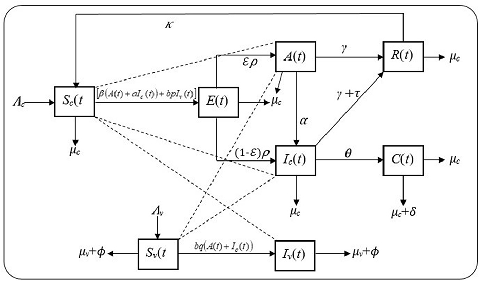
Figure 1. Schematic diagram showing the dynamics of mastitis in cattle and fly populations.

2.2. Model's assumptions

Other assumptions on which the model's formulation is based are as follows:

  i. Both populations are assumed not to be constant since births, immigrations, emigrations, and deaths occur in the populations.

 ii. The model assumes a homogeneous mixing of individuals in both populations where all individuals have an equal likelihood of contracting mastitis if they come into effective contact with infectious individuals, and that transmission of the infection occurs with a mass action incidence.

iii. The probability of survival till the infectious state for cattle exposed to mastitis is less than or equal to unity. As a result, the exposed class of cattle is included in the model for the cattle population but ignored for the fly population since flies generally have a short lifecycle.

iv. The chronic infective cows are assumed not to transmit mastitis because they are weak and, therefore, are culled from the herd at a rate, d.

 v. Mastitis-induced deaths of cows only occur at the chronic stage of the infection at a rate δ. The flies also experience induced deaths, at a rate ϕ, due to the application of insecticides such as methoprene, synthetic pyrethroids, organophosphates, and abamectins [9].

vi. Individual cattle who recover from mastitis, spontaneously or as a result of treatment via systemic and intramammary administration of antibiotics, supportive fluid, and anti-inflammatory therapy [4], lose their immunity, and become susceptible since mastitis is not known to confer permanent immunity.

From the schematic diagram in Figure 1 together with the set of the model's assumptions, the model is formulated as a system of ordinary differential equations, using the mass action incidence rate, as given in Equation (3).

$\begin{array}{ll}\begin{array}{l}\frac{d{S}_c\left(t\right)}{dt}={\Lambda }_c-\left[\beta \left(A\left(t\right)+a{I}_c\left(t\right)\right)+bp{I}_v\left(t\right)\right]S_c\left(t\right)-{\mu }_c{S}_c\left(t\right)+\kappa R\left(t\right)\\ \frac{dE\left(t\right)}{dt}=\left[\beta \left(A\left(t\right)+a{I}_c\left(t\right)\right)+bp{I}_v\left(t\right)\right]S_c\left(t\right)-\left({\mu }_c+\rho \right)E\left(t\right)\\ \frac{dA\left(t\right)}{dt}=\epsilon \rho E\left(t\right)-\left({\mu }_c+\alpha +\gamma \right)A\left(t\right)\\ \frac{d{I}_c\left(t\right)}{dt}=\left(1-\epsilon \right)\rho E\left(t\right)+\alpha A\left(t\right)-\left({\mu }_c+\theta +\gamma +\tau \right)I_c\left(t\right)\\ \frac{dC\left(t\right)}{dt}=\theta I_c\left(t\right)-\left({\mu }_c+\delta +d\right)C\left(t\right)\\ \frac{dR\left(t\right)}{dt}=\gamma A\left(t\right)+\left(\gamma +\tau \right)I_c\left(t\right)-\left({\mu }_c+\kappa \right)R\left(t\right)\\ \frac{d{S}_v\left(t\right)}{dt}={\Lambda }_v-bq\left(A\left(t\right)+I_c\left(t\right)\right)S_v\left(t\right)-\left({\mu }_v+\varphi \right)S_v\left(t\right)\\ \frac{d{I}_v\left(t\right)}{dt}=bq\left(A\left(t\right)+I_c\left(t\right)\right)S_v\left(t\right)-\left({\mu }_v+\varphi \right)I_v\left(t\right);\end{array}\}& (3)\end{array}$

subject to the initial conditions:

$\begin{array}{l}{S}_c\left(0\right)=S_{c_0},E\left(0\right)=E_0,A\left(0\right)=A_0,I_c\left(0\right)=I_{c_0},C\left(0\right)=C_0,\\ R\left(0\right)=R_0,S_v\left(0\right)=S_{v_0},I_v\left(0\right)=I_{v_0}.& (4)\end{array}$

The feasible region for the model is Ω = Ω₁ ∪ Ω₂, where

${\Omega }_1=\{\left(S_c\left(t\right),E\left(t\right),A\left(t\right),I_c\left(t\right),C\left(t\right),R\left(t\right)\right)ϵ{ℝ}_{+}^6:S_c\left(t\right)$ + E(t) + A(t) + I_c(t) + C(t) + R(t) = N_c(t)} and ${\Omega }_2=\left\{\left(S_v\left(t\right),I_v\left(t\right)\right)ϵ{ℝ}_{+}^2:S_v\left(t\right)+I_v\left(t\right)=N_c\left(t\right)\right\}$ are the region of feasibility for cattle and fly populations, respectively.

The parameters of the model are described in Table 1.

TABLE 1

Table 1. Description of the model's parameters.

2.3. Positivity and boundedness of solutions of the model

Theorem 1: Suppose the initial conditions (4) of the state variables are non-negative in the region Ω = Ω₁ ∪ Ω₂, then the solutions set {S_c(t), E(t), A(t), I_c(t), C(t), R(t), N_c(t)} ∈ Ω₁ and {S_v(t), I_v(t), N_v(t)} ∈ Ω₂ are non-negative in the region Ω for all time t ≥ 0.

Proof: It follows from the first equation of the model (3) that

$\begin{array}{l}\frac{d{S}_c\left(t\right)}{dt}\ge -\left[{\mu }_c+\beta \left(A\left(t\right)+a{I}_c\left(t\right)\right)+bp{I}_v\left(t\right)\right]S_c\left(t\right).\end{array}$

Separating the variables and integrating both sides gives

$\begin{array}{l}ln{S}_c\left(t\right)\ge -{\displaystyle \int }\left[{\mu }_c+\beta \left(A\left(t\right)+a{I}_c\left(t\right)\right)+bp{I}_v\left(t\right)\right]dt\\ \Rightarrow S_c\left(t\right)\ge A_1{e}^{-\left[{\mu }_{c}t+\int \left(\beta \left(A\left(t\right)+a{I}_c\left(t\right)\right)+bp{I}_v\left(t\right)\right)dt\right]}.\\ S\left(0\right)=S_0\Rightarrow A_1=S_0.\\ \therefore S_c\left(t\right)\ge S_0{e}^{-\left[{\mu }_{c}t+\int \left(\beta \left(A\left(t\right)+a{I}_c\left(t\right)\right)+bp{I}_v\left(t\right)\right)dt\right]}\\ \text{Thus }{S}_c\left(t\right)\ge 0,\text{ provided that }{S}_0\ge 0.\end{array}$

Similarly, it can be shown that E(t), A(t), I_c(t), C(t), R(t), S_v(t) and I_v(t) are non-negative. Hence, all the state variables are non-negative for all time t ≥ 0, whenever the initial conditions are non-negative.

Theorem 2: Every solution in the region Ω = Ω₁ ∪ Ω₂ are positively invariant with respect to the mastitis model (3) in cattle and fly populations.

Proof: Differentiating (1) and then substituting the first six equations of the model (3) gives,

$\begin{array}{l}\begin{array}{l}\frac{d{N}_c\left(t\right)}{dt}={\Lambda }_c-{\mu }_c{N}_c\left(t\right)-\left(\delta +d\right)C\left(t\right)\\ \Rightarrow \frac{d{N}_c\left(t\right)}{dt}\le {\Lambda }_c-{\mu }_c{N}_c\left(t\right)\\ \Rightarrow \frac{d{N}_c\left(t\right)}{dt}+{\mu }_c{N}_c\left(t\right)\le {\Lambda }_c\\ N\left(0\right)=N_0\Rightarrow A_2=N_0-\frac{{\Lambda }_c}{{\mu }_c}.\end{array}\end{array}$

Solving, using the integration factor, $I.F=e^{\int {\mu }_{c}dt}$, gives,

$\begin{array}{l}\begin{array}{l}\Rightarrow N_c\left(t\right)\le e^{-{\mu }_{c}t}\left[\int {\Lambda }_c{e}^{{\mu }_{c}t}dt\right]\\ \Rightarrow N_c\left(t\right)\le e^{-{\mu }_{c}t}\left[\frac{{\Lambda }_c}{{\mu }_c}{e}^{{\mu }_{c}t}+A_2\right]\\ \Rightarrow N_c\left(t\right)\le \frac{{\Lambda }_c}{{\mu }_c}+A_2{e}^{-{\mu }_{c}t}.\\ N\left(0\right)=N_0\Rightarrow A_2=N_0-\frac{{\Lambda }_c}{{\mu }_c}.\\ N_c\left(t\right)\le \frac{{\Lambda }_c}{{\mu }_c}+\left(N_0-\frac{{\Lambda }_c}{{\mu }_c}\right)e^{-{\mu }_{c}t}.\end{array}\end{array}$

$Ast\to 0,N_c\left(t\right)\to N_0$ and As $t\to \infty ,N_c\left(t\right)\to \frac{{\Lambda }_c}{{\mu }_c}$

$\mathrm{\text{Thus}}0\le N_c\left(t\right)\le \frac{{\Lambda }_c}{{\mu }_c}$.

Moreover, differentiating (2) and substituting the last two equations of the model (3) and then following the above procedures give $0\le N_v\left(t\right)\le \frac{{\Lambda }_v}{\left({\mu }_v+\varphi \right)}$.

These results imply that the mastitis model (3) has non-negative and bounded solutions in the region Ω = Ω₁ ∪ Ω₂, ∀t ≥ 0. Hence, the proposed mastitis model is both epidemiologically feasible and mathematically well-posed, and so, it suffices to consider the dynamics of the model in the feasible region Ω.

3. Analysis of the model

In this section, the mastitis model (3) is analyzed as follows: the equilibrium points and the effective reproduction number were obtained. Moreover, the local and global stabilities for both equilibria were investigated, and a sensitivity analysis was carried out.

3.1. Equilibria and effective reproduction number

Equilibrium points are steady-state solutions of the model satisfying

$\begin{array}{ll}\frac{d{S}_c\left(t\right)}{dt}=\frac{dE\left(t\right)}{dt}=...=\frac{d{I}_v\left(t\right)}{dt}=0.& (5)\end{array}$

3.1.1. Mastitis-free equilibrium

In the absence of mastitis, i.e., when E(t) = A(t) = I_c(t) = C(t) = I_v(t) = 0, then both cattle and fly populations are in a state of mastitis-free equilibrium, E₀, obtained by solving the model equation (3) subject to (5) and E(t) = A(t) = I_c(t) = C(t) = I_v(t) = 0 as follows:

$\begin{array}{ll}{E}_0=\left(\frac{{\Lambda }_c}{{\mu }_c},0,0,0,0,0,\frac{{\Lambda }_v}{\left({\mu }_c+\varphi \right)},0\right).& (6)\end{array}$

3.1.2. Effective reproduction number

The effective reproduction number, ℜ_c, is the actual average of secondary cases per primary case observed in a population with an infectious disease in the presence of control measures. Using the next generation operator, described by [15, 16],

$\begin{array}{ll}{\Re }_c=\rho \left(F{V}^{-1}\right)& (7)\end{array}$

where F is the Jacobian of the transmission matrix, obtained at E₀ as

$\begin{array}{ll}F=\left(\begin{array}{ccccc}0& \frac{\beta {\Lambda }_c}{{\mu }_c}& \frac{a\beta {\Lambda }_c}{{\mu }_c}& 0& \frac{bp{\Lambda }_c}{{\mu }_c}\\ 0& 0& 0& 0& 0\\ 0& 0& 0& 0& 0\\ 0& 0& 0& 0& 0\\ 0& \frac{bq{\Lambda }_v}{\left({\mu }_v+\varphi \right)}& \frac{bq{\Lambda }_v}{\left({\mu }_v+\varphi \right)}& 0& 0\end{array}\right),& (8)\end{array}$

and V is the Jacobian of the transition matrix, obtained at E₀ as

$\begin{array}{ll}V=\left(\begin{array}{ccccc}{\mu }_c+\rho & 0& 0& 0& 0\\ -\epsilon \rho & {\mu }_c+\alpha +\gamma & 0& 0& 0\\ -\left(1-\epsilon \right)\rho & -\alpha & {\mu }_c+\theta +\gamma +\tau & 0& 0\\ 0& 0& -\theta & {\mu }_c+\delta +d& 0\\ 0& 0& 0& 0& {\mu }_v+\varphi \end{array}\right),& (9)\end{array}$

Therefore, by (7), the effective reproduction number is the leading eigenvalue of the matrix FV⁻¹, computed as

$\begin{array}{l}{\Re }_c=\frac{\beta {\Lambda }_c}{2{\mu }_c{k}_1}\left[\frac{\epsilon \rho }{k_2}+\frac{a}{k_3}\left(\frac{\epsilon \rho \alpha }{k_2}+\left(1-\epsilon \right)\rho \right)\right]\\ +\sqrt{{\left\{\frac{\beta {\Lambda }_c}{2{\mu }_c{k}_1}\left[\frac{\epsilon \rho }{k_2}+\frac{a}{k_3}\left(\frac{\epsilon \rho \alpha }{k_2}+\left(1-\epsilon \right)\rho \right)\right]\right\}}^2+\frac{b^{2}pq{\Lambda }_c{\Lambda }_v}{{\mu }_c\left({\mu }_v+\varphi \right)k_1{k}_5}\left[\frac{\epsilon \rho }{k_2}+\frac{1}{k_3}\left(\frac{\epsilon \rho \alpha }{k_2}+\left(1-\epsilon \right)\rho \right)\right]},& (10)\end{array}$

where k₁ = μ_c + ρ, k₂ = μ_c + α + γ, k₃ = μ_c + θ + γ + τ, k₄ = μ_c + δ+d, and k₅ = μ_v + ϕ.

This can be summarized as

$\begin{array}{ll}{\Re }_c=\frac{1}{2}{\Re }_c^h+\sqrt{{\left(\frac{1}{2}{\Re }_c^h\right)}^2+{\Re }_c^v},& (11)\end{array}$

where ${\Re }_c^h=\frac{\beta {\Lambda }_c}{{\mu }_c{k}_1}\left[\frac{\epsilon \rho }{k_2}+\frac{a}{k_3}\left(\frac{\epsilon \rho \alpha }{k_2}+\left(1-\epsilon \right)\rho \right)\right]$ and ${\Re }_c^v=\frac{b^{2}pq{\Lambda }_c{\Lambda }_v}{{\mu }_c\left({\mu }_v+\varphi \right)k_1{k}_5}\left[\frac{\epsilon \rho }{k_2}+\frac{1}{k_3}\left(\frac{\epsilon \rho \alpha }{k_2}+\left(1-\epsilon \right)\rho \right)\right]$ represent the reproduction numbers for cattle–cattle transmission and fly–cattle transmission, respectively.

3.1.3. Mastitis-endemic equilibrium

In the presence of mastitis disease, i.e., when E(t) ≠ A(t) ≠ I_c(t) ≠ C(t) ≠ I_v(t) ≠ 0, then both cattle and fly populations are said to be in a state of mastitis-endemic equilibrium, E_e, obtained by solving (3) subject to (5) and E(t) ≠ A(t) ≠ I_c(t) ≠ C(t) ≠ I_v(t) ≠ 0 as

$\begin{array}{ll}{E}_e=\left(S_c^{*}\left(t\right),E^{*}\left(t\right),A^{*}\left(t\right),I_c^{*}\left(t\right),C^{*}\left(t\right),R^{*}\left(t\right),S_v^{*}\left(t\right),I_v^{*}\left(t\right)\right),& (12)\end{array}$

where $S_c^{*}\left(t\right)=\frac{1}{{\mu }_c}\{{\Lambda }_c+\frac{\kappa }{k_6}\left[\frac{\epsilon \rho \gamma }{k_2}+\frac{\gamma +\tau }{k_3}\left(\frac{\epsilon \rho \alpha }{k_2}+\left(1-\epsilon \right)\rho \right)-k_1\right]$ E^*(t)};

$\begin{array}{l}{A}^{*}\left(t\right)=\frac{\epsilon \rho }{k_2}{E}^{*}\left(t\right);\\ I_c^{*}\left(t\right)=\frac{1}{k_3}\left(\frac{\epsilon \rho \alpha }{k_2}+\left(1-\epsilon \right)\rho \right)E^{*}\left(t\right);\\ C^{*}\left(t\right)=\frac{\theta }{k_3{k}_4}\left(\frac{\epsilon \rho \alpha }{k_2}+\left(1-\epsilon \right)\rho \right)E^{*}\left(t\right);\\ R^{*}\left(t\right)=\frac{1}{k_6}\left[\frac{\epsilon \rho \gamma }{k_2}+\frac{\gamma +\tau }{k_3}\left(\frac{\epsilon \rho \alpha }{k_2}+\left(1-\epsilon \right)\rho \right)\right]E^{*}\left(t\right);\\ S_v^{*}\left(t\right)=\frac{{\Lambda }_v}{k_5}-I_v^{*}\left(t\right);\\ I_v^{*}\left(t\right)=\frac{{\Lambda }_v\left[\frac{\epsilon \rho }{k_2}+\frac{1}{k_3}\left(\frac{\epsilon \rho \alpha }{k_2}+\left(1-\epsilon \right)\rho \right)\right]E^{*}\left(t\right)}{1+\frac{\epsilon \rho }{k_2}+\frac{1}{k_3}\left(\frac{\epsilon \rho \alpha }{k_2}+\left(1-\epsilon \right)\rho \right)E^{*}\left(t\right)};\end{array}$

and E^*(t) is obtained as the roots of the quadratic equation

$\begin{array}{ll}A{E^{*}}^2\left(t\right)+B{E}^{*}\left(t\right)+C=0,& (13)\end{array}$

or equivalently, using the approach of [17]

$\begin{array}{l}{A}_1\left({\Re }_c^v-1\right){E^{*}}^2\left(t\right)+\left[k_5+B_1\left({\Re }_c^h-1\right)+B_2\left({\Re }_c^v-1\right)\right]E^{*}\left(t\right)\\ +k_5\left[\left({\Re }_c^h+{\Re }_c^v\right)-1\right]=0,& (14)\end{array}$

with positive constants A₁, B₁, and B₂ defined as follows:

$\begin{array}{l}{A}_1=\frac{\kappa bq\beta }{k_3{k}_6}\left[\frac{\epsilon \rho }{k_2}+\frac{1}{k_3}\left(\frac{\epsilon \rho \alpha }{k_2}+\left(1-\epsilon \right)\rho \right)\right][\frac{\epsilon \rho \gamma }{k_2}\\ +\frac{\gamma +\tau }{k_3}\left(\frac{\epsilon \rho \alpha }{k_2}+\left(1-\epsilon \right)\rho \right)];\\ B_1=bq\left[\frac{\epsilon \rho }{k_2}+\frac{1}{k_3}\left(\frac{\epsilon \rho \alpha }{k_2}+\left(1-\epsilon \right)\rho \right)\right];\text{ and}\\ B_2=\frac{1}{k_6}\left[\frac{\epsilon \rho \gamma }{k_2}+\frac{\gamma +\tau }{k_3}\left(\frac{\epsilon \rho \alpha }{k_2}+\left(1-\epsilon \right)\rho \right)\right];\end{array}$

so that the coefficients of (13) are given as

$\begin{array}{l}A=A_1\left({\Re }_c^v-1\right),B=\left[k_5+B_1\left({\Re }_c^h-1\right)+B_2\left({\Re }_c^v-1\right)\right],\text{and}\\ C=k_5\left\{\left({\Re }_c^h+{\Re }_c^v\right)-1\right\}.\end{array}$

We will now explore different cases of the mastitis-endemic equilibrium with respect to conditions placed on $A_1,B_1,B_2,{\Re }_c^h,{\Re }_c^v\text{ and }\left({\Re }_c^h+{\Re }_c^v\right)$ as follows:

  i. If ${\Re }_c^h<1,{\Re }_c^v<1\text{ and }\left({\Re }_c^h+{\Re }_c^v\right)>1$; then there exists a unique mastitis-endemic equilibrium;

 ii. If ${\Re }_c^h<1,{\Re }_c^v<1,\left({\Re }_c^h+{\Re }_c^v\right)=1\text{ and }\frac{c}{k_5}\left(B_1+B_2\right)<1,$ where c is a constant; then the model has two endemic equilibria, such that $E^{*}\left(t\right)=0or{E}^{*}\left(t\right)=\frac{k_5}{B_1}\left[1-\frac{c}{k_5}\left(B_1+B_2\right)\right]$;

iii. If ${\Re }_c^h<1,{\Re }_c^v<1,\left({\Re }_c^h+{\Re }_c^v\right)<1\text{ and }\frac{c}{k_5}\left(B_1+B_2\right)<1,$ where c is a constant; then the model has two endemic equilibria, one of which might coincide with the mastitis-free equilibrium;

iv. If ${\Re }_c^h>1,{\Re }_c^v>1,\text{ and }\left({\Re }_c^h+{\Re }_c^v\right)>1$; then there exists no endemic equilibria for the mastitis model;

 v. If ${\Re }_c^h>1,{\Re }_c^v>1,\text{ and }\left({\Re }_c^h+{\Re }_c^v\right)>1$; then the model has two distinct endemic equilibria.

3.2. Local asymptotic stability of the mastitis-free equilibrium

Theorem 3: If the sum $\left({\Re }_c^h+{\Re }_c^v\right)<1$, and the quantities $\frac{\beta {\Lambda }_c\left[\epsilon \rho +\left(1-\epsilon \right)\rho \right]}{{\mu }_c\left[k_1{k}_2+k_3{k}_5+\left(k_1+k_2\right)\left(k_3+k_5\right)\right]}<1$ and $\frac{\beta {\Lambda }_c\left(k_3+k_5\right)\left[\epsilon \rho +\left(\frac{\epsilon \rho \alpha }{\left(k_3+k_5\right)}+\left(1-\epsilon \right)\rho \right)\right]+b^{2}pq{\Lambda }_c{\Lambda }_v\epsilon \rho }{{\mu }_c\left[k_1{k}_2\left(k_3+k_5\right)+\left(k_1+k_2\right)k_3{k}_5\right]}<1,$ then the mastitis-free equilibrium is locally asymptotically stable. Otherwise, it is a saddle point that is unstable.

Proof: The stability of the mastitis-free equilibrium depends on the Jacobian matrix of the mastitis model (3), evaluated at E₀ as

$\begin{array}{ll}J{|}_{E_0}=\left(\begin{array}{cccccccc}-\left({\mu }_c+\lambda \right)& 0& -\frac{\beta {\Lambda }_c}{{\mu }_c}& -\frac{a\beta {\Lambda }_c}{{\mu }_c}& 0& \kappa & 0& -\frac{bp{\Lambda }_c}{{\mu }_c}\\ 0& -\left(k_1+\lambda \right)& \frac{\beta {\Lambda }_c}{{\mu }_c}& \frac{a\beta {\Lambda }_c}{{\mu }_c}& 0& 0& 0& \frac{bp{\Lambda }_c}{{\mu }_c}\\ 0& \epsilon \rho & -\left(k_2+\lambda \right)& 0& 0& 0& 0& 0\\ 0& \left(1-\epsilon \right)\rho & \alpha & -\left(k_3+\lambda \right)& 0& 0& 0& 0\\ 0& 0& 0& \theta & -\left(k_4+\lambda \right)& 0& 0& 0\\ 0& 0& \gamma & \gamma +\tau & 0& -\left(k_6+\lambda \right)& 0& 0\\ 0& 0& -\frac{bq{\Lambda }_v}{\left({\mu }_v+\varphi \right)}& -\frac{bq{\Lambda }_v}{\left({\mu }_v+\varphi \right)}& 0& 0& -\left(k_5+\lambda \right)& 0\\ 0& 0& \frac{bq{\Lambda }_v}{\left({\mu }_v+\varphi \right)}& \frac{bq{\Lambda }_v}{\left({\mu }_v+\varphi \right)}& 0& 0& 0& -\left(k_5+\lambda \right)\end{array}\right),& (15)\end{array}$

This has eigenvalues λ = −μ_c, λ = −k₄, λ = −k₅, λ = −k₆; others being the roots of the quartic equation (16) as follows:

$\begin{array}{l}{\lambda }^4+\left(k_1+k_2+k_3+k_5\right){\lambda }^3\\ +\left[k_1{k}_2+k_3{k}_5+\left(k_1+k_2\right)\left(k_3+k_5\right)\right]\left[1-R_1\right]{\lambda }^2\\ +\left[k_1{k}_2\left(k_3+k_5\right)+\left(k_1+k_2\right)k_3{k}_5\right]\left[1-R_2\right]\lambda \\ +k_1{k}_2{k}_3{k}_5\left[1-\left({\Re }_c^h+{\Re }_c^v\right)\right]=0.,& (16)\end{array}$

where

$\begin{array}{l}{R}_1=\frac{\beta {\Lambda }_c\left[\epsilon \rho +\left(1-\epsilon \right)\rho \right]}{{\mu }_c\left[k_1{k}_2+k_3{k}_5+\left(k_1+k_2\right)\left(k_3+k_5\right)\right]},\\ R_2=\frac{\beta {\Lambda }_c\left(k_3+k_5\right)\left[\epsilon \rho +\left(\frac{\epsilon \rho \alpha }{\left(k_3+k_5\right)}+\left(1-\epsilon \right)\rho \right)\right]+b^{2}pq{\Lambda }_c{\Lambda }_v\epsilon \rho }{{\mu }_c\left[k_1{k}_2\left(k_3+k_5\right)+\left(k_1+k_2\right)k_3{k}_5\right]}.\end{array}$

Now, if $\left({\Re }_c^h+{\Re }_c^v\right)<1$, and the quantities R₁ and R₂ are both less than unity, then the quartic equation (16) has negative roots or complex roots with negative real parts. Hence, the mastitis-free equilibrium is locally asymptotically stable. Otherwise, it is unstable.

3.3. Local asymptotic stability of the mastitis-endemic equilibria

In Section 3.1.3, we established that the mastitis model has some cases of the existence of endemic equilibrium. Of interest are the cases with unique (one) and two endemic equilibria. When two endemic equilibria exist (especially in cases (ii) and (iii) of Section 3.1.3), then this might cause the mastitis model to exhibit a subcritical (backward) bifurcation in which case a stable endemic equilibrium co-exists with stable disease-free equilibrium for ℜ_c < 1. When this happens, then, we have the occurrence of bi-stability [18, 19] as a result of backward bifurcation and the condition ℜ_c < 1 is a necessary but not a sufficient condition to eradicate mastitis in both cattle and the fly populations [20]. The condition for the existence of this backward bifurcation is described in the result of Theorem 4. When only one equilibrium exists, it is unique and the stabilities of this unique endemic equilibrium are established in Theorem 4 and Theorem 6.

Theorem 4: If ℜ_c ≥ 1, then the mastitis-endemic equilibrium is locally asymptotically stable. Otherwise, it is unstable.

Proof: The center manifold theory approach, described by Castillo–Chavez and Song [21, 22], is employed to establish the local asymptotic stability of the mastitis-endemic equilibrium around ℜ_c = 1.

From (11), we have,

$\begin{array}{l}{\Re }_c=\frac{1}{2}{\Re }_c^h+\sqrt{{\left(\frac{1}{2}{\Re }_c^h\right)}^2+{\Re }_c^v}.\end{array}$

Let β = β^*, where β^* is the chosen bifurcation parameter at ℜ_c = 1.

$\begin{array}{l}1=\frac{1}{2}{\Re }_c^h+\sqrt{{\left(\frac{1}{2}{\Re }_c^h\right)}^2+{\Re }_c^v}\\ \Rightarrow 1={\Re }_c^h+{\Re }_c^v\\ \Rightarrow 1=\frac{{\beta }^{*}{\Lambda }_c}{{\mu }_c{k}_1}\left[\frac{\epsilon \rho }{k_2}+\frac{a}{k_3}\left(\frac{\epsilon \rho \alpha }{k_2}+\left(1-\epsilon \right)\rho \right)\right]\\ +\frac{b^{2}pq{\Lambda }_c{\Lambda }_v}{{\mu }_c\left({\mu }_v+\varphi \right)k_1{k}_5}\left[\frac{\epsilon \rho }{k_2}+\frac{1}{k_3}\left(\frac{\epsilon \rho \alpha }{k_2}+\left(1-\epsilon \right)\rho \right)\right]\\ \Rightarrow {\beta }^{*}=\frac{{\mu }_c{k}_1}{{\Lambda }_c\left[\frac{\epsilon \rho }{k_2}+\frac{a}{k_3}\left(\frac{\epsilon \rho \alpha }{k_2}+\left(1-\epsilon \right)\rho \right)\right]}-\frac{b^{2}pq{\Lambda }_v}{\left({\mu }_v+\varphi \right)k_1{k}_5}.,\end{array}$

so that the mastitis-free equilibrium is locally asymptotically stable if $\beta <{\beta }^{*},\mathrm{\text{i.e. if }}{\Re }_c<1$, and unstable whenever $\beta >{\beta }^{*},\text{i.e. if }{\Re }_c>1$.

Now, let S_c(t) = x₁, E(t) = x₂, A(t) = x₃, I_c(t) = x₄, C(t) = x₅, R(t) = x₆, S_v(t) = x₇, I_v(t) = x₈, then the model in terms of these new state variables becomes

$\begin{array}{ll}\begin{array}{l}\frac{d{x}_1}{dt}=f_1={\Lambda }_c-\left[\beta \left(x_3+a{x}_4\right)+bp{x}_8\right]x_1-{\mu }_c{x}_1+\kappa x_6\\ \frac{d{x}_2}{dt}=f_2=\left[\beta \left(x_3+a{x}_4\right)+bp{x}_8\right]x_1-\left({\mu }_c+\rho \right)x_2\\ \frac{d{x}_3}{dt}=f_3=\epsilon \rho x_2-\left({\mu }_c+\alpha +\gamma \right)x_3\\ \frac{d{x}_4}{dt}=f_4=\left(1-\epsilon \right)\rho x_2+\alpha x_3-\left({\mu }_c+\theta +\gamma +\tau \right)x_4\\ \frac{d{x}_5}{dt}=f_5=\theta x_4-\left({\mu }_c+\delta +d\right)x_5\\ \frac{d{x}_6}{dt}=f_6=\gamma x_3+\left(\gamma +\tau \right)x_4-\left({\mu }_c+\kappa \right)x_6\\ \frac{d{x}_7}{dt}=f_7={\Lambda }_v-bq\left(x_3+x_4\right)x_7-\left({\mu }_v+\varphi \right)x_7\\ \frac{d{x}_8}{dt}=f_8=bq\left(x_3+x_4\right)x_7-\left({\mu }_v+\varphi \right)x_8.\end{array}\}& (17)\end{array}$

The Jacobian matrix of the model (17) at the mastitis-free equilibrium, E₀, when $\beta ={\beta }^{*},\text{ such that }{\Re }_c=1$, is obtained as in (15) with the calculated eigenvalues. If ℜ_c = 1, this implies that ${\Re }_c^h+{\Re }_c^v=1$. Then, the quartic equation (16) has a zero eigenvalue λ = 0; with other eigenvalues being negative.

Applying the center manifold theory, let $w={\left(w_1,w_2,w_3,...,w_8\right)}^T$ be the right eigenvector associated with the zero eigenvalues, λ = 0, where

$\begin{array}{l}{w}_1=-\frac{w_2}{{\mu }_c}\{\frac{{\beta }^{*}{\Lambda }_c}{{\mu }_c}\left[\frac{\epsilon \rho }{k_2}+\frac{a}{k_3}\left(\frac{\epsilon \rho \alpha }{k_2}+\left(1-\epsilon \right)\rho \right)\right]\\ -\frac{\kappa }{k_6}\left[\frac{\epsilon \rho \gamma }{k_2}+\frac{\theta \left(\gamma +\tau \right)}{k_3{k}_4}\left(\frac{\epsilon \rho \alpha }{k_2}+\left(1-\epsilon \right)\rho \right)\right]\\ +\frac{b^{2}pq{\Lambda }_c{\Lambda }_v}{{\mu }_c\left({\mu }_v+\varphi \right)k_1{k}_5}\left[\frac{\epsilon \rho }{k_2}+\frac{1}{k_3}\left(\frac{\epsilon \rho \alpha }{k_2}+\left(1-\epsilon \right)\rho \right)\right]\};\\ w_2=w_2>0\left(\text{afree eigenvector}\right);\\ w_3=\frac{\epsilon \rho }{k_2}{w}_2;\\ w_4=\frac{a}{k_3}\left(\frac{\epsilon \rho \alpha }{k_2}+\left(1-\epsilon \right)\rho \right)w_2;\\ w_5=\frac{\theta }{k_3{k}_4}\left(\frac{\epsilon \rho \alpha }{k_2}+\left(1-\epsilon \right)\rho \right)w_2;\\ w_6=\frac{w_2}{k_6}\left[\frac{\epsilon \rho \gamma }{k_2}+\frac{\theta \left(\gamma +\tau \right)}{k_3{k}_4}\left(\frac{\epsilon \rho \alpha }{k_2}+\left(1-\epsilon \right)\rho \right)\right];\\ w_7=-\frac{bq{\Lambda }_v}{\left({\mu }_v+\varphi \right)k_5}\left[\frac{\epsilon \rho }{k_2}+\frac{1}{k_3}\left(\frac{\epsilon \rho \alpha }{k_2}+\left(1-\epsilon \right)\rho \right)\right]w_2;\\ w_8=\frac{bq{\Lambda }_v}{\left({\mu }_v+\varphi \right)k_5}\left[\frac{\epsilon \rho }{k_2}+\frac{1}{k_3}\left(\frac{\epsilon \rho \alpha }{k_2}+\left(1-\epsilon \right)\rho \right)\right]w_2.\end{array}$

Similarly, the left eigenvector associated with the zero eigenvalues, λ = 0, is given by v = (v₁, v₂, v₃, ..., v₈), such that v. w = 1, where

$\begin{array}{l}{v}_1=v_5=v_6=v_7=0;\\ v_2=v_2>0\left(\text{a free eigenvector}\right);\\ v_3=\frac{{\Lambda }_c}{{\mu }_c{k}_2}\left(1-\frac{\alpha }{k_3}\right)\left[{\beta }^{*}+\frac{b^{2}pq{\Lambda }_v}{\left({\mu }_v+\varphi \right)k_5}\right]v_2;\\ v_4=\frac{{\Lambda }_c}{{\mu }_c{k}_3}\left[a{\beta }^{*}+\frac{b^{2}pq{\Lambda }_v}{\left({\mu }_v+\varphi \right)k_5}\right]v_2;\\ v_8=\frac{bp{\Lambda }_c}{{\mu }_c{k}_5}{v}_2.\end{array}$

Computation of a and b

The coefficients a and b as defined by Castillo–Chavez and Song [21] are $a={\displaystyle \sum _{k,i,j=1}^8}{v}_k{w}_i{w}_j\frac{{\partial }^2{f}_k\left(E_0,{\beta }^{*}\right)}{\partial x_i\partial x_j}$ $\text{ and }b={\displaystyle \sum _{k,i=1}^8}{v}_k{w}_i\frac{{\partial }^2{f}_k\left(E_0,{\beta }^{*}\right)}{\partial x_i\partial {\beta }^{*}}$; and are algebraically computed as follows, considering only the non-zero components f_k: k = 2, 3, 4, 8. With these definitions, the following was obtained:

$\begin{array}{l}a=2v_2{w}_1\left(w_3{\beta }^{*}+w_{4}a{\beta }^{*}+w_{8}bp\right)+2v_8{w}_{7}bq\left(w_3+w_4\right).\end{array}$

On substitution of necessary quantities and simplifying, the above reduces to

$\begin{array}{ll}a=-v_2{w}_2^2\frac{k_1}{{\Lambda }_c}{\left({\Re }_c^h+{\Re }_c^v\right)}^2\left(1-Q\right);& (18)\end{array}$

where $Q=\frac{\kappa }{{\Lambda }_c{k}_1{k}_6}\left[\frac{\epsilon \rho \gamma }{k_2}+\frac{\theta \left(\gamma +\tau \right)}{k_3{k}_4}\left(\frac{\epsilon \rho \alpha }{k_2}+\left(1-\epsilon \right)\rho \right)\right]$ $+\frac{{{\Re }_c^v}^2}{k_1{\left({\Re }_c^h+{\Re }_c^v\right)}^2}\left[\frac{\epsilon \rho }{k_2}+\frac{1}{k_3}\left(\frac{\epsilon \rho \alpha }{k_2}+\left(1-\epsilon \right)\rho \right)\right]$.

Similarly, the coefficient b is obtained as

$\begin{array}{l}b=v_2{x}_1\left(w_3+a{w}_4\right)\\ =v_2{w}_2\frac{{\Lambda }_c}{{\mu }_c}\left[\frac{\epsilon \rho }{k_2}+\frac{1}{k_3}\left(\frac{\epsilon \rho \alpha }{k_2}+\left(1-\epsilon \right)\rho \right)\right].& (19)\end{array}$

Thus b > 0, since v₂, w₂ > 0, and all parameters are positive.

Now, from (18), if the quantity Q < 1, then a < 1, b > 0, and the model exhibit a forward bifurcation around ℜ_c = 1; when β^* < 0, then there exists a positive stable equilibrium. This implies that the disease-free is globally stable while the endemic equilibrium is locally asymptotically stable when ℜ_c > 1, but close to 1. This scenario is depicted in Figure 2A, and in this case, the condition ℜ_c < 1 is sufficient to eradicate mastitis disease from the populations.

FIGURE 2

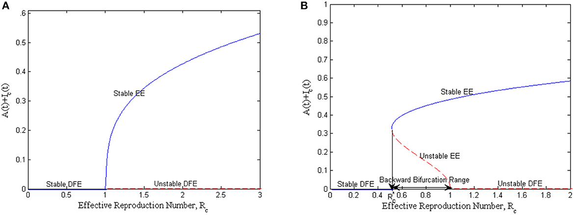
Figure 2. Bifurcation curve at the threshold value, ℜ_c = 1: (A) forward bifurcation plot and (B) backward bifurcation plot.

If, however, Q > 1, then a > 1, b > 0, and so the model exhibits a backward bifurcation at ℜ_c = 1; when β^* < 0, then x = 0 is unstable and there exists a negative and locally asymptotically stable endemic equilibrium. This implies that the disease-free is not globally stable while the endemic equilibrium is locally asymptotically stable, whenever ℜ_c > 1. This scenario is shown in Figure 2B, and in this case, the condition ℜ_c < 1 is not sufficient to eradicate mastitis in both populations. For mastitis disease to be curtailed or eradicated from the population, the condition ${\Re }_c^{*}<{\Re }_c<1$ must hold.

3.4. Global asymptotic stability of the equilibria

In this section, the global asymptotic stability of the mastitis-free and mastitis-endemic equilibrium are investigated. It should be noted that whenever a stable endemic equilibrium co-exists with the disease-free equilibrium (for the existence of backward bifurcation), then the mastitis-free equilibrium cannot be globally stable and the endemic equilibrium also might not be globally stable [18, 23, 24]. Given this, the global stabilities are considered for the case with unique endemic equilibrium or when Q < 1 in Section 3.3 above and the model exhibits a forward bifurcation.

3.4.1. Global asymptotic stability of the mastitis-free equilibrium

To show the global stability of the mastitis-free equilibria, the two conditions for the global stability of disease-free as contained in [25–27] for ℜ_c < 1 were established.

We begin by re-writing the model equation (3) in the form

$\begin{array}{l}\frac{dX}{dt}=F\left(X,Y\right)\text{ and }\frac{dY}{dt}=G\left(X,Y\right),G\left(X,0\right)=0;\end{array}$

where X = (S_c(t), R(t), S_c(t)) and Y = (E(t), A(t), I_c(t), C(t), I_v(t)) are the non-infectious and the infectious states of the system; F(X, Y) and G(X, Y) are the right-hand sides of $\stackrel{.}{X}$ and $\stackrel{.}{Y}$, respectively, with E(t) = A(t) = I_c(t) = C(t) = I_v(t) = 0.

Now, from the model (3), the reduced system $\frac{dX}{dt}=F\left(X,0\right)$ is given as

$\begin{array}{ll}\begin{array}{l}\frac{d{S}_c\left(t\right)}{dt}={\Lambda }_c-{\mu }_c{S}_c\left(t\right)+\kappa R\left(t\right)\\ \frac{dR\left(t\right)}{dt}=-\left({\mu }_c+\kappa \right)R\left(t\right)\\ \frac{d{S}_v\left(t\right)}{dt}={\Lambda }_v-\left({\mu }_v+\varphi \right)S_v\left(t\right);\end{array}& (20)\end{array}$

Let $X^{*}=\left(S_c^{*}\left(t\right),R^{*}\left(t\right),S_c^{*}\left(t\right)\right)=\left(\frac{{\Lambda }_c}{{\mu }_c},0,\frac{{\Lambda }_v}{\left({\mu }_c+\varphi \right)}\right)$ be the equilibrium of the reduced system (20) then the following result holds.

Theorem 5: The mastitis-free equilibrium, E₀, of the model (3) is globally asymptotically stable if ℜ_c < 1; provided that the conditions (H₁) and (H₂) below are satisfied:

H₁: For $\frac{dX}{dt}=F\left(X,0\right),X^{*}$ is globally asymptotically stable;

H₂: G(X, Y) = AY − Ĝ(X, Y), Ĝ(X, Y) ≥ 0 for (X, Y) ∈ Ω.

where $A=D_{Y}G\left(X^{*},0\right)$ is a Metzler matrix (the off-diagonal elements of A are non-negative) and Ω is the region where the model is biologically feasible.

Proof: First, we show that X^* is globally asymptotically stable by solving each equation in the reduced system (20) and then taking the limit as t → ∞.

Thus, solving the second equation in (20) subject to the initial condition R(0) = R₀ gives

$\begin{array}{ll}R\left(t\right)=R_0{e}^{-\left({\mu }_c+\kappa \right)t}.& (21)\end{array}$

As t → ∞, R(t) → 0, and independent of R₀.

Moreover, from the first equation in (20), we have that

$\begin{array}{l}\frac{d{S}_c\left(t\right)}{dt}+{\mu }_c{S}_c\left(t\right)={\Lambda }_c+\kappa R\left(t\right)\\ \Rightarrow \frac{d{S}_c\left(t\right)}{dt}+{\mu }_c{S}_c\left(t\right)={\Lambda }_c+\kappa R_0{e}^{-\left({\mu }_c+\kappa \right)t}.\end{array}$

Solving this with its integrating factor, $e^{{\mu }_{c}t}$, and subject to the initial condition S_c(0) = S_c0 gives

$\begin{array}{ll}{S}_c\left(t\right)=\frac{{\Lambda }_c}{{\mu }_c}\left(1-e^{-{\mu }_{c}t}\right)+S_{c_0}{e}^{-{\mu }_{c}t}+R_0\left(e^{-\left({\mu }_c+\kappa \right)t}-e^{-{\mu }_{c}t}\right).& (22)\end{array}$

$\text{As }t\to \infty ,S_c\left(t\right)\to \frac{{\Lambda }_c}{{\mu }_c}$, and independent of S_c0.

From the last equation in (20), we have,

$\begin{array}{l}\frac{d{S}_v\left(t\right)}{dt}+\left({\mu }_v+\varphi \right)S_v\left(t\right)={\Lambda }_v.\end{array}$

Solving this with its integrating factor, $e^{\left({\mu }_v+\varphi \right)t}$, and subject to the initial condition S_v(0) = S_v0 gives

$\begin{array}{ll}{S}_v\left(t\right)=\frac{{\Lambda }_v}{{\mu }_v+\varphi }+\left(S_{v_0}-\frac{{\Lambda }_v}{{\mu }_v+\varphi }\right)e^{-\left({\mu }_v+\varphi \right)t}.& (23)\end{array}$

$\text{As }t\to \infty ,S_v\left(t\right)\to \frac{{\Lambda }_v}{{\mu }_v+\varphi }$, and independent of S_v0.

This implies that the asymptotic dynamics of the system are independent of the initial conditions, i.e., every solution of the model with initial conditions in Ω approaches $X^{*}=E_0,\text{ as }t\to \infty$. Hence, the equilibrium X^* is globally asymptotically stable for $\frac{dX}{dt}=F\left(X,0\right)$.

Next, it is left to show H₂: G(X, Y) = AY − Ĝ(X, Y), Ĝ(X, Y) ≥ 0 for (X, Y) ∈ Ω.

From the model (3),

$\begin{array}{l}G\left(X,Y\right)=\left(\begin{array}{c}\left[\beta \left(A\left(t\right)+a{I}_c\left(t\right)\right)+bp{I}_v\left(t\right)\right]S_c\left(t\right)-\left({\mu }_c+\rho \right)E\left(t\right)\\ \epsilon \rho E\left(t\right)-\left({\mu }_c+\alpha +\gamma \right)A\left(t\right)\\ \left(1-\epsilon \right)\rho E\left(t\right)+\alpha A\left(t\right)-\left({\mu }_c+\theta +\gamma +\tau \right)I_c\left(t\right)\\ \theta I_c\left(t\right)-\left({\mu }_c+\delta +d\right)C\left(t\right)\\ bq\left(A\left(t\right)+I_c\left(t\right)\right)S_v\left(t\right)-\left({\mu }_v+\varphi \right)I_v\left(t\right)\end{array}\right);\end{array}$

and

$\begin{array}{l}A=D_{Y}G\left(X^{*},0\right)\\ =\left(\begin{array}{ccccc}-\left({\mu }_c+\rho \right)& \frac{\beta {\Lambda }_c}{{\mu }_c}& \frac{a\beta {\Lambda }_c}{{\mu }_c}& 0& \frac{bp{\Lambda }_c}{{\mu }_c}\\ \epsilon \rho & -\left({\mu }_c+\alpha +\gamma \right)& 0& 0& 0\\ \left(1-\epsilon \right)\rho & \alpha & -\left({\mu }_c+\theta +\gamma +\tau \right)& 0& 0\\ 0& 0& \theta & -\left({\mu }_c+\delta +d\right)& 0\\ 0& \frac{bq{\Lambda }_v}{\left({\mu }_v+\varphi \right)}& \frac{bq{\Lambda }_v}{\left({\mu }_v+\varphi \right)}& 0& -\left({\mu }_c+\varphi \right)\end{array}\right),\\ AY=\left(\begin{array}{ccccc}-\left({\mu }_c+\rho \right)& \frac{\beta {\Lambda }_c}{{\mu }_c}& \frac{a\beta {\Lambda }_c}{{\mu }_c}& 0& \frac{bp{\Lambda }_c}{{\mu }_c}\\ \epsilon \rho & -\left({\mu }_c+\alpha +\gamma \right)& 0& 0& 0\\ \left(1-\epsilon \right)\rho & \alpha & -\left({\mu }_c+\theta +\gamma +\tau \right)& 0& 0\\ 0& 0& \theta & -\left({\mu }_c+\delta +d\right)& 0\\ 0& \frac{bq{\Lambda }_v}{\left({\mu }_v+\varphi \right)}& \frac{bq{\Lambda }_v}{\left({\mu }_v+\varphi \right)}& 0& -\left({\mu }_c+\varphi \right)\end{array}\right)\left(\begin{array}{c}E\left(t\right)\\ A\left(t\right)\\ I_c\left(t\right)\\ C\left(t\right)\\ I_v\left(t\right)\end{array}\right)\\ =\left(\begin{array}{c}-\left({\mu }_c+\rho \right)E\left(t\right)+\frac{\beta {\Lambda }_c}{{\mu }_c}A\left(t\right)+\frac{a\beta {\Lambda }_c}{{\mu }_c}{I}_c\left(t\right)+\frac{bp{\Lambda }_c}{{\mu }_c}{I}_v\left(t\right)\\ \epsilon \rho E\left(t\right)+-\left({\mu }_c+\alpha +\gamma \right)A\left(t\right)\\ \left(1-\epsilon \right)\rho E\left(t\right)+\alpha A\left(t\right)-\left({\mu }_c+\theta +\gamma +\tau \right)I_c\left(t\right)\\ \theta I_c\left(t\right)-\left({\mu }_c+\delta +d\right)C\left(t\right)\\ \frac{bq{\Lambda }_v}{\left({\mu }_v+\varphi \right)}A\left(t\right)+\frac{bq{\Lambda }_v}{\left({\mu }_v+\varphi \right)}{I}_c\left(t\right)-\left({\mu }_c+\varphi \right)I_v\left(t\right)\end{array}\right).\end{array}$

Then G(X, Y) = AY − Ĝ(X, Y) implies Ĝ(X, Y) = AY − G(X, Y), so that

$\begin{array}{l}Ĝ\left(X,Y\right)=\left(\begin{array}{c}\left[\beta \left(A\left(t\right)+a{I}_c\left(t\right)\right)+bp{I}_v\left(t\right)\right]\left(\frac{{\Lambda }_c}{{\mu }_c}-S_c\left(t\right)\right)\\ 0\\ 0\\ 0\\ bq\left(A\left(t\right)+I_c\left(t\right)\right)\left(\frac{bq{\Lambda }_v}{\left({\mu }_v+\varphi \right)}-S_v\left(t\right)\right)\end{array}\right)\\ =\left(\begin{array}{c}{Ĝ}_1\left(X,Y\right)\\ {Ĝ}_2\left(X,Y\right)\\ {Ĝ}_3\left(X,Y\right)\\ {Ĝ}_4\left(X,Y\right)\\ {Ĝ}_5\left(X,Y\right)\end{array}\right).& (24)\end{array}$

Obviously, Ĝ₂(X, Y) = Ĝ₃(X, Y) = Ĝ₄(X, Y) = 0. Moreover, Ĝ₁(X, Y) ≥ 0 and Ĝ₅(X, Y) ≥ 0 since $S_c\left(t\right)\le \frac{{\Lambda }_c}{{\mu }_c}\text{ and }{S}_v\left(t\right)\le \frac{{\Lambda }_v}{{\mu }_v+\varphi }$ at any time t, as shown in H₁.

Now, it has been established that: (i) For $\frac{dX}{dt}=F\left(X,0\right),X^{*}$ is globally asymptotically stable; and

(ii) G(X, Y) = AY − Ĝ(X, Y), Ĝ(X, Y) ≥ 0 for (X, Y) ∈ Ω.

Hence, the mastitis-free equilibrium, E₀, is globally asymptotically stable whenever ℜ_c < 1, and unstable otherwise.

3.4.2. Global asymptotic stability of the mastitis-endemic equilibrium

Theorem 6: If ℜ_c > 1, then the mastitis-endemic equilibrium, whenever it is unique, is globally asymptotically stable in Ω, provided that $I_c\ge I_c^{*};C\ge C^{*};R\ge R^{*};S_c^{*}E\ge S_c{E}^{*};S_v^{*}{I}_v\ge S_v{I}_v^{*}$.

Proof: The global stability of the mastitis-endemic equilibrium is analyzed by constructing a suitable Lyapunov function V(t) of Goh–Volterra type, following the approach of [26–30], such that

$\begin{array}{l}V\left(t\right)=\left(S_c-S_c^{*}-S_c^{*}ln\frac{S_c}{S_c^{*}}\right)+\left(E-E^{*}-E^{*}ln\frac{E}{E^{*}}\right)\\ +K\left(A-A^{*}-A^{*}ln\frac{A}{A^{*}}\right)+\left(I_c-I_c^{*}-I_c^{*}ln\frac{I_c}{I_c^{*}}\right)\\ +\left(C-C^{*}-C^{*}\left(t\right)ln\frac{C}{C^{*}}\right)\\ +\frac{\kappa R^{*}}{\gamma A^{*}+\left(\gamma +\tau \right)I_c^{*}}\left(R-R^{*}-R^{*}ln\frac{R}{R^{*}}\right)\\ +\left(S_v-S_v^{*}-S_v^{*}ln\frac{S_v}{S_v^{*}}\right)+\left(I_v-I_v^{*}-I_v^{*}ln\frac{I_v}{I_v^{*}}\right),& (25)\end{array}$

where $K=\left[\frac{\beta \left(A^{*}+a{I}_c^{*}\right)+bp{I}_c^{*}}{\epsilon \rho E^{*}}\right]S_c^{*}$.

The time derivative of V(t) along the solutions of the system (3) is obtained as

$\begin{array}{l}\frac{dV\left(t\right)}{dt}=\left(1-\frac{S_c^{*}}{S_c}\right)\frac{d{S}_c}{dt}+\left(1-\frac{E^{*}}{E}\right)\frac{dE}{dt}+K\left(1-\frac{A^{*}}{A}\right)\frac{dA}{dt}\\ +\left(1-\frac{I_c^{*}}{I_c}\right)\frac{d{I}_c}{dt}+\left(1-\frac{C^{*}}{C}\right)\frac{dC}{dt}\\ +\frac{\kappa R^{*}}{\gamma A^{*}+\left(\gamma +\tau \right)I_c^{*}}\left(1-\frac{R^{*}}{R}\right)\frac{dR}{dt}\\ +\left(1-\frac{S_v^{*}}{S_v}\right)\frac{d{S}_v}{dt}+\left(1-\frac{I_v^{*}}{I_v}\right)\frac{d{I}_v}{dt}.\end{array}$

Putting the appropriate equations of the system (3) into the derivative of V(t) gives

$\begin{array}{l}\frac{dV\left(t\right)}{dt}-=\left(1-\frac{S_c^{*}}{S_c}\right)\left({\Lambda }_c-\left[\beta \left(A+a{I}_c\right)+bp{I}_v\right]S_c-{\mu }_c{S}_c+\kappa R\right)\\ +\left(1-\frac{E^{*}}{E}\right)\left(\left[\beta \left(A+a{I}_c\right)+bp{I}_v\right]S_c-\left({\mu }_c+\rho \right)E\right)\\ +K\left(1-\frac{A^{*}}{A}\right)\left(\epsilon \rho E-\left({\mu }_c+\alpha +\gamma \right)A\right)\\ +\left(1-\frac{I_c^{*}}{I_c}\right)\left(\left(1-\epsilon \right)\rho E+\alpha A-\left({\mu }_c+\theta +\gamma +\tau \right)I_c\right)\\ +\left(1-\frac{C^{*}}{C}\right)\left(\theta I_c-\left({\mu }_c+\delta +d\right)C\right)\\ +\frac{\kappa R^{*}}{\gamma A^{*}+\left(\gamma +\tau \right)I_c^{*}}\left(1-\frac{R^{*}}{R}\right)\left(\gamma A+\left(\gamma +\tau \right)I_c-\left({\mu }_c+\kappa \right)R\right)\\ +\left(1-\frac{S_v^{*}}{S_v}\right)\left({\Lambda }_v-bq\left(A+I_c\right)S_v-\left({\mu }_v+\varphi \right)S_v\right)\\ +\left(1-\frac{I_v^{*}}{I_v}\right)\left(bq\left(A+I_c\right)S_v-\left({\mu }_v+\varphi \right)I_v\right).& (26)\end{array}$

At the mastitis-endemic equilibria of the model, the following relationships hold from the model (3):

$\begin{array}{l}{\Lambda }_c=\left[\beta \left(A^{*}+a{I}_c^{*}\right)+bp{I}_v^{*}\right]S_c^{*}+{\mu }_c{S}_c^{*}-\kappa R^{*};\\ \left({\mu }_c+\rho \right)=\frac{\left[\beta \left(A^{*}+a{I}_c^{*}\right)+bp{I}_v^{*}\right]S_c^{*}}{E^{*}\left(t\right)};\\ \left({\mu }_c+\alpha +\gamma \right)=\frac{\epsilon \rho E^{*}}{A^{*}};\\ \left({\mu }_c+\theta +\gamma +\tau \right)=\frac{\left(1-\epsilon \right)\rho E^{*}+\alpha A^{*}}{I_c^{*}};\\ \left({\mu }_c+\delta +d\right)=\frac{\theta I_c^{*}}{C^{*}};\\ \left({\mu }_c+\kappa \right)=\frac{\gamma A^{*}+\left(\gamma +\tau \right)I_c^{*}}{R^{*}};\\ {\Lambda }_v=bq\left(A^{*}+I_c^{*}\right)S_v^{*}+\left({\mu }_v+\varphi \right)S_v^{*};\\ \left({\mu }_v+\varphi \right)=\frac{bq\left(A^{*}+I_c^{*}\right)S_v^{*}}{I_v^{*}}.\end{array}$

Using these relations in (26) yields

$\begin{array}{l}\frac{dV\left(t\right)}{dt}=\left(1-\frac{S_c^{*}}{S_c}\right)\{(\left[\beta \left(A^{*}+a{I}_c^{*}\right)+bp{I}_v^{*}\right]S_c^{*}\\ -\left[\beta \left(A+a{I}_c\right)+bp{I}_v\left(t\right)\right]S_c)+{\mu }_c\left(S_c^{*}-S_c\right)+\kappa \left(R-R^{*}\right)\}\\ +\left(1-\frac{E^{*}}{E}\right)(\left[\beta \left(A+a{I}_c\right)+bp{I}_v\right]S_c\\ -\left[\beta \left(A^{*}+a{I}_c^{*}\right)+bp{I}_v^{*}\right]\frac{S_c^{*}E}{E^{*}})\\ +S_c^{*}\left[\frac{\beta \left(A^{*}+a{I}_c^{*}\right)+bp{I}_c^{*}}{\epsilon \rho E^{*}}\right]\left(1-\frac{A^{*}}{A}\right)\left(\epsilon \rho E-\epsilon \rho \frac{E^{*}A}{A^{*}}\right)\\ +\left(1-\frac{I_c^{*}}{I_c}\right)\left(\left[\left(1-\epsilon \right)\rho E+\alpha A\right]-\left[\left(1-\epsilon \right)\rho E^{*}+\alpha A^{*}\right]\frac{I_c}{I_c^{*}}\right)\\ +\left(1-\frac{C^{*}}{C}\right)\left(\theta I_c-\theta \frac{I_c^{*}C}{C^{*}}\right)+\frac{\kappa R^{*}}{\gamma A^{*}+\left(\gamma +\tau \right)I_c^{*}}\left(1-\frac{R^{*}}{R}\right)\\ \left(\left[\gamma A+\left(\gamma +\tau \right)I_c\right]-\left[\gamma A^{*}+\left(\gamma +\tau \right)I_c^{*}\right]\frac{R}{R^{*}}\right)\\ +\left(1-\frac{S_v^{*}}{S_v}\right)(bq\left(A^{*}+I_c^{*}\right)S_v^{*}-bq\left(A+I_c\left(t\right)\right)S_v\\ +\left({\mu }_v+\varphi \right)\left[S_v^{*}-S_v\right])\\ +\left(1-\frac{I_v^{*}}{I_v}\right)\left(bq\left(A+I_c\left(t\right)\right)S_v-bq\left(A^{*}+I_c^{*}\right)\frac{S_v^{*}{I}_v}{I_v^{*}}\right).\end{array}$

Expanding and simplifying this gives

$\begin{array}{l}\frac{dV\left(t\right)}{dt}=S_c^{*}\left[\beta \left(A^{*}+a{I}_c^{*}\right)+bp{I}_v^{*}\right]\left\{3-\frac{S_c^{*}}{S_c}-\frac{A}{A^{*}}-\frac{A^{*}E}{A{E}^{*}}\right\}\\ +S_c\left[\beta \left(A+a{I}_c\right)+bp{I}_v\left(t\right)\right]\left\{1-\frac{S_c{E}^{*}}{S_c^{*}E}\right\}\\ +{\mu }_c\left(S_c^{*}-S_c\right)\left(1-\frac{S_c^{*}}{S_c}\right)+\kappa \left(R-R^{*}\right)\left(1-\frac{S_c^{*}}{S_c}\right)\\ +\left[\left(1-\epsilon \right)\rho E+\alpha A\right]\left(1-\frac{I_c^{*}}{I_c}\right)+\left[\left(1-\epsilon \right)\rho E^{*}+\alpha A^{*}\right]\left(1-\frac{I_c}{I_c^{*}}\right)\\ +\theta I_c^{*}\left\{1-\frac{C}{C^{*}}-\frac{C^{*}{I}_c}{C{I}_c^{*}}+\frac{I_c}{I_c^{*}}\right\}\\ +\kappa R^{*}\left\{1-\frac{R}{R^{*}}-\frac{\gamma A+\left(\gamma +\tau \right)I_c}{\gamma A^{*}+\left(\gamma +\tau \right)I_c^{*}}+\left[\frac{\gamma A+\left(\gamma +\tau \right)I_c}{\gamma A^{*}+\left(\gamma +\tau \right)I_c^{*}}\right]\frac{R^{*}}{R}\right\}\\ +bq{S}_v^{*}\left(A^{*}+I_c^{*}\right)\left\{2-\frac{S_v^{*}}{S_v}-\frac{I_v}{I_v^{*}}\right\}\\ +bq{S}_v\left(A+I_c\left(t\right)\right)\left\{1-\frac{S_v{I}_v^{*}}{S_v^{*}{I}_v}\right\}+S_v^{*}\left({\mu }_v+\varphi \right)\left\{2-\frac{S_v}{S_v^{*}}-\frac{S_v^{*}}{S_v}\right\}.\end{array}$

This simplifies to

$\begin{array}{ll}\begin{array}{l}\frac{dV\left(t\right)}{dt}=S_c^{*}\left[\beta \left(A^{*}+a{I}_c^{*}\right)+bp{I}_v^{*}\right]\{3-[\frac{S_c^{*}}{S_c}+\frac{A}{A^{*}}+\frac{A^{*}E}{A{E}^{*}}\\ -\frac{\beta \left(A+a{I}_c\right)+bp{I}_v}{\beta \left(A^{*}+a{I}_c^{*}\right)+bp{I}_v^{*}}\left(1-\frac{S_c{E}^{*}}{S_c^{*}E}\right)]\}\\ +bq{S}_v^{*}\left(A^{*}+I_c^{*}\right)\left\{2-\left[\frac{S_v^{*}}{S_v}+\frac{I_v}{I_v^{*}}-\frac{bq{S}_v\left(A+I_c\left(t\right)\right)}{bq{S}_v^{*}\left(A^{*}+I_c^{*}\right)}\left(1-\frac{S_v{I}_v^{*}}{S_v^{*}{I}_v}\right)\right]\right\}\\ +{\mu }_c{S}_c^{*}\left\{2-\left[\frac{S_c^{*}}{S_c}+\frac{S_c}{S_c^{*}}\right]\right\}\\ +S_v^{*}\left({\mu }_v+\varphi \right)\left\{2-\left[\frac{S_v}{S_v^{*}}-\frac{S_v^{*}}{S_v}\right]\right\}+\left[\left(1-\epsilon \right)\rho E^{*}+\alpha A^{*}\right]\\ \left\{1-\left[\frac{I_c}{I_c^{*}}-\frac{\left(1-\epsilon \right)\rho E+\alpha A}{\left(1-\epsilon \right)\rho E^{*}+\alpha A^{*}}\left(1-\frac{I_c^{*}}{I_c}\right)\right]\right\}\\ +\kappa R\left\{1-\left[\frac{S_c^{*}}{S_c}+\frac{R^{*}}{R}+\frac{S_c^{*}{R}^{*}}{S_{c}R}\right]\right\}\\ +\kappa R^{*}\left\{1-\left[\frac{R}{R^{*}}-\frac{\gamma A+\left(\gamma +\tau \right)I_c}{\gamma A^{*}+\left(\gamma +\tau \right)I_c^{*}}\left(1-\frac{R^{*}}{R}\right)\right]\right\}\\ +\theta I_c^{*}\left\{1-\left[\frac{C}{C^{*}}-\frac{I_c}{I_c^{*}}\left(1-\frac{C^{*}}{C}\right)\right]\right\}.\end{array}\}& (27)\end{array}$

Now, by this theorem's hypothesis and the arithmetic–geometric mean inequality (i.e., the fact that the arithmetic mean is greater than or equals the geometric mean) [18, 31], the following inequalities are true:

$\begin{array}{ll}\begin{array}{l}\frac{S_c^{*}}{S_c}+\frac{A}{A^{*}}+\frac{A^{*}E}{A{E}^{*}}-\frac{\beta \left(A+a{I}_c\right)+bp{I}_v}{\beta \left(A^{*}+a{I}_c^{*}\right)+bp{I}_v^{*}}\left(1-\frac{S_c{E}^{*}}{S_c^{*}E}\right)\ge 3;\\ \frac{S_v^{*}}{S_v}+\frac{I_v}{I_v^{*}}-\frac{bq{S}_v\left(A+I_c\left(t\right)\right)}{bq{S}_v^{*}\left(A^{*}+I_c^{*}\right)}\left(1-\frac{S_v{I}_v^{*}}{S_v^{*}{I}_v}\right)\ge 2;\\ \frac{S_c^{*}}{S_c}+\frac{S_c}{S_c^{*}}\ge 2;\frac{S_v}{S_v^{*}}-\frac{S_v^{*}}{S_v}\ge 2;\\ \frac{I_c}{I_c^{*}}-\frac{\left(1-\epsilon \right)\rho E+\alpha A}{\left(1-\epsilon \right)\rho E^{*}+\alpha A^{*}}\left(1-\frac{I_c^{*}}{I_c}\right)\ge 1;\frac{S_c^{*}}{S_c}+\frac{R^{*}}{R}+\frac{S_c^{*}{R}^{*}}{S_{c}R}\ge 1;\\ \frac{R}{R^{*}}-\frac{\gamma A+\left(\gamma +\tau \right)I_c}{\gamma A^{*}+\left(\gamma +\tau \right)I_c^{*}}\left(1-\frac{R^{*}}{R}\right)\ge 1;\frac{C}{C^{*}}-\frac{I_c}{I_c^{*}}\left(1-\frac{C^{*}}{C}\right)\ge 1.\end{array}\}& (28)\end{array}$

It follows from (27) that $\frac{dV\left(t\right)}{dt}\le 0$, and that $\frac{dV\left(t\right)}{dt}=0$ iff $S_c=S_c^{*};E=E^{*};A=A^{*};I_c=I_c^{*}C=C^{*};$$R=R^{*};S_v=S_v^{*};I_v=I_v^{*}$. Thus, the largest positively invariant set in the feasible region Ω is the unique endemic equilibrium. Hence, by LaSalle's invariance principle [32], the endemic equilibrium, whenever it is unique, is globally asymptotically stable in Ω if ℜ_c > 1. Otherwise, it is unstable.

3.5. Sensitivity analysis of the reproduction number

In this section, the robustness of the mastitis model to its parameter values was explored by performing the sensitivity analysis of the effective reproduction number, ℜ_c, of the model. By doing this, we have information on those parameters which significantly impact the mastitis model with respect to the effective reproduction number, ℜ_c. To achieve this, the approach of the normalized forward sensitivity index of a variable to a parameter was employed as used in [31, 33–35]. By this approach, the normalized forward sensitivity index of ℜ_c that depends differentially on a parameter p is defined as:

$\begin{array}{ll}{\chi }_p^{{\Re }_c}=\frac{\partial {\Re }_c}{\partial p}\times \frac{p}{{\Re }_c}.& (29)\end{array}$

With this definition, we derive an analytical expression for the sensitivity of ℜ_c with respect to each component parameter of ℜ_c. For instance, the sensitivity index of ℜ_c with respect to the fly's rate of biting, b, is obtained as

$\begin{array}{ll}{\chi }_b^{{\Re }_c}=\frac{\partial {\Re }_c}{\partial b}\times \frac{b}{{\Re }_c}=+0.9367111925.& (30)\end{array}$

Similarly, the values for the sensitivity index of ℜ_c with respect to the other parameters for the given baseline parameter values are displayed in Table 2 and Figure 3.

TABLE 2

Table 2. Sensitivity indices of ℜ_c in terms of the model's parameter baseline values.

FIGURE 3

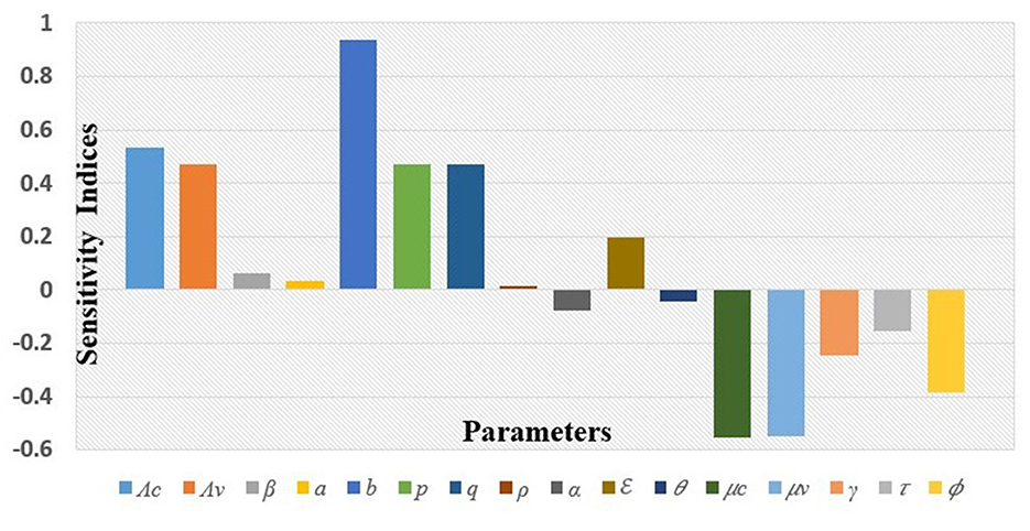
Figure 3. Graphical representation of the sensitivity indices of ℜ_c.

It can be read from the above index table in Table 2 and from Figure 3, that the most sensitive parameter is the fly's biting rate (b). Other parameters such as the spontaneous recovery rate (γ), rate of administration of antibiotics (τ), and rate of insecticide application (ϕ), among others, are also sensitive to the mastitis effective reproduction number, ℜ_c. To interpret these, ${\chi }_b^{{\Re }_c}=\mathrm{\text{+ 0}}\mathrm{\text{.9367111925}}$ implies that increasing (or decreasing) b by 10% increases (or decreases) ℜ_c by 9.367%; while ${\chi }_{\varphi }^{{\Re }_c}=-\mathrm{\text{0}}\mathrm{\text{.3857046086}}$ means that increasing (or decreasing) ϕ by 10% decreases (or increases) ℜ_c by 3.857%. The interpretation of the sensitivity indices of other parameters follows a similar manner as for b and ϕ.

4. Numerical simulations and discussion

This section presents the numerical simulation results for the mastitis model (3). The simulations were carried out with the aid of Maple 18.0 software to show the solution of the model equation, the global stability of the mastitis-free equilibrium, and the effects of sensitive parameters on mastitis transmission and control.

The parameter values used for the numerical simulations were sourced from existing literature, and where unavailable, values were assumed and fixed within a reasonable range as given in Table 1. The initial conditions are: S_c(0) = 500, E(0) = 100, A(0) = 30, I_c(0) = 50, C(0) = 20, R(0) = 10, for cattle population; and S_v(0) = 750, I_v(0) = 100, for fly population.

The results of the numerical simulations are given in Figures 4–11 to illustrate the system's behavior for different values of the mastitis model's parameters.

FIGURE 4

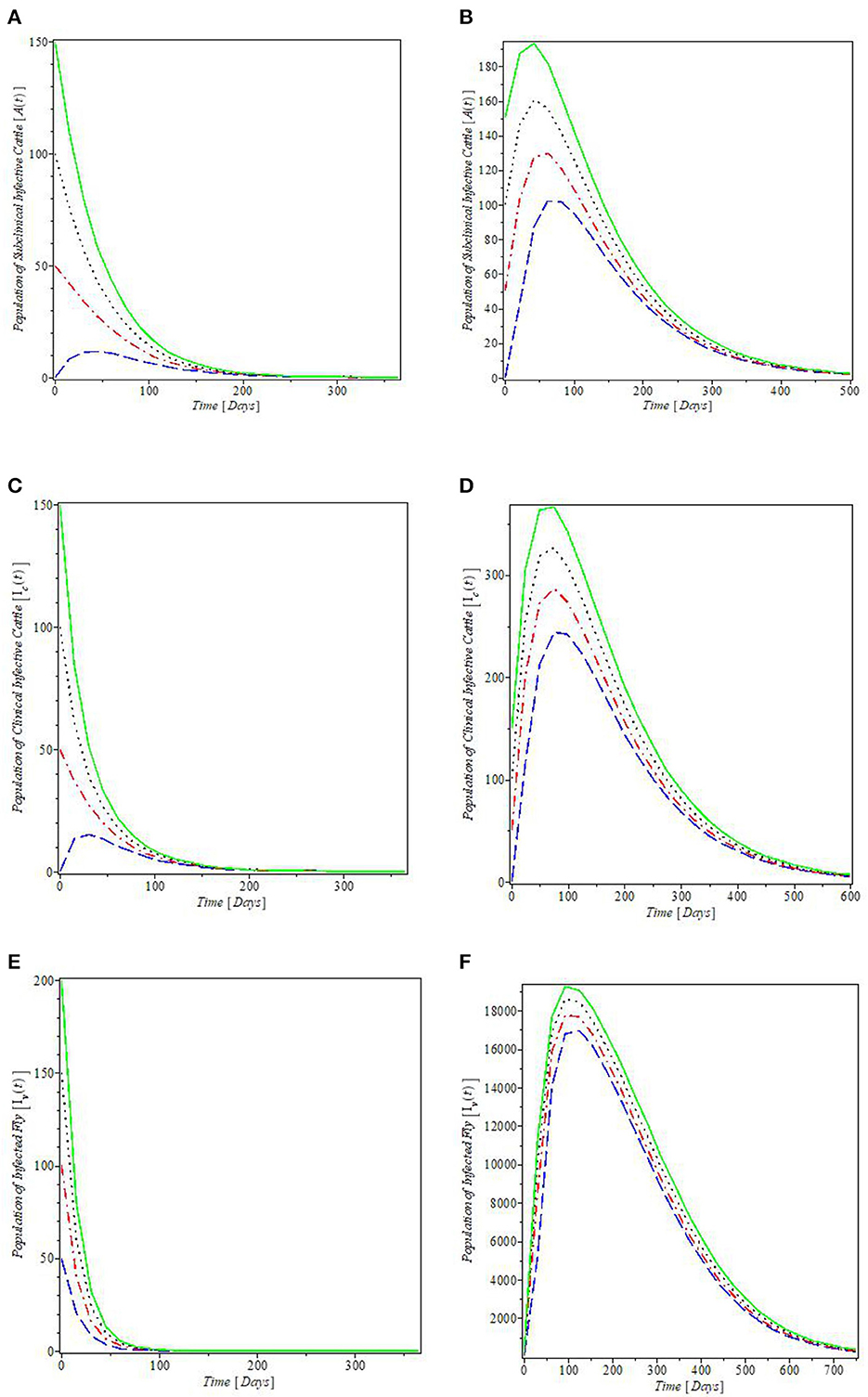
Figure 4. Plot of the global stability of the equilibria with various initial conditions: (A, C, E) are the global stability plots for the Mastitis-free equilibrium; (B, D, F) are the global stability plots for the Mastitis-endemic equilibrium.

The plots in Figure 4 illustrated the global stabilities of the mastitis-free and mastitis-endemic equilibria, E₀ and E_e, and they agree with the results of the global stability analyses given in Theorems 5 and 6. These results imply that regardless of the initial value of the infective, mastitis can be wiped out from both cattle and fly populations, whenever ℜ_c < 1, since the plots in Figures 4A, C, E revealed that the solutions converge at the mastitis-free equilibrium points for subclinical and clinical infective cattle population and infected fly population. It should be noted that this result may not hold for the cases where the mastitis-endemic equilibria co-exist with the mastitis-free equilibrium at ℜ_c < 1, because at this point, the mastitis model exhibits backward bifurcation as shown in Figure 2B. However, the reverse is the case when ℜ_c > 1, since the plots in Figures 4B, D, F showed that the infective populations converge at the endemic equilibrium above the x-axis.

Figure 5 is the plots of all the solutions for both populations against time for the given parameter values in Table 1. The plot in Figure 5A indicates that the susceptible cattle declines as a result of the infection. This consequently increases the population of exposed cattle. The recovered cattle population increases due to the presence of various control measures. In Figure 5B, the plot shows the behavior of the fly population with time. The plot revealed that both susceptible and infected flies increase with time and the susceptible later decreases just above 3,000 flies.

FIGURE 5

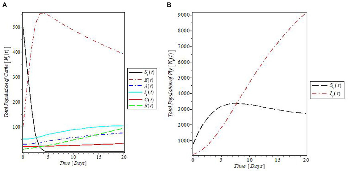
Figure 5. Plot of the (A) cattle and (B) fly populations with time at the given model's parameters.

The effects of the fly's biting rate (b) on the dynamics of mastitis disease were shown in Figures 6A–F. It was revealed by the plot in Figures 6A, E that increase in the fly's rate of biting (b) decreases the populations of the susceptible cattle and fly. This, in turn, caused an increase in the population of the subclinical infective, clinical infective, and chronic infective cattle, and the infected flies, as shown by the plots in Figures 6B–D, F, respectively. In Figure 7, the effects of the cattle transmission rate, β, were investigated. The plots in the Figure showed that an increase in the rate of transmission via contact with the infectious cattle declines the population of susceptible cattle, as can be seen in the plot in Figure 7A, while the increase in this rate caused an increase in the populations of the subclinical infective, clinical infective, and chronic infective cattle as depicted by the plots in Figures 7B–D, respectively.

FIGURE 6

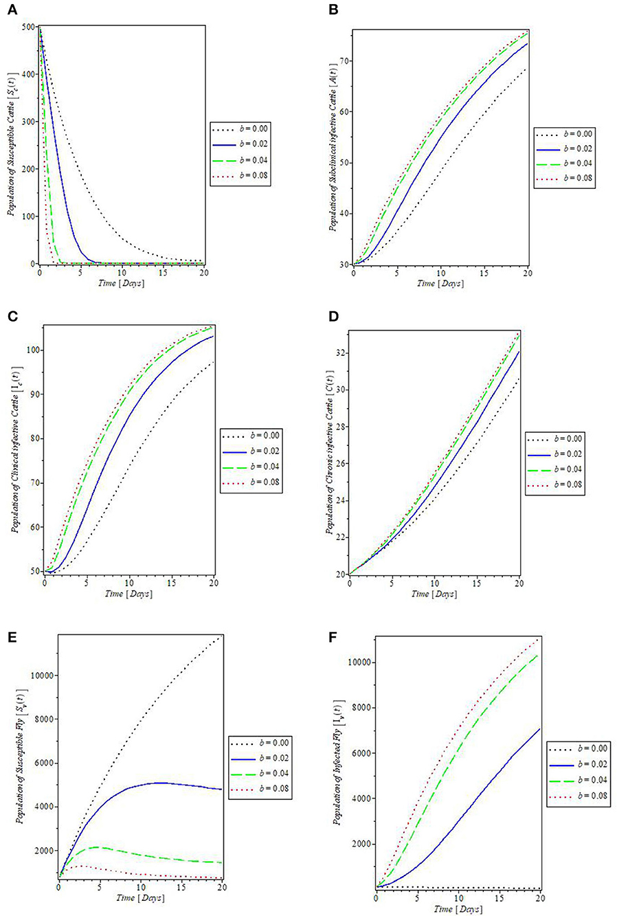
Figure 6. Plot of the effect of fly's biting rate “b” on the (A) susceptible cattle, (B) subclinical infective cattle, (C) clinical infective cattle, (D) chronic infective cattle, (E) susceptible fly, and (F) infected fly populations.

FIGURE 7

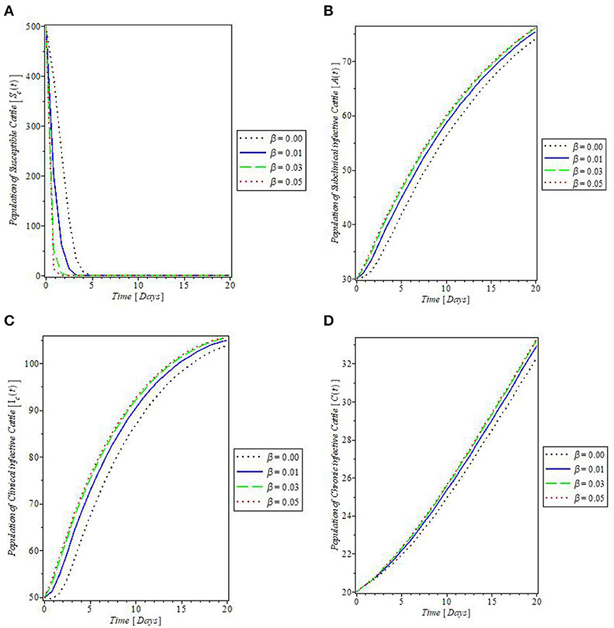
Figure 7. Plot of the effect of cattle's transmission rate “β” on the (A) susceptible cattle, (B) subclinical infective cattle, (C) clinical infective cattle, and (D) chronic infective cattle populations.

From Figure 8, which showed the effect of the rate of spontaneous recovery, γ, on the cattle populations, it was observed that an increased rate of spontaneous recovery, γ, significantly reduced the infectious cattle, including the chronic infective ones, as shown by the plots in Figures 8A–C. Consequent to this reduction, the recovered cattle population was increased. This is depicted by the plot in Figure 8D. Furthermore, we investigated the effect of boosting the recovery from mastitis disease via the administration of pharmaceutical/non-pharmaceutical therapy (such as the use of antibiotics), the rate of which is denoted by τ. It was then observed that the use of this control measure has a significant effect on decreasing mastitis disease, as can be seen from the plots in Figures 9A, B, that increase in τ decreased the populations of the clinical infective and chronic infective cattle but increased the population of the recovered cattle as in Figure 9C. This control measure also, interestingly, decreased the population of the infected flies, as shown in Figure 9D, thereby reducing the number of infected flies available to cause mastitis disease whenever biting occurs.

FIGURE 8

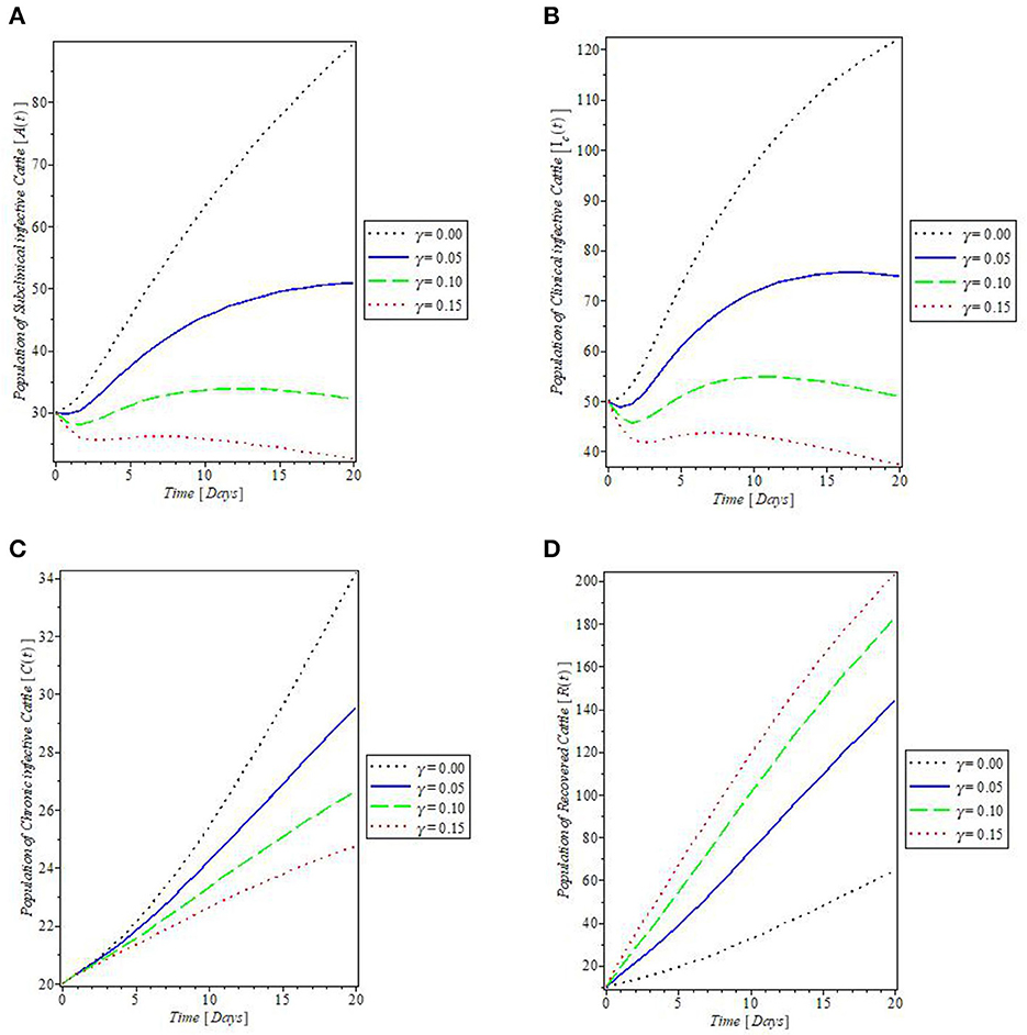
Figure 8. Plot of the effect of spontaneous recovery rate “γ” on the (A) subclinical infective cattle, (B) clinical infective cattle, (C) chronic infective cattle, and (D) recovered cattle populations.

FIGURE 9

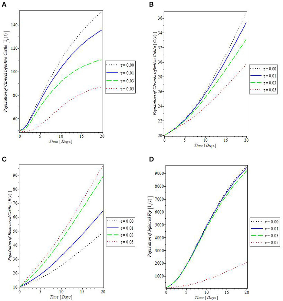
Figure 9. Plot of the effect of rate of antibiotics administration “τ” on the (A) clinical infective cattle, (B) chronic infective cattle, (C) recovered cattle, and (D) infected fly populations.

The plot in Figure 10 showed the effect of the rate of culling “τ” on the dynamics of mastitis disease. Culling is a control measure that involved the total separation of infected, and weak cattle from the herd, to prevent the further spread of the disease. The result of this control measure as shown in Figure 10 revealed that an increase in the rate of culling will decrease the population of the chronically infective cattle and so they do not partake in the transmission of mastitis disease. This is one of the assumptions on which the proposed mastitis model in this study is based.

FIGURE 10

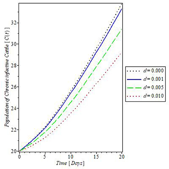
Figure 10. Plot of the effect of rate of culling “d” on the dynamics of mastitis disease.

This study also simulated the effect of the rate of application of insecticides “ϕ” on the populations of flies that transmit mastitis disease, and the results are plotted in Figure 11. These plots showed that the more the use of insecticides against such flies, the lesser the population of the flies, irrespective of their infection status. This implies that both susceptible and infected fly's populations are reduced whenever insecticides are applied as revealed by the plots in Figures 11A, B, respectively.

FIGURE 11

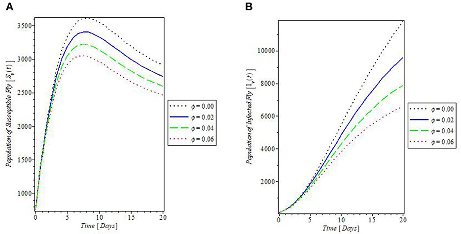
Figure 11. Plot of the effect of rate of application of insecticides “ϕ” on the (A) susceptible fly and (B) infected fly populations.

5. Conclusion

In this study, we proposed and formulated an epidemic mathematical model for the dynamics of mastitis disease in cattle (host) and fly (vector) populations with standard incidence rates. The intervention strategy focused on the treatment of infected cattle, culling of chronic infective cattle, and application of insecticides on the flies that bite cattle. The proposed model was shown to be epidemiologically feasible and mathematically well-posed by establishing that the solutions set is non-negative and bounded in a feasible region. The existence and stability of both disease-free and endemic equilibria were obtained, and these depended on the effective reproduction number, ℜ_c. If this threshold value, ℜ_c < 1, mastitis disease is under control, but if ℜ_c > 1, then mastitis will persist in the population.

We performed a sensitivity analysis on the effective reproduction number, ℜ_c, and the result revealed that the most sensitive parameter was the biting rate of flies. This can be significantly reduced by the use of insecticides, such as methoprene, synthetic pyrethroids, organophosphates, and abamectins [9] against the flies, as revealed by the results of the simulations. Other parameters such as the spontaneous recovery rate (γ), rate of administration of antibiotics (τ), and rate of insecticide application (ϕ), among others, are also sensitive to the mastitis effective reproduction number, ℜ_c. Therefore, mastitis control measures should be based on these parameters, among others, so that the spread of mastitis disease could be reduced in both cattle and fly populations.

The numerical simulations performed revealed that parameters like the biting rate of flies and cattle transmission rate both reduced healthy cows and increased mastitis infection in both populations. However, control measures such as infected cattle treatment (τ), culling of chronic infective cattle (d), and the use of insecticides against flies (ϕ), all have the effect of decreasing the spread of mastitis disease and decreasing the number of infective cattle and increasing healthy ones. It is, therefore, recommended that these control measures be adopted in the livestock and dairy industries, as this will increase the number of healthy cows available, and also improve the quantity and quality of milk produced for human consumption. Then meat and milk economy can also be greatly enhanced. Future study would be based on determining which of the control measures would yield an optimal result for controlling the disease. Control measures such as media advertisement and community awareness [36–38] would be explored, among others, in the optimal control analysis of the mastitis model.

Data availability statement

The original contributions presented in the study are included in the article/supplementary material, further inquiries can be directed to the corresponding author.

Author contributions

MA contributed to the conception of the study, model formulation of the study, methodology and analysis, numerical simulations, and write-up of sections of the manuscript. TO contributed to the model formulation of the study, methodology and analysis, and numerical simulations. Both authors contributed to the manuscript revision, read, and approved the final version of the submitted manuscript.

Acknowledgments

The authors are thankful to the editor and the reviewers for their comments and suggestions that helped in improving this study.

Conflict of interest

The authors declare that the research was conducted in the absence of any commercial or financial relationships that could be construed as a potential conflict of interest.

Publisher's note

All claims expressed in this article are solely those of the authors and do not necessarily represent those of their affiliated organizations, or those of the publisher, the editors and the reviewers. Any product that may be evaluated in this article, or claim that may be made by its manufacturer, is not guaranteed or endorsed by the publisher.

References

1. Kumar P, Ojasvita Deora A, Sharma H, Sharma S, Mittal D, Bhanot V, et al. Bovine mastitis: a review. Middle East J Sci Res. (2020) 28:497–507. doi: 10.5829/idosi.mejsr.2020.497.507

CrossRef Full Text

2. Tewari A. Bovine mastitis: an important diary cattle disease, technical report. Dairyman. (2014) 2014:62–5.

Google Scholar

3. National Mastitis Council (NMC). Current Concept of Bovine mastitis. 5th ed. Verona: National Mastitis Council (2011).

Google Scholar

4. Ruegg PL. A 100-year review: mastitis detection, management and prevention. J Diary Sci. (2017) 100:10381–97. doi: 10.3168/jds.2017-13023

PubMed Abstract | CrossRef Full Text | Google Scholar

5. Wattiaux MA. Mastitis: The Disease and its Transmission. Diary essentials, Babcock Institute for International Dairy Research and Development. Wisconsin: University of Wisconsin-Madison (2011).

6. Ruegg PL. New perspectives in udder health management. Vet Clin Food Anim. (2012) 28:149–63. doi: 10.1016/j.cvfa.2012.03.001

PubMed Abstract | CrossRef Full Text | Google Scholar

7. Arsenopoulos K, Triantafillous E, Filioussis G, Papadopoulos E. Fly repellency using deltamethrin may reduce intramammary infections of dairy cows under intensive management. Comp Immunol Microbiol Infect Dis. (2018) 61:16–23. doi: 10.1016/j.cimid.2018.11.001

PubMed Abstract | CrossRef Full Text | Google Scholar

8. Aligaz AA, Munganga JMW. Mathematical modelling of the transmission dynamics of contagious Bovine pleuropneumonia with vaccination and antibiotic treatment. J Appl Math. (2018) 2019:1–10. doi: 10.1155/2019/2490313

CrossRef Full Text | Google Scholar

9. Arnold M. Preventing Summer Mastitis in Heifers Begins with Horn Fly Control UK College of Agriculture, Food Environment, Cooperative Extension Service. (2019). Available online at: https://entomology.ca.uky.edu/files/recs0/ent12-dairy.pdf (accessed May 1, 2022).

10. Yeruham I, Braverman Y, Shipgel NY, Chizov-Ginzburg A, Saran A, Winkler M. Mastitis in dairy caused by Corynebacterium pseudotuberculosis and the feasibility of transmission by housefly I. Vet Quart. (1996) 18:87–9. doi: 10.1080/01652176.1996.9694623

PubMed Abstract | CrossRef Full Text | Google Scholar

11. Abdel-Rady A, Sayed M. Epidemiological studies on subclinical mastitis in dairy cows in assiut governorate. Veterinary World. (2009) 2:373–80. doi: 10.5455/vetworld.2009.373-380

PubMed Abstract | CrossRef Full Text

12. Rachah A, Dalen G, Norstebo H, Reksen O, Barlow JW. Deterministic modelling of the transmission dynamics of intramammary infections. J Phys Conf Ser. (2018) 1132:012053. doi: 10.1088/1742-6596/1132/1/012053

CrossRef Full Text | Google Scholar

13. Dalen G, Rachah A, Norstebo H, Schukken YH, Gröhn YT, Barlow JW, et al. Transmission dynamics of intramammary infections caused by corynebacterium species. J Dairy Sci. (2018) 101:472. doi: 10.3168/jds.2017-13162

PubMed Abstract | CrossRef Full Text | Google Scholar

14. Oltenacu PA, Natzke RP. Mathematical modelling of the mastitis infection process. J Dairy Sci. (1975) 15:515–21. doi: 10.3168/jds.S0022-0302(76)84233-6

PubMed Abstract | CrossRef Full Text | Google Scholar

15. Van-den-Driessche P, Watmough J. Reproduction number and sub-threshold endemic equilibria for computational models of diseases transmission. Math Biosci. (2002) 180:29–48. doi: 10.1016/s0025-5574(02)00108-6

PubMed Abstract | CrossRef Full Text | Google Scholar

16. Diekmann O, Heesterbeek JAP, Metz JAJ. On the definition and the computation of the basic reproduction ratio, Ro, in models for infectious diseases in heterogeneous populations. J Math Biol. (1990) 28:365. doi: 10.1007/BF00178324

PubMed Abstract | CrossRef Full Text | Google Scholar

17. Ouifki R, Banasia J. Epidemiological models with quadratic equation for endemic equilibrium – a bifurcation atlas. Math Model Appl Sci. (2020) 43:10413–29. doi: 10.1002/mma.6389

CrossRef Full Text | Google Scholar

18. Martcheva M. An Introduction to Mathematical Epidemiology. New York, NY: Springer (2015). doi: 10.1007/978-1-4899-7612-3

CrossRef Full Text | Google Scholar

19. Arino J, Milliken E. Bistability in deterministic and stochastic sliar-type models with imperfect and waning vaccine protection. J Math Biol. (2022) 84:61. doi: 10.1007/s00285-022-01765-9

PubMed Abstract | CrossRef Full Text | Google Scholar

20. Piazza N, Wang H. Bifurcation and sensitivity of immunity duration in an epidemic model. Int J Num Anal Modell Ser B. (2013) 4:179–202.

Google Scholar

21. Castillo-Chavez C, Song B. Dynamical models of tuberculosis and their applications. Math Biosci Eng. (2004) 1:361–404. doi: 10.3934/mbe.2004.1.361

PubMed Abstract | CrossRef Full Text | Google Scholar

22. Buonomo B, Lacitignola D. On the backward bifurcation of a vaccination model with nonlinear incidence. Nonlinear Anal Modell Control. (2011) 16:30–46. doi: 10.15388/NA.16.1.14113

CrossRef Full Text | Google Scholar

23. Madubueze CE, Kimbir AR, Aboiyar T. Global stability of ebola disease model with contact tracing and quarantine. Applic Appl Math Int J. (2018) 13:382–403.

Google Scholar

24. Bonyah E, Khan MA, Islam S. A theoretical Model for Zika Virus Transmission. PLoS ONE. (2017) 12:e0185540. doi: 10.1371/journal.pone.0185540

PubMed Abstract | CrossRef Full Text | Google Scholar

25. Castillo-Chavez C, Feng Z, Huang W. On the computation of R[[sb]]0[[/s]] and its role on global stability. Math Approach Emerg Reemerg Infect Dis Introd. (2002) 1:229–54. doi: 10.1007/978-1-4757-3667-0_13

CrossRef Full Text | Google Scholar

26. Adeyemi MO, Oluyo TO, Oladejo JK. Modelling the transmission and control dynamics of coronavirus disease with social distancing and contact tracing. Int J Innovat Sci Res Technol. (2020) 5:948–64.

PubMed Abstract | Google Scholar

27. Oladejo JK, Adeyemi MO, Oluyo TO. The impact of vaccine on the dynamical spread of Covid-19 pandemic. Int J Creat Res Thoughts. (2020) 8:4034–48.

Google Scholar

28. DeLeon CV. Construction of Lyapunov Functions for Classics SIS, SIR and SIRS Epidemic Model with Variable Population Size. Unite Academia de Mathematicas, Universidadn Autonoma de Guerrere, Mexico Facultad de Estudios Superiores Zarogoza, UNAM, Mexico (2009).

Google Scholar

29. Okuonghae D, Gumel AB, Ikhimwin BO, Iboi E. Mathematical assessment of the role of early latent infections and targeted control strategies of syphilis transmission dynamics. Acta Biotheor. (2018) 67:47–84. doi: 10.1007/s10441-018-9336-9

PubMed Abstract | CrossRef Full Text | Google Scholar

30. Obabiyi OS, Olaniyi S. Global stability analysis of malaria transmission dynamics with vigilant compartment. Electron J Differ Equ. (2019) 2019:1–10.

Google Scholar

31. Akanni JO, Akinpelu FO, Olaniyi S, Oladipo AT, Ogunsola AW. Modelling financial crime population dynamics: optimal control and cost-effectiveness analysis. Int J Dyn Control. (2019) 8:531–44. doi: 10.1007/s40435-019-00572-3

CrossRef Full Text | Google Scholar

32. LaSalle JP. The Stability of Dynamical systems, Regional conference Series in Applied Mathematics. Philadelphia, PA: SIAM (1976).

Google Scholar

33. Oluyo TO, Adeyemi MO. Sensitivity analysis of Zika epidemic model. Int J Sci Eng Res. (2018) 9:587–601.

34. Chitnis NR, Hyman JM, Chusing JM. Determining important parameters in the spread of malaria through the sensitivity analysis of a mathematical model. Bull Math Biol. (2008) 70:1272–96. doi: 10.1007/s11538-008-9299-0

PubMed Abstract | CrossRef Full Text | Google Scholar

35. Onuorah MO, Akinwande NI, Nasir MO, Ojo MS. Sensitivity analysis of lassa fever model. Int J Math Stat. (2016) 4:30–49.

Google Scholar

36. Ghosh I, Tiwari PK, Samanta S, Elmojtaba IM, Al-Salti N, Chattopadyay J. A simple SI-type model for HIV/AIDS with media and self-imposed psychological fear. Math Biosci. (2018) 306:160–9. doi: 10.1016/j.mbs.2018.09.014

PubMed Abstract | CrossRef Full Text | Google Scholar

37. Tiwari PK, Rai RK, Khajanchi S, Gupta RK, Misra AK. Dynamics of corona virus pandemic: effects of community awareness and global information campaigns. Eur Phys J Plus. (2021) 136:994. doi: 10.1140/epjp/s13360-021-01997-6

PubMed Abstract | CrossRef Full Text | Google Scholar

38. Rai RK, Khajanchi S, Tiwari PK, Venturino E, Misra AK. Impact of social media advertisement on the transmission dynamics of COVID-19 pandemic in India. J Appl Math Comput. (2022) 68:19–44. doi: 10.1007/s12190-021-01507-y

PubMed Abstract | CrossRef Full Text | Google Scholar