Bifurcation of solutions through a contact manifold in bidisperse models

1. Introduction

Polydisperse suspensions can be effectively modeled using balance equations that consider N continuous phases, where particles of species i with a volume fraction ϕ_i possess distinct properties such as size, density, and viscosity [1, 2]. A similar solution structure is applicable for modeling traffic and pedestrian flows as well [3, 4].

In the case of the bidisperse suspension model under consideration, the solution structure of the initial value problem for standard batch settling tests has been studied for situations where strict hyperbolicity is ensured [5], as well as when elliptic regions exist within the phase space [6]. This contribution focuses on the influence of a contact manifold within the phase space, which emerges under specific parameter settings. This contact manifold possesses the physical characteristic of coinciding particles settling velocities, which is of practical relevance since one common objective in the process control of solid-liquid separation processes is to minimize segregation effects [7]. At these optimal states, the phenomenon of solution bifurcation emerges.

The general form of kinematic sedimentation models for polydisperse suspensions consists of a system of N first-order hyperbolic equations. In this work, we consider a bidisperse suspension (N = 2) which exhibits a contact manifold capable of producing solution bifurcations. Specifically, the 2 × 2 system is given by:

$\begin{array}{ll}{\partial }_t{\varphi }_i+{\partial }_x{f}_i(\text{Φ})=0,f_i(\text{Φ})={\varphi }_i{v}_i(\text{Φ}),i=1,2,& (1)\end{array}$

where t represents time, x denotes depth, and the velocity components v_i(Φ) depend on the concentration vector $\text{Φ}={({\varphi }_1,{\varphi }_2)}^{\text{T}}$. The vector Φ represents the volume fractions of the solid phases and is constrained within the phase space of physically relevant concentrations

$\begin{array}{ll}{D}_{{\text{Φ}}^{\infty }}:=\{\text{Φ}={({\varphi }_1,{\varphi }_2)}^{\text{T}}\in {ℝ}^2|\begin{array}{l}{\varphi }_1,{\varphi }_2\ge 0,\hfill \\ \varphi :={\varphi }_1+{\varphi }_2\le {\varphi }^{\infty }\},\hfill \end{array}& (2)\end{array}$

where the total concentration ϕ: = ϕ₁ + ϕ₂ is upper-bounded by the maximum packing concentration ϕ^∞. The maximum packing manifold, denoted by

$\begin{array}{ll}{\partial }^{\infty }:=\{\text{Φ}={({\varphi }_1,{\varphi }_2)}^{\text{T}}|\varphi :={\varphi }_1+{\varphi }_2={\varphi }^{\infty }\},& (3)\end{array}$

represents the set of all maximal states.

The resulting system of conservation laws represents a mass balance for different solid species, where the non-linear flux function

$\begin{array}{l}f(\text{Φ}):={(f_1(\text{Φ}),f_2(\text{Φ}))}^{\text{T}}\end{array}$

can be derived from the corresponding momentum balances [1, 2, 8]. These components describe the flow process of dispersed solid phases within a liquid, considering the dispersed phases as a continuum.

The solid-fluid relative (“slip”) velocities

$\begin{array}{ll}{u}_i(\text{Φ}):=v_i(\text{Φ})-v_{\text{f}},& (4)\end{array}$

measure the absolute velocities v_i = v_i(Φ) relative to the fluid velocity v_f. The total volume displacement through horizontal sections is null:

$\begin{array}{l}(1-{\varphi }_1-{\varphi }_2)v_{\text{f}}(\text{Φ})+{\varphi }_1{v}_1(\text{Φ})+{\varphi }_2{v}_2(\text{Φ})=0.\end{array}$

By factoring out the slip velocities u_i, we can rewrite this mass balance equation as an equivalence, stating that if the solid volume is moving downward, then the fluid must move upward:

$\begin{array}{l}{v}_{\text{f}}(\text{Φ})+{\varphi }_1\left(v_1(\text{Φ})-v_{\text{f}}\right)+{\varphi }_2\left(v_2(\text{Φ})-v_{\text{f}}\right)=0\iff \\ v_{\text{f}}(\text{Φ})=-{\text{Φ}}^{\text{T}}\text{u}(\text{Φ})& (5)\end{array}$

The absolute velocities v_i = v_i(Φ) of representative solid particles depend on a linear combination of the relative velocities. This leads to the flux function with components

$\begin{array}{ll}{f}_i(\text{Φ})={\varphi }_i{v}_i(\text{Φ}),v_i(\text{Φ})=u_i(\text{Φ})-{\text{Φ}}^{\text{T}}u,i=1,2,& (6)\end{array}$

with $u={(u_1(\text{Φ}),u_2(\text{Φ}))}^{\text{T}}$. To close this flux function model, the slip velocities are further specified as

$\begin{array}{ll}{u}_i(\text{Φ})=v_{\infty i}{V}_i(\text{Φ}),& (7)\end{array}$

where v_∞i represents the Stokes velocity, quantifying the settling velocity of an individual particle in the fluid. Additionally, V_i(Φ) denotes the hindered-settling velocity, which is a non-increasing function of the components of Φ as discussed in [9]. Following Richardson and Zaki [10], the hindered-settling velocity is defined as

$\begin{array}{ll}{V}_i(\text{Φ}):=\{\begin{array}{ll}{(1-\varphi )}^{n_i-1}\hfill & \text{if 0}\le \varphi \le {\varphi }^{\infty },\hfill \\ 0\hfill & \text{otherwise,}\hfill \end{array}i=1,2,& (8)\end{array}$

where n_i > 1 accounts for the slowing down of the process at increasing concentrations. Combining assumptions (7) and (8) gives

$\begin{array}{ll}{u}_i(\text{Φ})=v_{\infty i}{(1-\varphi )}^{n_i-1}& (9)\end{array}$

for $\text{Φ}\in {\mathcal{D}}_{{\text{Φ}}^{\infty }}$.

Strictly hyperbolic systems of conservation laws, characterized by real and distinct eigenvalues of the Jacobian matrix of the flux function, provide a well-established framework for solving Riemann problems [11]. The system (1) with flux function (6) has been proven to be strictly hyperbolic for N = 2 in [2] and later extended to general N in [1]. However, these results are limited to hindered-settling factors that depend solely on the total concentration ϕ. It was previously believed that this strict hyperbolicity required constant exponents n₁ = n₂ = ⋯ = n_N, but [9] demonstrated that this restriction is unnecessary.

In [9], it was shown that strict hyperbolicity holds for general N≥2 and hindered-settling factors of the form V_i(Φ) = V_i(ϕ), as long as the inequality

$\begin{array}{ll}{u}_i^{\prime }(1-\varphi )-u_i<0& (10)\end{array}$

holds for all i = 1, …, N, where $u_i^{\prime }$ represents the derivative with respect to ϕ. In this case, the only requirement on the hindered-settling function V_i(Φ) = V_i(ϕ) is that it depends on the total concentration ϕ. The inequality (10) is satisfied when the relative velocities are ordered as u₁ > u₂ > ⋯ > u_n for any ϕ. For the hindered-settling function (8), this condition holds when the parameters are ordered as

$\begin{array}{ll}{v}_{\infty 1}>v_{\infty 2}>\cdots >v_{\infty N}\text{with\hspace{1em}}{n}_1<n_2<\cdots <n_N.& (11)\end{array}$

The strict hyperbolicity of the model can be verified using a secular equation framework introduced in [12] and adapted to size-dependent hindered-settling factors, not necessarily of the form (8), in [13]. This framework was further applied in [14] to analyze various hindered-settling functions.

Preliminary numerical simulations of Riemann problems for N = 3, with arbitrary parameter choices, indicate abrupt behavior when strict hyperbolicity fails, leading to the coincidence of eigenvalues. Across the contact manifold, there is a clear change in the solution structure with distinct bifurcations. Solutions of Riemann problems RP(0, Φ) for different Φ on opposite sides of the coincidence plane do not exhibit smooth transitions. However, when visualized in a 3D phase space, the assumed values traverse different planes and axes. The occurrence of this phenomenon of abrupt change, appearing even for N = 2, prompted our search for analytical insights, culminating in the present contribution.

This contribution focuses on the wave classification of 2 × 2 systems of conservation laws that arise as one-dimensional kinematic models for the sedimentation of bidisperse suspensions. Analyzing bidisperse suspensions provides insights into the flow properties of polydisperse suspensions, which are mixtures of small solid particles dispersed in a viscous fluid. Specifically, this study concentrates on the properties of the 2 × 2 system (1), flux function (6), and the closures (7) and (8). The model under consideration involves the following specifications in opposition to (11), that ensures the preservation of strict hyperbolicity:

(S1) v_∞1 > v_∞2 > 0,

(S2) n₁ > n₂ > 1,

(S3) ϕ^∞ ≡ 1.

For V_i(ϕ) given by (8), the flux function f(Φ) takes the form

$\begin{array}{l}{f}_1(\text{Φ})={\varphi }_1\left(v_{\infty 1}(1-{\varphi }_1){(1-\varphi )}^{n_1-1}-v_{\infty 2}{\varphi }_2{(1-\varphi )}^{n_2-1}\right),\\ f_2(\text{Φ})={\varphi }_2\left(v_{\infty 2}(1-{\varphi }_2){(1-\varphi )}^{n_2-1}-v_{\infty 1}{\varphi }_1{(1-\varphi )}^{n_1-1}\right),\end{array}$

for values $\text{Φ}\in {\mathcal{D}}_{{\text{Φ}}^{\infty }}$ and f₁(Φ) = f₂(Φ) = 0 otherwise. A special interest lies in the classification of the solution structure of the Riemann problem

$\begin{array}{ll}\text{Φ}(t=0,x)=\{\begin{array}{l}{\text{Φ}}^{-}\text{\hspace{1em}if\hspace{1em}}x<0,\hfill \\ {\text{Φ}}^{+}\text{\hspace{1em}if\hspace{1em}}x>0.\hfill \end{array}& (12)\end{array}$

For convenience, we refer to the Riemann problem consisting of the system of PDEs (1) with initial condition (12) as RP(Φ⁻, Φ⁺). Here, Φ⁻ and Φ⁺ denote the specified left and right values, respectively.

The model is applied to the batch settling process of an initially homogeneous suspension in a closed container, characterized by the initial-boundary value problem:

$\begin{array}{l}{\partial }_t{\varphi }_i+{\partial }_x{f}_i(\text{Φ})=0,i=1,2,\\ \text{Φ}(0,x)={\text{Φ}}_0(x),0\le x\le L,& (13)\end{array}$

$\begin{array}{ll}{f}_i(\text{Φ})=0,x\in \left\{0,L\right\},i=1,2,& (14)\end{array}$

here, L is the height of the domain, and the flux-density vector components are given by (6). Since the zero-flux boundary condition (14) holds, the initial-boundary data (13) and (14) can be replaced by the Cauchy data

$\begin{array}{ll}\text{Φ}(0,x)={\text{Φ}}_0(x)=\{\begin{array}{ll}O\hfill & \text{for x}<\text{0},\hfill \\ {\text{Φ}}_0\hfill & \text{for 0}\le \text{x}\le L,\hfill \\ {\text{Φ}}^{\infty }\hfill & \text{for x}>L,\hfill \end{array}& (15)\end{array}$

where O: = (0, 0)^T denotes the origin, and Φ^∞ represents a state on the maximum concentration manifold (3). Consequently, the Riemann problems RP(O, Φ₀) and $\text{RP}({\text{Φ}}_0,{\text{Φ}}^{\infty })$ are of particular interest.

This contribution offers analytical insights into the solution structure of the Riemann problem RP(O, Φ), which is of particular interest for describing the interactions at the upper interface between clear liquid and an initially homogeneous suspension during a batch settling process.

Previous studies have examined weakly hyperbolic systems, which are hyperbolic but not strictly hyperbolic, as models for multi-phase flow in porous media. For instance, the Corey model with convex permeability exhibits a single isolated point, known as the umbilic point, where strict hyperbolicity fails [15–19]. Another example of hyperbolicity loss occurs when the phase space contains an elliptic region, as observed in the case of the Stone model [20]. Coincidence along a curve can also lead to the loss of strict hyperbolicity, as shown in [21] for a 2 × 2 system.

To solve Riemann problems for weakly hyperbolic systems, the wave-curve method has been applied, which involves connecting a sequence of elementary waves. When strict hyperbolicity fails, the method of Liu for dealing with non-convex fluxes is not sufficient, and non-local branches of the Hugoniot locus must also be considered [22, 23]. The wave-curve method has been used in various contexts, such as the injection problem, which involves injecting a gas-water mixture into a porous medium containing oil [24], foam injection [25], and gravity effects [26].

For systems with a quadratic flux function, the solution in the vicinity of the umbilic point has been classified [18, 19, 27], and four distinct types of umbilic points associated with different shapes of nearby integral curves have been identified [19]. In the Corey model with convex permeability, only two types of umbilic points occur [18]. Based on this classification, certain types of Riemann problems have been considered in [16].

For non-strictly hyperbolic systems of two conservation laws that possess an umbilic point and an identity viscosity matrix, a systematic classification of solutions to the Riemann problem has been conducted [28, 29]. Non-classical waves and transitional shocks can arise due to a non-local Hugoniot locus, as shown in [30–32], and these transitional shocks are influenced by the regularization resulting from a non-identical viscosity matrix. It is worth noting that these types of shocks also occur on the same local branches.

Lastly, the concept of quasi-umbilic points has recently emerged in the context of porous media [26, 33]. it is briefly discussed in the Appendix (due to its only weak connection to RP(O, Φ), and in order to not divert the attention from the primary focus on solution construction and bifurcations).

2. Basic definitions

In this section, several definitions [26, 27, 34] are provided in order to facilitate the appropriate classification of the system under study.

Definition 1. The Hugoniot locus of a state Φ⁻, denoted as $\mathcal{H}({\text{Φ}}^{-})$, is the set of all states Φ⁺ that satisfy the Rankine-Hugoniot condition

$\begin{array}{ll}f({\text{Φ}}^{+})-f({\text{Φ}}^{-})=\sigma ({\text{Φ}}^{+}-{\text{Φ}}^{-}),& (16)\end{array}$

where σ = σ(Φ⁻, Φ⁺) is the propagation velocity of the discontinuity.

The shock classification according to Lax [35] is employed to refer to a subset of the Hugoniot locus that corresponds to a certain wave family. Admissible shocks within this classification are classified based on the magnitude of the shock speed with respect to the first and second eigenvalues on both sides of the discontinuity, as well as the speed of the discontinuity itself, see, e.g., [28, 35].

Definition 2. Three types of classical admissible shocks can be distinguished. The classification applies to a left state Φ⁻ and a right state Φ⁺ connected by the Rankine-Hugoniot condition (16) with a jump velocity σ = σ(Φ⁻, Φ⁺):

1-Lax shock: ${\text{λ}}_1({\text{Φ}}^{+})\le \sigma \le {\text{λ}}_1({\text{Φ}}^{-})$ and $\sigma \le {\text{λ}}_2({\text{Φ}}^{+})$,

2-Lax shock: ${\text{λ}}_2({\text{Φ}}^{+})<\sigma <{\text{λ}}_2({\text{Φ}}^{-})$ and ${\text{λ}}_1({\text{Φ}}^{-})\le \sigma$,

Over-compressive shock (OC): ${\text{λ}}_2({\text{Φ}}^{+})<\sigma <{\text{λ}}_1({\text{Φ}}^{-})$.

The definition of left- and right-characteristic shocks within this classification encompasses cases where the shock speed coincides with a characteristic speed (see Figure 1). While an over-compressible shock cannot be characteristic according to this definition, the limit of the aforementioned inequalities is included for 1-Lax shocks. On the other hand, for 2-Lax shocks, strict inequalities are required to avoid any ambiguities.

FIGURE 1

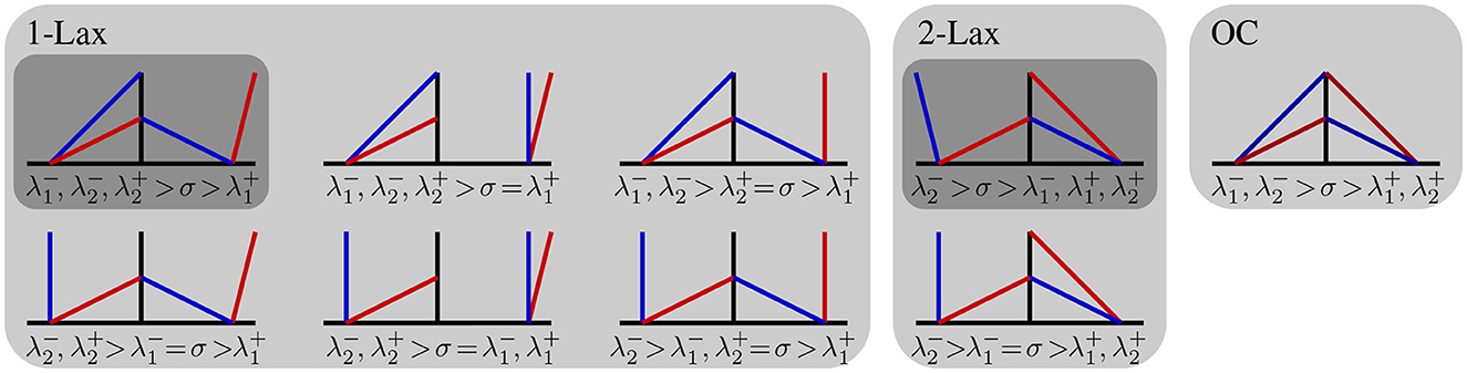
Figure 1. Schematic diagram of shock classification. Each type, as specified in Definition 2, is encompassed by cases shown with light shading. The cases corresponding to classic Lax classification are depicted with dark shading. The special case of shock velocity σ = 0 is included, where the classification relies on inequalities and equalities involving ${\text{λ}}_1^{-}={\text{λ}}_1({\text{Φ}}^{-})$, ${\text{λ}}_2^{-}={\text{λ}}_2({\text{Φ}}^{-})$, ${\text{λ}}_1^{+}={\text{λ}}_1({\text{Φ}}^{+})$, and ${\text{λ}}_2^{+}={\text{λ}}_2({\text{Φ}}^{+})$. The blue lines represent slow characteristic speeds, while the red lines represent fast characteristic speeds.

It is important to note that this extension deviates from the conventional approach presented in the seminal work of [28] or summarized in Table 1 of [36]. However, we have opted for this unconventional extension in order to maintain the continuity of the 1-Lax branch in the classification of the Hugoniot locus of the origin, as depicted in Figure 4 and established in Theorem 2. This choice facilitates a smoother and more coherent discussion in the subsequent analysis.

An inflection manifold ${\mathcal{I}}_i$ is determined for all states Φ where the i-th eigenvalue achieves either a maximum or minimum value along the integral curve of the same family.

Definition 3. The i-th inflection manifold is defined as

$\begin{array}{l}{I}_i:=\{\text{Φ}\in D_{{\text{Φ}}^{\infty }}|\text{∇}{\text{λ}}_i(\text{Φ})·r_i(\text{Φ})=0\},\end{array}$

where λ_i is the i-th eigenvalue of the Jacobian matrix of the flux function and r_i is the non-null corresponding eigenvector.

the invariant manifolds defined in [37], we introduce the following concept:

Definition 4. An i-th contact manifold occurs when the i-th integral curve passing through a state Φ^o coincides with a part of the Hugoniot locus $\mathcal{H}({\text{Φ}}^o)$, such that any state Φ on this intersection satisfies

${\text{λ}}_i({\text{Φ}}^o)=\sigma ({\text{Φ}}^o,\text{Φ})={\text{λ}}_i(\text{Φ}),$

for the shock speed σ(Φ^o, Φ).

A necessary condition for establishing an i-th contact manifold is that the integral curve is not a rarefaction in the usual sense, but rather that the characteristic speed remains fixed along the curve.

For states on a contact manifold the following transitivity rule holds: if Φ₁ and Φ₂ mutually belong to the Hugoniot locus of the other, connected by a shock of speed σ = σ(Φ₁, Φ₂), and if Φ₂ is on the Hugoniot locus of a state Φ₃ by a shock of the same speed σ, then Φ₁ belongs to $\mathcal{H}({\text{Φ}}_3)$ and σ(Φ₁, Φ₃) also coincides with σ. This fundamental property is known as the triple shock rule [15, 23, 34]. Another useful version of this rule is stated as follows.

Lemma 1. Let Φ₁, Φ₂, Φ₃ be non-collinear states such that Φ₁, Φ₂ belong to $\mathcal{H}({\text{Φ}}_3)$ and Φ₁ belongs to $\mathcal{H}({\text{Φ}}_2)$, then σ(Φ₁, Φ₂) = σ(Φ₂, Φ₃) = σ(Φ₁, Φ₃).

On a contact manifold, rarefactions and shocks are indistinguishable since all speeds align with a characteristic speed [37]. Remarkably, for the Hugoniot locus of the origin, the constant characteristic speed corresponds to a straight line and coincides with the integral curves.

3. Contact manifold

If the specifications (S1) and (S2) of the considered model hold, then it is possible to identify a contact manifold within the phase space. This manifold turns out to be decisive in characterizing solutions of Riemann problems, in particular because the origin is connected to this manifold by means of a right characteristic 1-Lax shock.

Definition 5. Given a state ${\text{Φ}}^{\star }=({{\varphi }^{\star }}_1,{{\varphi }^{\star }}_2)\in {\mathcal{D}}_{{\text{Φ}}^{\infty }}$, such that $v_1({\text{Φ}}^{\star })=v_2({\text{Φ}}^{\star })$, the following subset of phase space which contains Φ^⋆ is defined

$\begin{array}{ll}C({\text{Φ}}^{\star }):=\{\text{Φ}\in D_{{\text{Φ}}^{\infty }}:v_1(\text{Φ})=v_2(\text{Φ})=v_1({\text{Φ}}^{\star })\}.& (17)\end{array}$

The state Φ^⋆ serves as representative of the set $\mathcal{C}({\text{Φ}}^{\star })$. The definition of a set $\mathcal{C}({\text{Φ}}^{\star })$ unifies two complementary properties:

(1) v₁(Φ) = v₂(Φ) for all $\text{Φ}\in \mathcal{C}({\text{Φ}}^{\star })$,

(2) $v_i({\text{Φ}}^{-})=v_i({\text{Φ}}^{+})$ for ${\text{Φ}}^{-},{\text{Φ}}^{+}\in \mathcal{C}({\text{Φ}}^{\star })$ and i = 1, 2.

Property (1) denotes the local coincidence of velocities between different phases within a specific state, while property (2) describes the constancy of velocities within a single family along the manifold. Actually, a set $\mathcal{C}({\text{Φ}}^{\star })$ is a contact manifold for a broad class of flux functions that have a the considered structure. All the states belonging to this contact manifold share the same Hugoniot locus.

Lemma 2. If the flux function of the system (1) has the structure

$\begin{array}{ll}{f}_i(\text{Φ})={\varphi }_i{v}_i(\text{Φ}),& (18)\end{array}$

then any set $\mathcal{C}({\text{Φ}}^{\star })$ is a contact manifold with constant shock speed

$\begin{array}{ll}\sigma ({\text{Φ}}^{-},{\text{Φ}}^{+})=v_1({\text{Φ}}^{\star }).& (19)\end{array}$

Moreover, if the structure of the flux function (18) is such that the absolute velocity v depends only on the total concentration ϕ, namely

$\begin{array}{ll}{v}_i(\text{Φ})=v_i(\varphi ),& (20)\end{array}$

then the contact manifold $\mathcal{C}({\text{Φ}}^{\star })$ consists of the line

$\begin{array}{ll}C({\text{Φ}}^{\star })=\{\text{Φ}\in D_{{\text{Φ}}^{\infty }}:|{\varphi }_1+{\varphi }_2={\varphi }^{\star }\},& (21)\end{array}$

where ${\varphi }^{\star }={{\varphi }^{\star }}_1+{{\varphi }^{\star }}_2$ is the total concentration of Φ^⋆.

Proof. According to the definition in equation (17), any states ${\text{Φ}}^{-},{\text{Φ}}^{+}\in \mathcal{C}({\text{Φ}}^{\star })$ satisfy that

$v_1({\text{Φ}}^{-})=v_2({\text{Φ}}^{-})=v_1({\text{Φ}}^{+})=v_2({\text{Φ}}^{+})=v_1({\text{Φ}}^{\star }),$

such that one can factorize

$\begin{array}{ll}{\varphi }_i^{+}{v}_i({\text{Φ}}^{+})-{\varphi }_i^{-}{v}_i({\text{Φ}}^{-})=v_1({\text{Φ}}^{\star })({\varphi }_i^{+}-{\varphi }_i^{-}),i=1,2.& (22)\end{array}$

From the specific structure of the flux function (18) one recognizes that equation (22) states the Rankine-Hugoniot condition (16) with shock speed (19). Consequently, it is established that all states belonging to the set $\mathcal{C}({\text{Φ}}^{\star })$ mutually belong to the Hugoniot locus of each other. Furthermore, any two states within a set $\mathcal{C}({\text{Φ}}^{\star })$ can be connected by a shock of the same speed. Since shock speeds locally converge to an eigenvalue, on a manifold with constant shock speed any two states Φ⁻ and Φ⁺ have an eigenvalue that coincides with the shock speed,

$\begin{array}{l}{\text{λ}}_i({\text{Φ}}^{-})={\text{λ}}_i({\text{Φ}}^{+})=v_1({\text{Φ}}^{\star }).\end{array}$

This result confirms the definition of a contact manifold as stated in Definition 4. The line-shaped nature of the manifold $\mathcal{C}({\text{Φ}}^{\star })$ can be deduced from property (20), which ensures that the absolute velocities remain constant along the line in equation (21), that is, v₁(Φ) = v₂(Φ) for all $\text{Φ}\in \mathcal{C}({\text{Φ}}^{\star })$.

With this Lemma, nothing has been said yet about the existence of such a contact manifold for the considered model equation. Neither it is decided to which characteristic family the contact manifold belongs.

A further characterization of a set $\mathcal{C}({\text{Φ}}^{\star })$ is developed in the sequel, starting from properties that can be derived from the generic structure of the model, leading to properties that depend on particular model specifications. A property that can be used in several instances is

$\begin{array}{ll}{v}_1(\text{Φ})=v_2(\text{Φ})\iff u_1(\text{Φ})=u_2(\text{Φ}),& (23)\end{array}$

which holds directly from model setup (6) and the combined condition (9), together with $v_{\text{f}}(\text{Φ})=-{\text{Φ}}^{\text{T}}\text{u}$ [Here, property (23) takes the role of a generalized condition for (20)].

So far, we have shown that any set $\mathcal{C}({\text{Φ}}^{\star })$ is a contact manifold, which additionally takes the shape of a line. Moreover, under the considered model specifications, such manifolds effectively exist.

Lemma 3. If conditions (S1), (S2), and (S3) are satisfied, then two distinct contact manifolds exist in the domain ${\mathcal{D}}_{{\text{Φ}}^{\infty }}$, namely

$\begin{array}{ll}C({\text{Φ}}^{\text{x}}):=\{\text{Φ}={({\varphi }_1,{\varphi }_2)}^{\text{T}}|{\varphi }_1+{\varphi }_2={\varphi }^{\text{x}}\},& (24)\end{array}$

$\begin{array}{ll}C({\text{Φ}}^{\infty }):={\partial }^{\infty }=\{\text{Φ}={({\varphi }_1,{\varphi }_2)}^{\text{T}}|{\varphi }_1+{\varphi }_2={\varphi }^{\infty }\}.& (25)\end{array}$

The manifold $\mathcal{C}({\text{Φ}}^{\infty })$ is represented by any state Φ^∞ ∈ ∂^∞, that for handiness can be specified as Φ^∞ = (0, 1)^T. A representative state Φ^x that defines the contact manifold $\mathcal{C}({\text{Φ}}^{\text{x}})$ that is distinct to the manifold $\mathcal{C}({\text{Φ}}^{\infty })$ can be identified as

$\begin{array}{ll}{\text{Φ}}^{\text{x}}={({\varphi }^{\text{x}},0)}^{\text{T}},{\varphi }^{\text{x}}=1-{(v_{2\infty }/v_{1\infty })}^{1/(n_1-n_2)}.& (26)\end{array}$

In a geometrical interpretation, the plane $\mathcal{C}({\text{Φ}}^{\text{x}})$ corresponds to a crossing of speeds, and $\mathcal{C}({\text{Φ}}^{\infty })$ to a final encounter.

Proof. First, it is shown that the boundary ∂^∞ is a contact manifold. For any state Φ^∞ ∈ ∂^∞, if (S3) then one has $u_1({\text{Φ}}^{\infty })=u_2({\text{Φ}}^{\infty })=0$. By property (23) and since (5) holds, one obtains $v_1({\text{Φ}}^{\infty })=v_2({\text{Φ}}^{\infty })$ for any state Φ^∞ ∈ ∂^∞, satisfying the Definition (17) of the set $\mathcal{C}({\text{Φ}}^{\star })$, which, according to Lemma 2, is a contact manifold.

To show that there is an additional contact manifold $\mathcal{C}({\text{Φ}}^{\text{x}})$, it is necessary to find a set of states ${\text{Φ}}^{\text{x}}\notin \mathcal{C}({\text{Φ}}^{\infty })$ such that $v_1({\text{Φ}}^{\text{x}})=v_2({\text{Φ}}^{\text{x}})$. Because of property (23), this is equivalent to finding a Φ^x such that $u_1({\text{Φ}}^{\text{x}})=u_2({\text{Φ}}^{\text{x}})$. Solving

$\begin{array}{l}{v}_{1\infty }{(1-{\varphi }^{\text{x}})}^{n_1}=v_{2\infty }{(1-{\varphi }^{\text{x}})}^{n_2}\end{array}$

with respect to ϕ^x, which is the total concentration of any representative Φ^x, gives (26). The conditions (S1) and (S2) on the parameters guarantee the existence of ϕ^x ∈ (0, 1) (Actually, from (S2) is only used n₁ ≠ n₂).

Throughout this work, the notation $\mathcal{C}({\text{Φ}}^{\star })$ is used to refer to a generic contact manifold, whereas $\mathcal{C}({\text{Φ}}^{\text{x}})$ and $\mathcal{C}({\text{Φ}}^{\infty })$ refer to specific contact manifolds with assigned representative values Φ^x and Φ^∞, respectively. It turns out that there exists a peculiar Hugoniot locus in the model for the origin O as reference point. There are two local branches intersecting at the primary bifurcation given in O, these principal branches are the axes. However, the locus has four secondary bifurcation points with transverse lines (as non-local branches) joining them two by two in conjunction with these lines given by contact manifolds $\mathcal{C}({\text{Φ}}^{\text{x}})$ and $\mathcal{C}({\text{Φ}}^{\infty })$.

Lemma 4 (Hugoniot locus of origin). The Hugoniot locus $\mathcal{H}(O)$ of the origin O = (0, 0)^T consists of four branches: the two coordinate axes as local branches,

$\begin{array}{l}{\partial }^1:=\left\{\text{Φ}={(\varphi ,0)}^{\text{T}},\varphi \in \left[0,1\right]\right\},\\ {\partial }^2:=\left\{\text{Φ}={(0,\varphi )}^{\text{T}},\varphi \in \left[0,1\right]\right\},& (27)\end{array}$

with variable shock speed

$\begin{array}{ll}\sigma (O,\text{Φ})=v_i(\text{Φ})\text{for\hspace{1em}Φ}\in {\partial }^i,i=1,2,& (28)\end{array}$

and the two contact manifolds $\mathcal{C}({\text{Φ}}^{\text{x}})$ and $\mathcal{C}({\text{Φ}}^{\infty })$, identified by (25) and (24), as transversal branches with constant shock speed

$\begin{array}{ll}\sigma (O,\text{Φ})=v_1(\text{Φ})=v_2(\text{Φ})\text{for\hspace{1em}Φ}\in C({\text{Φ}}^{\star }).& (29)\end{array}$

Proof. With the structure of the flux function (6), the Rankine-Hugoniot condition (16) connecting the origin O with any state Φ takes the form

$\begin{array}{l}\sigma (O,\text{Φ}){\varphi }_i=v_i(\text{Φ}){\varphi }_i,i=1,2.\end{array}$

This system of two equations has two possible kinds of solution: On the local branches on the axes, ∂¹ and ∂², one of the two equations becomes obsolete, since both sides vanish on the considered axis. Therefore, the velocity of the remaining equation determines the shock speed as (28). On the transversal branches, $\mathcal{C}({\text{Φ}}^{\text{x}})$ and $\mathcal{C}({\text{Φ}}^{\infty })$, no such cancellation occurs. Therefore, for a solution to exist, the velocities must be equal, resulting in the speed (29).

The triple shock rule as stated in Lemma 1 applies to the connection of the origin to any state $\text{Φ}\in \mathcal{C}({\text{Φ}}^{\star })$ having speed (29) with any middle state Φ^M ∈ C(Φ^⋆) having speed (19). Indeed, O, Φ, Φ^M are not collinear, thus we have σ(O, Φ^M) = σ(Φ^M, Φ) = σ(O, Φ). This means that any (shock) solution O → Φ can be constructed by a first shock O → Φ^M followed by a second shock Φ^M → Φ of same speed; both solutions determine the same wave pattern, thus the same solution (This structural property plays a central role in the continuity of the bifurcation of solutions).

Another useful property is the convertibility of the relative velocity u_i(Φ) to the absolute velocity v_i(Φ) on the edges. A state Φ ∈ ∂ⁱ, i = 1, 2, on an axis has the representation Φ = ϕδ_i1e₁ + ϕδ_i2e₂, where e_k, k = 1, 2, are unit basis vectors and δ_ik is the Kronecker symbol. With this notation the definition of the relative velocity v_i(Φ) reduces to

$\begin{array}{ll}{v}_i(\text{Φ})=u_i(\text{Φ})-{\text{Φ}}^{\text{T}}u=u_i(\text{Φ})-\varphi u_i(\text{Φ})=(1-\varphi )u_i(\text{Φ}).& (30)\end{array}$

4. Characteristic speeds

System (1) can be written in quasi-linear form as

$\begin{array}{l}{\text{Φ}}_t+J(\text{Φ}){\text{Φ}}_x=0,\end{array}$

where RP(Φ) is the Jacobian matrix of the vector valued flux function $f(\text{Φ}):={(f_1(\text{Φ}),f_2(\text{Φ}))}^{\text{T}}$. The structure of the Jacobian matrix is examined for general N in [9, 14]; for our case it becomes

$\begin{array}{ll}J(\text{Φ})=\left(\begin{array}{cc}{J}_{11}(\text{Φ})& J_{12}(\text{Φ})\\ J_{21}(\text{Φ})& J_{22}(\text{Φ})\end{array}\right)=\left(\begin{array}{cc}{v}_1+u_{11}{\varphi }_1& u_{12}{\varphi }_1\\ u_{21}{\varphi }_2& v_2+u_{22}{\varphi }_2\end{array}\right),& (31)\end{array}$

or componentwise as

$\begin{array}{l}{J}_{ij}=v_i{\delta }_{ij}+{\varphi }_i{u}_{ij},i,j=1,2,\end{array}$

where δ_ij is the Kronecker symbol, v_i is the absolute velocity (4), and u_ij is specified as

$\begin{array}{ll}{u}_{ij}=u_{ij}(\text{Φ})=u_i^{\prime }(\text{Φ})-{\text{Φ}}^{\text{T}}{u}^{\prime }(\text{Φ})-u_j(\text{Φ}),i,j=1,2,& (32)\end{array}$

where $u^{\prime }(\text{Φ})=u_1^{\prime }(\text{Φ})u_2^{\prime }(\text{Φ}){}^{\text{T}}$. The short notation $u_i^{\prime }(\text{Φ})=v_{\infty i}{V}_i^{\prime }(\text{Φ}),i=1,2$ is used for the derivative of (7) [see, e.g., [9]], which, in a standard model like (9), acts as a derivative with respect to ϕ.

By definition a system is strictly hyperbolic if the Jacobian matrix of the flux function has distinct real eigenvalues. Thus, the system of conservation laws (1) is strictly hyperbolic if the discriminant

$\begin{array}{l}{\text{Δ}}_{\text{Φ}}:={\left(J_{11}(\text{Φ})-J_{22}(\text{Φ})\right)}^2+4J_{12}(\text{Φ})J_{21}(\text{Φ})\end{array}$

of the Jacobian matrix (31) is positive. For a hindered settling factor given by (8), strict hyperbolicity holds for identical exponents n₁ = n₂, see [2], which is proofed by showing algebraically that Δ_Φ > 0 for Φ in the interior of the phase space ${\mathcal{D}}_{{\text{Φ}}^{\infty }}$ under the specification (S3) with ϕ^∞ = 1. Moreover, strict hyperbolicity also holds for the case with different exponents n₁ ≠ n₂. This can be shown by a straightforward calculation [9], which yields the discriminant composed by a sum of a square and a positive term

$\begin{array}{l}{\text{Δ}}_{\text{Φ}}={\left[(n_1{\varphi }_1-1)u_1(\text{Φ})-(n_2{\varphi }_2-1)u_2(\text{Φ})\right]}^2\\ +4n_1{n}_2{\varphi }_1{\varphi }_2{u}_1(\text{Φ})u_2(\text{Φ}).& (33)\end{array}$

This term is positive because of conditions (S1) and (S2) together with the bounds ϕ₁, ϕ₂ > 0, ϕ = ϕ₁ + ϕ₂ < 1 (given by definition of the invariance domain ${\mathcal{D}}_{{\text{Φ}}^{\infty }}$) and the definition of u_i(Φ). The positivity of the discriminant Δ_Φ > 0 indicates strict hyperbolicity of the system (1).

The structure of the eigensystem of the Jacobian matrix RP of the flux function (6) is derived as outlined below. The eigenvalue calculation is tedious but straightforward, leading to the following result.

Lemma 5. The eigenvalues of the Jacobian matrix (31) are calculated as

$\begin{array}{l}\begin{array}{c}{\text{λ}}_{1,2}=\frac{1}{2}\left[v_1+v_2\right]-\frac{1}{2}\left[n_1{\varphi }_1{u}_1+n_2{\varphi }_2{u}_2\right]\pm \frac{1}{2}\sqrt{{\text{Δ}}_{\text{Φ}}},\end{array}\end{array}$

where Δ_Φ is the discriminant that takes the form (33).

With the help of this eigenvalue specification, the characterization of the contact manifold can be completed, which is formulated for any set $\mathcal{C}({\text{Φ}}^{\star })$, making it particularly applicable to the sets $\mathcal{C}({\text{Φ}}^{\text{x}})$ and $\mathcal{C}({\text{Φ}}^{\infty })$.

Theorem 1. The eigenvalues for any state $\text{Φ}\in \mathcal{C}({\text{Φ}}^{\star })$ can be specified as

$\begin{array}{ll}{\text{λ}}_1(\text{Φ})=v_1({\text{Φ}}^{\star })-\sqrt{{\text{Δ}}_{{\text{Φ}}^{\star }}}\text{and\hspace{1em}}{\text{λ}}_2(\text{Φ})=v_1({\text{Φ}}^{\star }).& (34)\end{array}$

Therefore, any set $\mathcal{C}({\text{Φ}}^{\star })$ is a contact manifold with respect to the second characteristic family.

Proof. Since any state Φ in the set $\mathcal{C}({\text{Φ}}^{\star })$ is characterized by definition by the property $v_1(\text{Φ})=v_2(\text{Φ})=v_1({\text{Φ}}^{\star })$, the eigenvalues become

$\begin{array}{l}{\text{λ}}_{1,2}(\text{Φ})=v_1({\text{Φ}}^{\star })-\frac{1}{2}\left[n_1{\varphi }_1{u}_1(\text{Φ})+n_2{\varphi }_2{u}_2(\text{Φ})\right]\pm \frac{1}{2}\sqrt{{\text{Δ}}_{\text{Φ}}}\\ =v_1({\text{Φ}}^{\star })-\frac{1}{2}\sqrt{{\text{Δ}}_{\text{Φ}}}\pm \frac{1}{2}\sqrt{{\text{Δ}}_{\text{Φ}}},\end{array}$

giving the pair of eigenvalues (34). Here, the last step is justified by property (23), i.e., the equivalence of the equalities v₁(Φ) = v₂(Φ) and u₁(Φ) = u₂(Φ). Specifically, one can relate the term within the brackets to the discriminant (33) as

$\begin{array}{l}{\left[n_1{\varphi }_1{u}_1+n_2{\varphi }_2{u}_2\right]}^2={\left[n_1{\varphi }_1{u}_1-n_2{\varphi }_2{u}_2\right]}^2+4n_1{n}_2{\varphi }_1{\varphi }_2{u}_1{u}_2\\ ={\text{Δ}}_{\text{Φ}},\end{array}$

which is valid in the special case when u₁(Φ) = u₂(Φ).

The association of the contact manifold with the second family can be seen from the fact that the eigenvalue λ₂, according to the established values in (34), is constant on $\mathcal{C}({\text{Φ}}^{\star })$, ${\text{λ}}_2(\text{Φ})\equiv v_1({\text{Φ}}^{\star })$ for all $\text{Φ}\in \mathcal{C}({\text{Φ}}^{\star })$. With the shock speed established in (19) in Lemma 2, for the connection of any two states on $\mathcal{C}({\text{Φ}}^{\star })$, one gets

$\begin{array}{l}{\text{λ}}_2({\text{Φ}}^{-})=\sigma ({\text{Φ}}^{-},{\text{Φ}}^{+})={\text{λ}}_2({\text{Φ}}^{+})\end{array}$

for all ${\text{Φ}}^{-},{\text{Φ}}^{+}\in \mathcal{C}({\text{Φ}}^{\star })$ establishing that $\mathcal{C}({\text{Φ}}^{\star })$ is a 2-th contact manifold.

Theorem 1 applies to both contact manifold $\mathcal{C}({\text{Φ}}^{\text{x}})$ and $\mathcal{C}({\text{Φ}}^{\infty })$. For the line $\mathcal{C}({\text{Φ}}^{\infty })$, the contact manifold is additionally characterized with respect to the first characteristic family.

For $\text{Φ}\in \mathcal{C}({\text{Φ}}^{\text{x}})$, the smaller eigenvalue λ₁ depends on the discriminant, while only the larger eigenvalue ${\text{λ}}_2(\text{Φ})\equiv v_1({\text{Φ}}^{\text{x}})$ is constant, Thus, a contact manifold $\mathcal{C}({\text{Φ}}^{\star })$ is an integral curve of the second family. On the maximum packing manifold for $\text{Φ}\in {\partial }^{\infty }=\mathcal{C}({\text{Φ}}^{\infty })$, where ϕ₁ + ϕ₂ = 1 holds, both eigenvalues vanish; λ₁(Φ) = λ₂(Φ) = 0.

Theorem 1 states explicit expressions for the eigenvalues on the contact manifold $\mathcal{C}({\text{Φ}}^{\text{x}})$ and $\mathcal{C}({\text{Φ}}^{\infty })$, which are part of the Hugoniot locus of the origin as identified in Lemma 4. The remaining eigenvalues along the Hugoniot locus of the origin can be directly evaluated from the general eigenvalues according to Lemma 5. A more comprehensive presentation of these findings can be found in [38].

For Φ on an edge ∂ⁱ, i = 1, 2, i.e., ϕ_i = 0 for some i = 1, 2, as specified in (27), the discriminant reduces to ${\text{Δ}}_{\text{Φ}}={\left[u_{3-i}(\text{Φ})(n_{3-i}{\varphi }_{3-i}-1)\right]}^2$, where the subindex 3−i becomes 2 on the axis ∂¹ and 1 on the axis ∂². A simple calculation shows that for Φ = (ϕ, 0)^T ∈ ∂¹, the eigenvalues are

$\begin{array}{l}{\text{λ}}_{1,2}(\text{Φ})=\frac{1}{2}\{[(1\mp 1)-(2+(1\mp 1)n_1)\varphi ]u_1(\text{Φ})+(1\pm 1)u_2(\text{Φ})\}\\ =\{\begin{array}{l}{u}_2(\text{Φ})-\varphi u_1(\text{Φ}),\hfill \\ (1-(1+n_1)\varphi )u_1(\text{Φ}),\hfill \end{array}\end{array}$

and for Φ = (0, ϕ)^T ∈ ∂² the eigenvalues are

$\begin{array}{l}{\text{λ}}_{1,2}(\text{Φ})=\frac{1}{2}\{(1\mp 1)u_1(\text{Φ})+[(1\pm 1)-(2+(1\pm 1)n_2)\varphi ]u_2(\text{Φ})\}\\ =\{\begin{array}{l}(1-(1+n_2)\varphi )u_2(\text{Φ}),\hfill \\ u_1(\text{Φ})-\varphi u_2(\text{Φ}).\hfill \end{array}\end{array}$

Within these eigenvalue characterizations we can distinguish the two types

$\begin{array}{ll}\{\begin{array}{ll}{\text{λ}}_a(\text{Φ}):=(1-(1+n_i)\varphi )u_i(\text{Φ}),\hfill & \text{\hspace{1em}for Φ}\in {\partial }_i,i=1,2,\hfill \\ {\text{λ}}_b(\text{Φ}):=u_{3-i}(\text{Φ})-\varphi u_i(\text{Φ}),\hfill & \text{\hspace{1em}for Φ}\in {\partial }_i,i=1,2.\hfill \end{array}& (35)\end{array}$

The notation λ_a(Φ), λ_b(Φ) with new subindices instead of λ₁(Φ), λ₂(Φ) is used since the order

$\begin{array}{ll}{\text{λ}}_a(\text{Φ})={\text{λ}}_1(\text{Φ})\le {\text{λ}}_2(\text{Φ})={\text{λ}}_b(\text{Φ})& (36)\end{array}$

cannot be always guaranteed. However, the notation λ₁, λ₂ is used whenever the order (36) can be assured, e.g., at the origin, where

$\begin{array}{l}{\text{λ}}_1(O)={\text{λ}}_a(O)=v_{\infty 2}<v_{\infty 1}={\text{λ}}_b(O)={\text{λ}}_2(O).\end{array}$

Generally, order changes can occur on both axes, as can be seen from Figure 3B. The order (36) holds only in the absence of such order changes [cf., [38]]. However, the occurrence of coincidence points does not affect the subsequent classification. In the sequel, it is shown how the eigenvalues λ_a(Φ) and λ_b(Φ) assume the role of the eigenvalue of the first or the second family in dependence of the value ϕ.

4.1. Inflection curves

The highly non-linear structure of the flux function makes it difficult –if not impossible– to obtain an explicit formula for inflection manifolds [27]. However, a characterization for states in the phase space can be obtained, since the inflection points there correspond to those of scalar equations. Namely, the eigenvalue λ_a(Φ) has the same form as the first derivative of the scalar flux function, whereas there is no correspondence for the additional eigenvalue λ_b(Φ), which emerges for the 2 × 2 system. The derivative

$\begin{array}{ll}{\text{λ}}_a^{\prime }(\varphi )=n_i\left((1+n_i)\varphi -2\right)u_i(\text{Φ})/(1-\varphi ),i=1,2& (37)\end{array}$

is well-defined for ϕ ∈ [0, 1). From (37) we have that ${\text{λ}}_a^{\prime }(\varphi )$ may vanish at ϕ = 1 and at ${\varphi }^{◇}=2/(1+n_i)$. The first case is of less significance because it represents a state at a vertex of the phase space. We have that ϕ^◇ ∈ (0, 1) since n_i is larger than one due to condition (S2). Thus, the state ϕ^◇ represents an inflection point and the states ${{\text{Φ}}^{◇}}_i$ such that ${\varphi }_i={\varphi }^{◇}$ and ϕ_j = 0 for i ≠ j ∈ {1, 2} belong to an inflection manifold (On edge ∂¹, there is a unique inflection point, see Lemma A1). The pertinence of the inflection points to the first characteristic family can be shown for general parameter settings.

Lemma 6. There is at least one inflection point located on each axis of the phase space ${\mathcal{D}}_{{\text{Φ}}^{\infty }}$, namely ${\text{Φ}}_1^{◇}:={(2/(1+n_1),0)}^T$ and ${\text{Φ}}_2^{◇}:={(0,2/(1+n_2))}^T$. Moreover, the corresponding eigenvalues belong to the first characteristic family.

Proof. The location of the inflection points on the axes is determined by finding the zeros of the corresponding eigenvalue derivatives (37).

The attribution of the inflection points to a certain characteristic family is done by comparing the magnitudes of the eigenvalues ${\text{λ}}_a({{\text{Φ}}^{◇}}_i)$ and ${\text{λ}}_b({{\text{Φ}}^{◇}}_i)$, both given by (35): Substituting ${\varphi }^{◇}=2/(1+n_i)$ one observes that

${\text{λ}}_a({{\text{Φ}}^{◇}}_i)+{\varphi }^{◇}{u}_i({{\text{Φ}}^{◇}}_i)=(1-n_i{\varphi }^{◇})u_i({{\text{Φ}}^{◇}}_i)=\frac{1-n_i}{1+n_i}{u}_i({{\text{Φ}}^{◇}}_i).$

Since u_i, u_j are non-negative and (1−n_i)/(1+n_i) is always negative by the parameter setting (S2), we have that

$\begin{array}{l}{\text{λ}}_a({{\text{Φ}}^{◇}}_i)<u_j({{\text{Φ}}^{◇}}_i)-{\varphi }^{◇}{u}_i({{\text{Φ}}^{◇}}_i)={\text{λ}}_b({{\text{Φ}}^{◇}}_i).\end{array}$

Therefore, in the inflection points on the axes, the eigenvalue λ_a corresponds to the first (smaller) eigenvalue λ₁ such that the eigenvalue order (36) holds.

The first inflection manifold, which has ${{\text{Φ}}^{◇}}_1$ and ${{\text{Φ}}^{◇}}_2$ as its endpoints, was numerically calculated and plotted in Figure 2A. Its location will be important for constructing the solution of RP(Φ, Φ^∞).

FIGURE 2

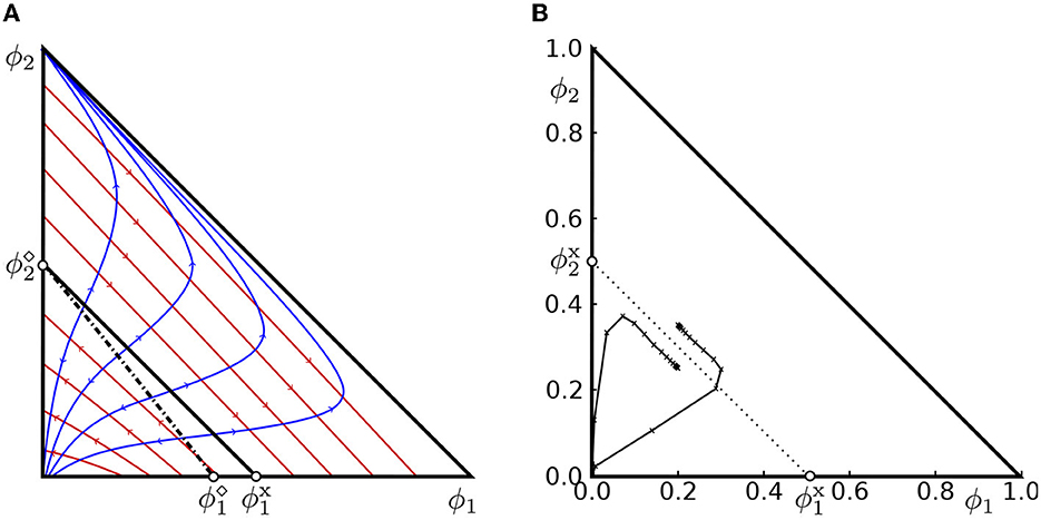
Figure 2. Phase space of Example 1 with parameters (44). (A) Integral curves in the ϕ₁ϕ₂−coordinate plane plotted as continuous curves. The arrows point into the direction of increasing eigenvalues. The first family (blue) crosses all lines with constant ϕ and the second family (red) connects the axes. Additionally, the contact manifold (solid dark curve) and the inflection manifold of the first family (dotted-dashed curve) are plotted. (B) Solution of Riemann problems RP[O,(0.2, 0.25)], RP[O,(0.2, 0.35)] using a finite difference method (low resolution).

4.2. Eigenvectors

The Jacobian matrix (31) with components (32) can be written as a rank two modification

$\begin{array}{ll}J=D+{\displaystyle \sum _{k=1}^2}{a}_k{b}_k^{\text{T}}=D+B{A}^{\text{T}}& (38)\end{array}$

of the diagonal matrix $D=\text{diag}(v_1,v_2)\in {ℝ}^{2\times 2}$, where one introduces column vectors a^k, b^k ∈ ℝ², k ∈ {1, 2}, in matrices

$\begin{array}{ll}A=\left(\begin{array}{cc}1& u_1+{\text{Φ}}^{\text{T}}{u}^{\prime }(\text{Φ})\\ 1& u_2+{\text{Φ}}^{\text{T}}{u}^{\prime }(\text{Φ})\end{array}\right)\text{and\hspace{1em}}B=\left(\begin{array}{cc}{\varphi }_1{u}_1^{\prime }(\text{Φ})& -{\varphi }_1\\ {\varphi }_2{u}_2^{\prime }(\text{Φ})& -{\varphi }_2\end{array}\right),& (39)\end{array}$

which both have rank two. The formula for the components of a right eigenvector can be deduced from secular equations and is given as a function of eigenvalues [14],

$\begin{array}{ll}\begin{array}{l}{r}_{ij}(\text{λ})=\frac{1}{v_j-\text{λ}}\left[b_j^1{\displaystyle \sum _{k=1}^2\frac{a_k^1{b}_k^2}{v_k-\text{λ}}}-b_j^2\left(1+{\displaystyle \sum _{k=1}^N}\frac{a_k^1{b}_k^1}{v_k-\text{λ}}\right)\right]\hfill \end{array},& (40)\end{array}$

where the parameters

$\begin{array}{ll}{a}_j^1=1,a_j^2=u_j(\text{Φ})+{\text{Φ}}^{\text{T}}{u}^{\prime },b_j^1={\varphi }_j{u}_j^{\prime },b_j^2=-{\varphi }_j,& (41)\end{array}$

correspond to the entries of the matrices A and B in (39). Whereas formula (40) holds for general rank two modifications of form (38), which are valid for systems of arbitrary size. By the abbreviation

$\begin{array}{l}{\text{Λ}}_j=\frac{{\varphi }_j}{v_j-\text{λ}},\end{array}$

one can rewrite the eigenvector (40) with parameters (41) compactly as

$\begin{array}{l}{r}_{*j}(\text{Φ},\text{λ}(\text{Φ}))={\text{Λ}}_j\left[1+{\displaystyle \sum _{k=1}^2}{\text{Λ}}_k(u_k^{\prime }-u_j^{\prime })\right],j=1,2,\end{array}$

with the components

$\begin{array}{l}{r}_{*1}={\text{Λ}}_1\left[1+{\text{Λ}}_2(u_2^{\prime }-u_1^{\prime })\right]=\frac{{\varphi }_2}{v_2-\text{λ}}+\frac{{\varphi }_1{\varphi }_2(u_1^{\prime }-u_2^{\prime })}{(v_1-\text{λ})(v_2-\text{λ})},\\ r_{*2}={\text{Λ}}_2\left[1+{\text{Λ}}_1(u_1^{\prime }-u_2^{\prime })\right]=\frac{{\varphi }_1}{v_1-\text{λ}}+\frac{{\varphi }_1{\varphi }_2(u_2^{\prime }-u_1^{\prime })}{(v_1-\text{λ})(v_2-\text{λ})}.\end{array}$

Multiplying by (v₁ − λ)(v₂ − λ), then the right eigenvectors get the form

$\begin{array}{ll}r(\text{Φ},{\text{λ}}_i(\text{Φ}))=\left(\begin{array}{c}{\varphi }_1(v_2(\text{Φ})-{\text{λ}}_i(\text{Φ}))+{\varphi }_1{\varphi }_2(u_2^{\prime }(\text{Φ})-u_1^{\prime }(\text{Φ}))\\ {\varphi }_2(v_1(\text{Φ})-{\text{λ}}_i(\text{Φ}))-{\varphi }_1{\varphi }_2(u_2^{\prime }(\text{Φ})-u_1^{\prime }(\text{Φ}))\end{array}\right),& (42)\end{array}$

for the corresponding eigenvalues λ_i(Φ), i = 1, 2.

Special eigenvectors, in particular those for the values of the Hugoniot locus of the origin, can be obtained from either exploiting the structure of the Jacobian matrix (31) or from using the analytical form of the eigenvectors (42). For instance, the eigenvectors on a set $\mathcal{C}({\text{Φ}}^{\star })$ that correspond to the second eigenvalue ${\text{λ}}_2({\text{Φ}}^{\star })=v_1({\text{Φ}}^{\star })$ have the form

$\begin{array}{ll}\begin{array}{l}{r}_2({\text{Φ}}^{\star })=\left(\begin{array}{c}1\\ -1\end{array}\right).\hfill \end{array}& (43)\end{array}$

In the origin one has $r_1(O)={(0,1)}^{\text{T}}$ and $r_2(O)={(1,0)}^{\text{T}}$.

4.3. Illustration of a benchmark example

For illustration, a benchmark example (Example 1) is considered with parameter setting

$\begin{array}{ll}{v}_{\infty 1}=1,v_{\infty 2}=1/2,and{n}_1=4,n_2=3,& (44)\end{array}$

that satisfies specifications (S1)–(S3). The integral curves in the ϕ₁ϕ₂−coordinate plane are shown in Figure 2A. The arrows point into the direction of increasing eigenvalues. The first characteristic family crosses all lines where ϕ is constant (except ϕ = 1) and the second family is connecting the axes. It can be recognized that the second family is genuinely non-linear out of Φ^x∪Φ^∞, whereas genuine non-linearity of the first family is lost at an inflection manifold, where the corresponding eigenvalues take their minimum.

The direction of increasing eigenvalues of the second characteristic family switches at the contact manifold. This direction switch impacts on the solution structure of the Riemann problem RP(O, Φ⁺), depending on the position of the right state Φ⁺ relative to the contact manifold, see Figure 2B for results of simulations by a finite difference method, namely a second-order central-upwind scheme where the numerical flux is a generalization of the Lax-Friedrichs flux, where the constant weight (Δt)/(2Δx) at the smoothing term is replaced by a locally adaptive weight, that take an upper estimate of the local velocities. Here we can observe that only a slight change of the Riemann data provokes a fundamental change of the solution path in the phase space.

5. Shock classification of Hugoniot locus of origin

In this Section the types of shocks that are connected to the origin are classified. The shock classification of Definition 2 distinguishes three different types of admissible shocks, namely 1-Lax, 2-Lax and overcompressive shocks. The locations of the shocks on the Hugoniot $\mathcal{H}(O)$ of the origin O = (0, 0)^T are identified in Lemma 4, which includes two contact manifolds. The shock classification builds on the eigenvalue analysis of Section 4 by comparing the shock speed and the eigenvalues in each state on the Hugoniot locus [see [38] for further graphical details].

A key feature in the determination of the shock type involves the switching of the order of the relative velocities at the threshold concentration ϕ^x,

$\begin{array}{ll}\{\begin{array}{l}{u}_1(\text{Φ})>u_2(\text{Φ})\text{\hspace{1em}for\hspace{1em}}\varphi \in [0,{\varphi }^{\text{x}}),\hfill \\ u_1(\text{Φ})=u_2(\text{Φ})\text{\hspace{1em}for\hspace{1em}}\varphi \in \{{\varphi }^{\text{x}},{\varphi }^{\infty }\},\hfill \\ u_1(\text{Φ})<u_2(\text{Φ})\text{\hspace{1em}for\hspace{1em}}\varphi \in ({\varphi }^{\text{x}},{\varphi }^{\infty }).\hfill \end{array}& (45)\end{array}$

This order switch is a direct consequence of the definition of the relative velocity (7), (8), together with the specifications (S1) and (S2).

A visual guide for the shock classification of shocks occurring between the origin and states located on the edges ∂¹ and ∂² is given in Figure 3, where the shock speeds are compared to the characteristic speeds. The shock classification is essentially obtained by speed comparisons. In the following result, the shock characterization is established for general parameter choices.

In Figure 3B, two important values appear:

(1) The threshold value ϕ^σ is defined as

$\begin{array}{ll}{\varphi }^{\sigma }=1{-}^{n_1}\sqrt{v_{\infty 2}/v_{\infty 1}}.& (46)\end{array}$

The value ϕ^σ characterizes a state Φ^σ = (^{ϕσ, 0)T} where $\sigma (O,{\text{Φ}}^{\sigma })={\text{λ}}_1(O)$;

(2) The value ϕ^u is defined as the unique zero root of

$\begin{array}{ll}(1-n_1\varphi ){(1-\varphi )}^{n_1-n_2}-v_{\infty 2}/v_{\infty 1}=0.& (47)\end{array}$

The value ϕ^u characterizes a state Φ^u = (^{ϕu, 0)T} where ${\text{λ}}_1({\text{Φ}}^u)={\text{λ}}_2({\text{Φ}}^u)$; a coincidence point over ∂¹-edge, a fact that is only proven in Lemma A1, which is of vital importance for the description of quasi-umbilic points.

FIGURE 3

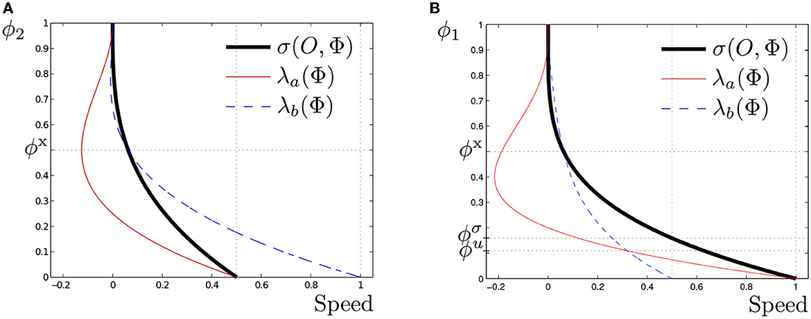
Figure 3. Eigenvalues and shock speeds of shocks from the origin to (A) the states Φ = (0, ϕ) ∈ ∂², ϕ ∈ [0, 1], (B) the states Φ = (ϕ, 0) ∈ ∂¹, ϕ ∈ [0, 1]. Bold solid curves represent the shock speed σ(O, Φ). The eigenvalues (characteristic speeds) given in (35) are represented as light solid curves for λ_a(Φ) and dashed curves for λ_b(Φ). The dotted horizontal lines represent heights corresponding to ϕ^x, ϕ^σ, and ϕ^u, ordered from top to bottom, the dotted vertical lines represent λ₁(O) and λ₂(O); hence the position of ϕ^σ.

Theorem 2. The Riemann problem

$\begin{array}{l}\text{RP}(O,\text{Φ}),\text{Φ}\in H(O)={\partial }^1\cup {\partial }^2\cup C({\text{Φ}}^{\text{x}})\cup C({\text{Φ}}^{\infty })\end{array}$

connecting the origin to a state of its Hugoniot locus is solved by a single shock of speed σ = σ(O, Φ), which can be classified according to Definition 2 as stated below.

Classification for $\underset{\_}{\text{Φ}={({\varphi }_1,0)}^{\text{T}}\in {\partial }^1}$:

$\begin{array}{ll}\text{2-Lax: }{\text{λ}}_{1,2}(\text{Φ})\le \sigma <{\text{λ}}_2(O)\text{ and }{\text{λ}}_1(O)<\sigma & \text{for }{\varphi }_1\in (0,{\varphi }^{\sigma }),\\ {\text{λ}}_{1,2}(\text{Φ})\le \sigma <{\text{λ}}_2(O)\text{ and }{\text{λ}}_1(O)=\sigma & \text{for }{\varphi }_1={\varphi }^{\sigma }.\\ \text{ OC: }{\text{λ}}_{1,2}(\text{Φ})<\sigma <{\text{λ}}_{1,2}(O)& \text{for }{\varphi }_1\in ({\varphi }^{\sigma },{\varphi }^{\text{x}}).\\ \text{1-Lax: }{\text{λ}}_1(\text{Φ})<\sigma <{\text{λ}}_{1,2}(O)\text{ and }\sigma ={\text{λ}}_2(\text{Φ})& \text{for }{\varphi }_1\in \left\{{\varphi }^{\text{x}},{\varphi }^{\infty }\right\},\\ {\text{ λ}}_1(\text{Φ})<\sigma <{\text{λ}}_{1,2}(O)\text{ and }\sigma <{\text{λ}}_2(\text{Φ})& \text{for }{\varphi }_1\in ({\varphi }^{\text{x}},{\varphi }^{\infty }).& (48)\end{array}$

The threshold value ϕ^σ given by (46).

Classification for $\underset{\_}{\text{Φ}={(0,{\varphi }_2)}^{\text{T}}\in {\partial }^2}$:

$\begin{array}{ll}\text{1-Lax: }{\text{λ}}_1(\text{Φ})<\sigma <{\text{λ}}_{1,2}(O)\text{ and }\sigma <{\text{λ}}_2(\text{Φ})& \text{for }{\varphi }_2\in (0,{\varphi }^{\text{x}}),\\ {\text{ λ}}_1(\text{Φ})<\sigma <{\text{λ}}_{1,2}(O)\text{ and }\sigma ={\text{λ}}_2(\text{Φ})& \text{for }{\varphi }_2\in \left\{{\varphi }^{\text{x}},{\varphi }^{\infty }\right\}.\\ \text{ OC: }{\text{λ}}_{1,2}(\text{Φ})<\sigma <{\text{λ}}_{1,2}(O)& \text{for }{\varphi }_2\in ({\varphi }^{\text{x}},{\varphi }^{\infty }).& (49)\end{array}$

Classification for $\underset{\_}{\text{Φ}\in \mathcal{C}({\text{Φ}}^{\text{x}})}$:

$\begin{array}{ll}\begin{array}{cc}\text{1-Lax:}& {\text{λ}}_1(\text{Φ})<\sigma <{\text{λ}}_{1,2}(O)\text{ and }\sigma ={\text{λ}}_2(\text{Φ}).\end{array}& (50)\end{array}$

Classification for $\underset{\_}{\text{Φ}\in \mathcal{C}({\text{Φ}}^{\infty })}$:

$\begin{array}{ll}\begin{array}{cc}\text{1-Lax:}& {\text{λ}}_1(\text{Φ})=\sigma <{\text{λ}}_{1,2}(O)\text{ and }\sigma ={\text{λ}}_2(\text{Φ}).\end{array}& (51)\end{array}$

Strict inequalities in the shock type classification (48)–(51) mean that the corresponding shocks are not characteristic shocks. For instance, for Φ ∈ ∂¹ there are no 1-Lax shocks that are characteristic at the left datum O.

Proof. The proof is done in two main steps:

1.- The first step is to relate the characteristic speeds λ_{1, 2}(O) and λ_{a, b}(Φ) to the shock speed σ(O, Φ) depending on the position of Φ.

2.- The second step consists in determining which shock classification applies according to Definition 2.

Table 1 provides an overview on the speed magnitudes for right states on the axes ∂¹ and ∂².

TABLE 1

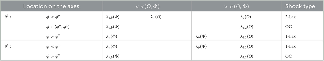
Table 1. Shock classification on Hugoniot locus of origin for states on the axes ∂¹ and ∂².

λ₂(O) compared to σ(O, Φ) on ∂¹ and ∂²

On the axes Φ ∈ ∂ⁱ\O the shock speed is limited as

$\begin{array}{ll}\begin{array}{l}\sigma (O,\text{Φ})=v_i(\text{Φ})<v_{\infty i}=\{\begin{array}{ll}{v}_{\infty 1}={\text{λ}}_2(O),\hfill & \text{\hspace{1em}if\hspace{1em}}i=1,\hfill \\ v_{\infty 2}={\text{λ}}_1(O)<{\text{λ}}_2(O),\hfill & \text{\hspace{1em}if\hspace{1em}}i=2,\hfill \end{array}\hfill \end{array}& (52)\end{array}$

since the shock speed

$\begin{array}{l}\sigma (O,\text{Φ})=v_i(\text{Φ})=(1-{\varphi }_i)u_i(\text{Φ})=v_{\infty i}{(1-{\varphi }_i)}^{n_i},i=1,2,\end{array}$

is monotonically decreasing on both axes ∂¹ and ∂² [Note that (52) excludes 2-Lax shocks on edge ∂²].

λ_a(Φ) compared to σ(O, Φ) on ∂¹ and ∂²

The eigenvalue λ_a(Φ) as specified in (35) leads to common properties for both axes. For all points Φ ∈ ∂ⁱ\O, i ∈ {1, 2}, along the axes one has

$\begin{array}{l}{\text{λ}}_a(\text{Φ})=[1-(1+n_i){\varphi }_i]u_i(\text{Φ})\\ <(1-{\varphi }_i)u_i(\text{Φ})=v_i(\text{Φ})=\sigma (O,\text{Φ}),i=1,2,& (53)\end{array}$

due to properties that apply on the axes, namely, the speed convertibility (30) and the shock speed (28).

λ_b(Φ) compared to σ(O, Φ) on ∂¹ and ∂²

The composition of the eigenvalue λ_b(Φ) depends on the inequality (45) between the relative velocities u₁(Φ) and u₂(Φ), and induces quite different behaviors on the edges. On the axis ∂¹ the eigenvalue λ_b(Φ) behaves as

$\begin{array}{ll}\begin{array}{l}\{\begin{array}{l}{\text{λ}}_b(\text{Φ})<\sigma (O,\text{Φ})\text{\hspace{1em}for\hspace{1em}}{\varphi }_1\in (0,{\varphi }^{\text{x}}),\hfill \\ {\text{λ}}_b(\text{Φ})=\sigma (O,\text{Φ})\text{\hspace{1em}for\hspace{1em}}{\varphi }_1\in \{{\varphi }^{\text{x}},{\varphi }^{\infty }\},\hfill \\ {\text{λ}}_b(\text{Φ})>\sigma (O,\text{Φ})\text{\hspace{1em}for\hspace{1em}}{\varphi }_1\in ({\varphi }^{\text{x}},{\varphi }^{\infty }),\hfill \end{array}\hfill \end{array}& (54)\end{array}$

because on ∂¹, the inequalities (45) between u₁(Φ) and u₂(Φ) implies that for the interval ${\varphi }_1\in [0,{\varphi }^{\text{x}})$ the eigenvalue (35) satisfies

$\begin{array}{l}{\text{λ}}_b(\text{Φ})=u_2(\text{Φ})-{\varphi }_1{u}_1(\text{Φ})<(1-{\varphi }_1)u_1(\text{Φ})=\sigma (O,\text{Φ}),\end{array}$

and for the other interval, where ${\varphi }_1\in ({\varphi }^{\text{x}},{\varphi }^{\infty }]$, the inequality switches sign.

On the axis ∂² one has

$\begin{array}{ll}\begin{array}{l}\{\begin{array}{l}{\text{λ}}_b(\text{Φ})>\sigma (O,\text{Φ})\text{\hspace{1em}for\hspace{1em}}{\varphi }_2\in [0,{\varphi }^{\text{x}}),\hfill \\ {\text{λ}}_b(\text{Φ})=\sigma (O,\text{Φ})\text{\hspace{1em}for\hspace{1em}}{\varphi }_2\in \{{\varphi }^{\text{x}},{\varphi }^{\infty }\},\hfill \\ {\text{λ}}_b(\text{Φ})<\sigma (O,\text{Φ})\text{\hspace{1em}for\hspace{1em}}{\varphi }_2\in ({\varphi }^{\text{x}},{\varphi }^{\infty }),\hfill \end{array}\hfill \end{array}& (55)\end{array}$

since, from the inequalities (45) for ${\varphi }_2\in [0,{\varphi }^{\text{x}})$, one obtains

$\begin{array}{l}{\text{λ}}_b(\text{Φ})=u_1(\text{Φ})-{\varphi }_2{u}_2(\text{Φ})>(1-{\varphi }_2)u_2(\text{Φ})=\sigma (O,\text{Φ})\end{array}$

and for ϕ ∈ (ϕ^x, ϕ^∞] the inequality switches sign.

On the edge ∂² the value of λ_b(Φ) determines whether the shock is 1-Lax or over-compressive. The shock type is decided by the relative magnitudes of u₁(Φ) contra u₂(Φ): The equality u₁(Φ) = u₂(Φ) only holds for ${\varphi }_2={\varphi }^{\text{x}}$ (and ${\varphi }_2={\varphi }^{\infty }$). On edge ∂¹ there is a coincidence of eigenvalues, see also Lemma A1.

λ₁(O) compared to σ(O, Φ) on ∂¹ and ∂²

Note that, along both axes σ(O, Φ) is a monotonically decreasing function with σ(O, Φ^∞) = 0. By (52) it is assured that σ(O, Φ) < λ₁(O) holds for all states on the axis ∂²\O. However, this does not hold for all states on the axis ∂¹\O.

Since $\underset{\epsilon \to 0}{lim}\sigma (O,(\epsilon ,0))={\text{λ}}_2(O)>{\text{λ}}_1(O)>0$ on the axis ∂¹, there exists a state Φ^σ = (^{ϕσ, 0)T} such that $\sigma (O,{\text{Φ}}^{\sigma })={\text{λ}}_1(O)$. In this state Φ^σ the equality

$\begin{array}{l}\sigma (O,{\text{Φ}}^{\sigma })=v_1({\text{Φ}}^{\sigma })=v_{\infty 1}{(1-{\varphi }_{\sigma })}^{n_1}=v_{\infty 2}={\text{λ}}_1(O)\end{array}$

holds, from which the characterization of ϕ^σ by (46) can be deduced. The shock speed σ(O, Φ) relates to λ₁(O) in dependence of ϕ^σ as

$\begin{array}{ll}\begin{array}{l}\{\begin{array}{l}\sigma (O,\text{Φ})>{\text{λ}}_1(O)\text{\hspace{1em}for\hspace{1em}}{\varphi }_1\in [0,{\varphi }^{\sigma }),\hfill \\ \sigma (O,\text{Φ})={\text{λ}}_1(O)\text{\hspace{1em}for\hspace{1em}}{\varphi }_1={\varphi }^{\sigma },\hfill \\ \sigma (O,\text{Φ})<{\text{λ}}_1(O)\text{\hspace{1em}for\hspace{1em}}{\varphi }_1\in ({\varphi }^{\sigma },{\varphi }^{\infty }].\hfill \end{array}\hfill \end{array}& (56)\end{array}$

Combining the previously established (52), (53), and (54), with the discrimination (56) implies that, on the axis ∂¹, for ϕ < ϕ^σ there is a 2-Lax shock, whereas for ϕ^σ < ϕ < ϕ^x the shock is over-compressive.

According to (53) and (54), there is a clear separation between the shock speeds for ϕ ∈ (ϕ^x, ϕ^∞) on the axis ∂¹:

$\begin{array}{ll}{\text{λ}}_1(\text{Φ})={\text{λ}}_a(\text{Φ})<\sigma (O,\text{Φ})<{\text{λ}}_b(\text{Φ})={\text{λ}}_2(\text{Φ}).& (57)\end{array}$

This separation allows an association of the eigenvalues according to (36). Similarly, according to (53) and (55), there is a clear separation between the shock speeds (57) for ϕ ∈ (0, ϕ^x) on ∂², which establishes the order of the eigenvalues as (36). For ϕ ∈ (ϕ^x, ϕ^∞) there is no clear eigenvalue separation, which however does not affect the fact that the shock is over-compressive.

Now we are able to conclude the shock classification on the axes: Putting the inequalities (52), (53), (55) together gives the shock classification (49) for right states on the axis ∂². Putting the inequalities (52), (53), (54), (56) together gives the shock classification (48) for right states on the axis ∂¹. See the resume in Table 1.

Contact manifold $\underset{\_}{\mathcal{C}({\text{Φ}}^{\text{x}})}$

The shock classification for states on the contact manifold $\text{Φ}\in \mathcal{C}({\text{Φ}}^{\text{x}})$ assures that all states are connected to the origin by a 1-Lax shock: Since the functions v₁(Φ) and v₂(Φ) take their maximum in the origin O and the origin is not part of the contact manifold, one has the strict inequality

$\begin{array}{ll}\sigma (O,\text{Φ})=v_1({\text{Φ}}^{\text{x}})<v_{\infty 1}={\text{λ}}_1(O)<v_{\infty 2}={\text{λ}}_2(O).& (58)\end{array}$

By the eigenvalue characterization (34) for states on $\mathcal{C}({\text{Φ}}^{\text{x}})$, and noting that Δ_Φ > 0 for all $\text{Φ}\in \mathcal{C}({\text{Φ}}^{\text{x}})$, one gets

$\begin{array}{ll}{\text{λ}}_1(\text{Φ})<\sigma (O,\text{Φ})=v_1(\text{Φ})={\text{λ}}_2(\text{Φ})& (59)\end{array}$

for all $\text{Φ}\in \mathcal{C}({\text{Φ}}^{\text{x}})$. The properties (58) and (59) are summarized in the shock classification (50).

Contact manifold $\underset{\_}{{\partial }^{\infty }=\mathcal{C}({\text{Φ}}^{\infty })}$

For states on the maximum packing manifold Φ ∈ ∂^∞ one has vanishing eigenvalues,

$\begin{array}{l}0={\text{λ}}_1(\text{Φ})={\text{λ}}_2(\text{Φ})=\sigma (O,\text{Φ})<{\text{λ}}_1(O)<{\text{λ}}_2(O),\end{array}$

which leads to classification (51).

Figure 4 displays the different shock types for states connected with the origin, as elaborated in Theorem 2. The 1-Lax states of $\mathcal{H}(O)$ are shown as blue dashed lines. States on the contact manifold $\mathcal{C}({\text{Φ}}^{\text{x}})$ satisfy the 1-Lax conditions being characteristic in the second family at the right state. Similarly, the states on the maximum packing $\mathcal{C}({\text{Φ}}^{\infty })={\partial }^{\infty }$ satisfy the conditions to be 1-Lax shocks, being characteristic at the right state with respect to both families.

FIGURE 4

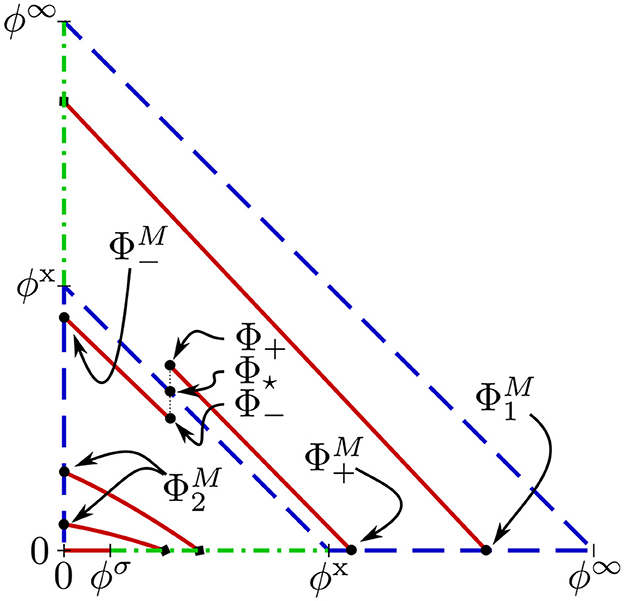
Figure 4. Different shock types for states connected to the origin. Continuous curves are 2-Lax shocks, dashed curves are 1-Lax shocks and dash-dotted are over-compressive shocks. The Hugoniot locus of the origin comprises the two edges and the contact manifolds $\mathcal{C}({\text{Φ}}^{\text{x}})$, $\mathcal{C}({\text{Φ}}^{\infty })$. Additionally, some 2-Lax shock curves from arbitrarily chosen generic points ${\text{Φ}}_1^M$, ${\text{Φ}}_2^M$, ${\text{Φ}}_{-}^M$, and ${\text{Φ}}_{+}^M$ are indicated. Reference values on the horizontal axis ∂¹ are ϕ^σ, ϕ^x, and ϕ^∞, on the vertical axis ∂² are ϕ^x and ϕ^∞. Recently, we became aware that the 2-Lax branch of $\mathcal{H}({\text{Φ}}_2^M)$ crossing the OC branch of $\mathcal{H}(O)$ corresponds to the fishbone structure that was studied in [36].

On the edge ∂², at Φ^x = (0,^ϕx)T and Φ^∞ = (0,^ϕ∞)T the shocks are 1-Lax and characteristic at the right states, say $\sigma (O,{\text{Φ}}^{\text{x}})={\text{λ}}_2({\text{Φ}}^{\text{x}})$ and $\sigma (O,{\text{Φ}}^{\infty })={\text{λ}}_2({\text{Φ}}^{\infty })$. On the edge ∂¹, at Φ^σ = (^{ϕσ, 0)T}, and Φ^x = (^{ϕx, 0)T} and Φ^∞ = (^{ϕ∞, 0)T} the shocks are 2-Lax (red and continuous) and 1-Lax, respectively, being characteristic at left or right states, say $\sigma (O,{\text{Φ}}^{\sigma })={\text{λ}}_1(O)$, $\sigma (O,{\text{Φ}}^{\text{x}})={\text{λ}}_2({\text{Φ}}^{\text{x}})$ and $\sigma (O,{\text{Φ}}^{\infty })={\text{λ}}_2({\text{Φ}}^{\infty })$. The over-compressive shocks (green and dot-dashed) are restricted in between Φ^σ and Φ^x on ∂¹ and in between Φ^x and Φ^∞ on ∂². Several states located in Figure 3B have characteristic shocks: If $\text{Φ}\in \mathcal{C}({\text{Φ}}^{\text{x}})$, then the shock is right characteristic for the second family. If ϕ = ϕ^∞, then it is characteristic for both families. If Φ = (0,^ϕσ)T, then the shock is 2-Lax but left characteristic in the first family.

6. Riemann problems

In this section, we construct the solution of the Riemann problems RP(O, Φ) and RP(Φ, Φ^∞), where O = (0, 0)^T, Φ^∞ ∈ ∂^∞, and $\text{Φ}\in {\mathcal{D}}_{{\text{Φ}}^{\infty }}$ is a generic right or left state in the phase space. These Riemann problems are derived from the standard initial condition (15).

6.1. The Riemann problem RP (O, Φ)

The behavior of solutions to the Riemann problem RP(O, Φ) depends on the position of Φ in the interior of ${\mathcal{D}}_{{\text{Φ}}^{\infty }}$ with respect to the contact manifold $\mathcal{C}({\text{Φ}}^{\text{x}})$, which divides the domain into two regions, see Figure 4:

$\begin{array}{l}{D}_{\text{x}}^{-}:=\{\text{Φ}\in D_{{\text{Φ}}^{\infty }}:\varphi <{\varphi }^{\text{x}}\},\\ D_{\text{x}}^{+}:=\{\text{Φ}\in D_{{\text{Φ}}^{\infty }}:\varphi >{\varphi }^{\text{x}}\},\end{array}$

where $\mathcal{C}({\text{Φ}}^{\text{x}})=\text{cl}({\mathcal{D}}_{\text{x}}^{-})\cap \text{cl}({\mathcal{D}}_{\text{x}}^{+})$ marks the intersection of the closures of those two regions. The main difference between both domains is the opposite direction of the characteristic speeds on the integral curves. In ${\mathcal{D}}_{\text{x}}^{-}$ the second eigenvalue increases from edge ∂¹ to edge ∂², and, reversely, in ${\mathcal{D}}_{\text{x}}^{+}$ it increases from edge ∂² to edge ∂¹. See the orientation of the second rarefactions in Figure 2A, where the arrows point into the directions of increasing eigenvalues.

A Riemann solution from O to any state Φ in ${\mathcal{D}}_{{\text{Φ}}^{\infty }}$ generally consists of a 1-Lax shock followed by a 2-Lax shock. For Φ belonging to ${\mathcal{D}}_{\text{x}}^{-}$ the middle state that connects the 1-wave with the 2-wave is denoted by ${\text{Φ}}_{-}^M$, and for Φ belonging to ${\mathcal{D}}_{\text{x}}^{+}$ the middle state is denoted by ${\text{Φ}}_{+}^M$. In both cases the middle state Φ^M belongs to the 1-Lax locus of the origin O. Since both waves are shocks any middle state ${\text{Φ}}_{+}^M$ or ${\text{Φ}}_{-}^M$ is located at $\mathcal{H}(\text{Φ})\cap \mathcal{H}(O)$. It turns out that ${\text{Φ}}_{+}^M$ belongs to the edge ∂¹ and ${\text{Φ}}_{-}^M$ belongs to the edge ∂².

For a right state $\text{Φ}\in {\mathcal{D}}_{\text{x}}^{-}$ the solution of RP(O, Φ) comprises the 1-Lax shock from O to a state Φ^M = (0,^ϕM)T such that ϕ^M ∈ (0, ϕ^x) and the 2-Lax shock from Φ^M to Φ. Similarly, for a right state $\text{Φ}\in {\mathcal{D}}_{\text{x}}^{+}$ the solution of RP(O, Φ) comprises the 1-Lax shock from O to a state Φ^M = (^{ϕM, 0)T} such that ϕ^M ∈ (ϕ^x, ϕ^∞) and the 2-Lax shock from Φ^M to Φ. Such cases are depicted in Figure 4; the former as ${\text{Φ}}_{-}\in {\mathcal{D}}_{\text{x}}^{-}$ and the latter as ${\text{Φ}}_{+}\in {\mathcal{D}}_{\text{x}}^{+}$.

We noticed a change in the nature of solution behavior when Φ crosses the contact manifold $\mathcal{C}({\text{Φ}}^{\text{x}})$. Such a bifurcation clearly occurs in the phase space, see also Figure 2B. However, in the solution profile the changes are smooth through this manifold. To do this, we need to understand the solution of the RP(O, Φ) with Φ in $\mathcal{C}({\text{Φ}}^{\text{x}})$. In [38], there is a detailed explanation of the ${\mathcal{L}}^1-$continuity of solutions as Φ changes along ${\mathcal{D}}_{{\text{Φ}}^{\infty }}$.

The solution of the Riemann problem RP(O, Φ) with Φ on the Hugoniot locus of O comprises a single shock from O to Φ with a classification that depends on the position of Φ and is elaborated in Theorem 2:

1. For Φ = (ϕ, 0)^T with ϕ ∈ (ϕ^σ, ϕ^x) the shock is over-compressive,

2. For Φ = (0, ϕ)^T with ϕ ∈ (ϕ^x, ϕ^∞) the shock is over-compressive,

3. For Φ = (ϕ, 0)^T with ϕ ∈ (0, ϕ^σ) the shock is 2-Lax,

4. For any other Φ in $\mathcal{H}(O)$ the shock is 1-Lax.

For a state $\text{Φ}\in \mathcal{C}({\text{Φ}}^{\text{x}})$, the solution of the Riemann problem RP(O, Φ) consists of a single 1-Lax shock from O to Φ. The two consecutive shocks from O to (0,^ϕx)T and from (0,^ϕx)T to Φ have both the same speed $v_1({\varphi }^{\text{x}})=v_2({\varphi }^{\text{x}})$, which in turn is the same speed of the direct shock from O to Φ. Since all these shocks have the same speed, the middle state (0,^ϕx)T is “invisible” in the solution profile in the physical space; this is because of Lemma 1. Therefore, the solution structure for $\text{Φ}\in {\mathcal{D}}_{{\text{Φ}}^{\infty }}$ is represented as

$O{\displaystyle \underset{}{\overset{1-\text{Lax}}{\to }}}{\text{Φ}}^M{\displaystyle \underset{}{\overset{2-\text{Lax}}{\to }}}\text{Φ}.$

For $\text{Φ}\in \mathcal{C}({\text{Φ}}^{\text{x}})$ the middle state Φ^M may assume any other state on the same contact manifold and even collapse with Φ. This is the basis of the ${\mathcal{L}}^1-$continuity in the solution profiles.

Please refer to Figure 4 and notice that as any ${\text{Φ}}_{-}\in {\mathcal{D}}_{\text{x}}^{-}$ tends to a $\text{Φ}\in \mathcal{C}({\text{Φ}}^{\text{x}})$ the middle state ${\text{Φ}}_{-}^M$ tends to (0,^ϕx)T. Similarly, as ${\text{Φ}}_{+}\in {\mathcal{D}}_{\text{x}}^{+}$ tends to a $\text{Φ}\in \mathcal{C}({\text{Φ}}^{\text{x}})$, the state ${\text{Φ}}_{+}^M$ tends to (^{ϕx, 0)T}. Thus, we notice a continuous dependence of solutions to the Riemann problem RP(O, Φ) on the right datum, even when it has a vivid bifurcation in the phase space.

6.2. The Riemann problem RP (Φ, Φ^∞)

In this Section, the dependence of the solution structure on the exponents n₁ and n₂ is illustrated by two examples: Example 1 and Example 2, with the corresponding parameter settings (44) and (60), respectively.

In Example 1, the solution consists of a simple 1-wave comprising a shock followed by a rarefaction or a single rarefaction. The solution structure of Example 2 depends on the existence of one or two detached inflection curves for the first characteristic family, which seem to emerge within the quasi-umbilic points Q₂ and Q₃ described in Appendix 1 (Supplementary material). As $\mathcal{C}({\text{Φ}}^{\infty })$ is a contact manifold, the goal is to consider a generic state $\text{Φ}\in {\mathcal{D}}_{{\text{Φ}}^{\infty }}$ from which waves reaching any state in Φ^∞∈∂^∞ are constructed. Remarkably, the solution structure for RP(O, Φ) remains the same for both examples.

Construction for Example 1. The construction for Example 1 can be orientated by the integral curves and the inflection manifold in Figure 2. In Figure 2A, the inflection manifold ${\mathcal{I}}_1$ of the first family is shown as a dash-dotted curve, which is almost a straight line, connecting the states ${{\text{Φ}}^{◇}}_1={(0.4,0)}^{\text{T}}$ and ${{\text{Φ}}^{◇}}_2={(0,0.5)}^{\text{T}}$. This can be compared to Lemma 6. Therefore, a wave curve starting at a state on the upper-right hand side of ${\mathcal{I}}_1$ follows a centered rarefaction of the first family until the maximum packing manifold ∂^∞ is reached. The final rarefaction point is (0, 1)^T, unless the starting state is on the ∂¹ axis, in such a case, the final rarefaction point is (1, 0)^T. Again, according to the triple shock rule over a contact manifold $\mathcal{C}({\text{Φ}}^{\infty })$, the latter may also be seen as finishing at (1, 0)^T. The clear bifurcation in the phase space does not exist in the solution profile.

The characteristic velocities near the contact manifold $\mathcal{C}({\text{Φ}}^{\infty })$ are close to zero, and the characteristic directions are close to $r_2=r_1={(1,-1)}^{\text{T}}$, see (43). If the left state Φ is on the lower-left side of the inflection ${\mathcal{I}}_1$ then the wave is obtained by a backward 1-wave construction. Namely, all shocks from a state Φ at the lower-left hand side of ${\mathcal{I}}_1$ are connected to a state ${\text{Φ}}^M\in \mathcal{H}(\text{Φ})$ on the right of ${\mathcal{I}}_1$ satisfying $\sigma (\text{Φ},{\text{Φ}}^M)={\text{λ}}_1({\text{Φ}}^M)$. Therefore, the solution for such a state Φ comprises the 1-Lax shock from Φ to Φ^M which is characteristic at Φ^M, and the rarefaction curve from Φ^M to (0, 1)^T, or (1, 0)^T if Φ belongs to ∂¹.

Construction of Example 2. In this example the parameters are specified as

$\begin{array}{ll}{v}_{1\infty }=1,v_{2\infty }=1/2,n_1=4.6,n_2=1.5.& (60)\end{array}$

The construction of Example 2 is visualized in Figure 5. For the study of the solution profiles, the growth direction of the slow eigenvalues along the integral curves is key in their structure for both examples RP(Φ, Φ^∞). Figure 5A shows the ${\mathcal{I}}_1$ inflection manifold in two detached parts called $\mathcal{T}$ and $\mathcal{B}$; we use the latter for the bottom part and the former for the top part. In $\mathcal{T}$, the inflection consists only of minimum eigenvalues. Point B possesses certain qualities, it is the limit of the integral curves that do not cross $\mathcal{B}$, from the edge ∂¹ to B, the eigenvalues are minimum, and from B to the maximum concentration, they are maximum.

FIGURE 5

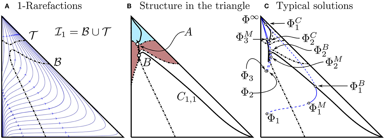
Figure 5. Curves of Example 2. In (A), the first family rarefaction curves are plotted as continuous curves, the arrows point into the direction of increasing eigenvalues. The dash-dotted curves are the inflection manifold ${\mathcal{I}}_1$ splitted into the two branches: $\mathcal{T}$ and $\mathcal{B}$. In (B), the solid curve C_1,1 is the double-contact of the first family (notice the two components, one in the light region and other in the white region); A is the state where a limit shock curve from $\mathcal{T}$ does not cross $\mathcal{B}$; it is tangent to it at B. In (C), the presentation of the wave curve solutions includes continuous curves corresponding to rarefaction fans and dashed curves corresponding to shock waves.

In Figure 5B the light (blue) and dark (brown) shaded regions represent right states Φ for which the solutions are similar to that of Example 1:

1. When the states belong to the upper corner above $\mathcal{T}$ within the light shaded region, then the wave curve comprises a single 1-rarefaction connecting the state Φ moving along increasing eigenvalues λ₁ toward Φ^∞ = (1, 0)^T;

2. For a left state Φ in the dark shaded region, a characteristic 1-Lax shock to a middle state in the light shaded region crosses $\mathcal{T}$, from this middle state a first family rarefaction follows to the maximum package concentration.

The construction of RP(Φ, Φ^∞) solutions for Φ in the white region of Figure 5B is outlined below. All solutions start with a right characteristic 1-Lax shock to a state ${\text{Φ}}^M\in \mathcal{H}(\text{Φ})$ such that $\sigma (\text{Φ},{\text{Φ}}^M)={\text{λ}}_1({\text{Φ}}^M)$. We distinguish three cases according to the number of flights over $\mathcal{B}$ or $\mathcal{T}$:

(1) The shock curve crosses $\mathcal{B}$ once;

(2) The shock curve crosses $\mathcal{T}$ once;

(3) The shock curve crosses $\mathcal{B}$ twice, and $\mathcal{T}$ once.

In Figure 5C, the left states of case (1) are represented by Φ₁ and Φ₂, case (2) are represented by left states Φ in the dark region of panel (b) (see point 2 above) and, case (3) are represented by Φ₃. The wave curves starting from Φ₁, Φ₂ and Φ₃ have the following structure:

$\begin{array}{ll}{\text{Φ}}_1\stackrel{\text{1-Lax}}{\to }\left|{\text{Φ}}_1^M\stackrel{\text{1-rar}}{\to }{\text{Φ}}_1^B\right|\stackrel{\text{1-Lax}}{\to }|{\text{Φ}}_1^C\stackrel{\text{1-rar}}{\to }{\text{Φ}}^{\infty },& (61)\end{array}$

$\begin{array}{ll}{\text{Φ}}_2\stackrel{\text{1-Lax}}{\to }\left|{\text{Φ}}_2^M\stackrel{\text{1-rar}}{\to }{\text{Φ}}_2^B\right|\stackrel{\text{1-Lax}}{\to }|{\text{Φ}}_2^C\stackrel{\text{1-rar}}{\to }{\text{Φ}}^{\infty },& (62)\end{array}$

$\begin{array}{ll}{\text{Φ}}_3\stackrel{\text{1-Lax}}{\to }|{\text{Φ}}_3^M\stackrel{\text{1-rar}}{\to }{\text{Φ}}^{\infty },& (63)\end{array}$

where the symbol | indicates where a shock is characteristic. For case (3) the construction of the shock curves proceeds as before, namely a 1-Lax shock followed by a 1-rarefaction connecting a middle state ${\text{Φ}}_3^M$ in the light shade region in Figure 5B to Φ^∞. For cases (1) and (2), the characteristic shock $({\text{Φ}}_i,{\text{Φ}}_i^M)$ precedes a 1-rarefaction from ${\text{Φ}}_i^M$ toward $\mathcal{B}$ at a state ${\text{Φ}}_i^B$ on C_{1, 1}, from there another 1-Lax left and right characteristic shock connects to a state ${\text{Φ}}_i^C$ on the other side of C_{1, 1}. From ${\text{Φ}}_i^C$ the wave curve terminates with a 1-rarefaction to Φ^∞.

If the state Φ₂ is approximated to a state Φ₃ then a continuous change in the solution profile is observed such that the wave group (62) collapses to the wave group (63). Indeed, if Φ₂ comes closer to Φ₃, then ${\text{Φ}}_2^M$ comes closer to ${\text{Φ}}_2^B$ and ${\text{Φ}}_2^C$ to ${\text{Φ}}_3^M$ in such a way that the shock speeds $\sigma ({\text{Φ}}_2,{\text{Φ}}_2^M)$ and $\sigma ({\text{Φ}}_2^B,{\text{Φ}}_2^C)$ approximate $\sigma ({\text{Φ}}_3,{\text{Φ}}_3^M)$, until, in the limit, the 1-rarefaction wave from ${\text{Φ}}_2^M$ to ${\text{Φ}}_2^B$ vanishes.

In Figure 6, the wave group for sedimentation with initial concentration ${\text{Φ}}_0={(0.1,0.2)}^{\text{T}}$ is shown as an example of solutions of the first type, which turns out to be most complete by an additional sequence of shocks upon crossing the double contact C_{1, 1}. The concentration profiles are depicted along the vertical direction, denoted by the dimensionless variable ξ = x/t, where the species experience gravitational effects to reach the base at x = L. In Figure 6A, a single shock for the setting of Example 1 can be observed, similarly as it occurs for Φ₃ of Example 2. Figure 6C shows the concentrations for the setting of Example 2. In this case, we can appreciate two 1-Lax shocks. The first shock, with the initial datum on the left and ${\text{Φ}}_1^M$ on the right, has velocity σ_1M. The second shock, denoted with a larger velocity σ_BC, crosses the double contact C_{1, 1} from ${\text{Φ}}_1^B$ to ${\text{Φ}}_1^C$.

FIGURE 6

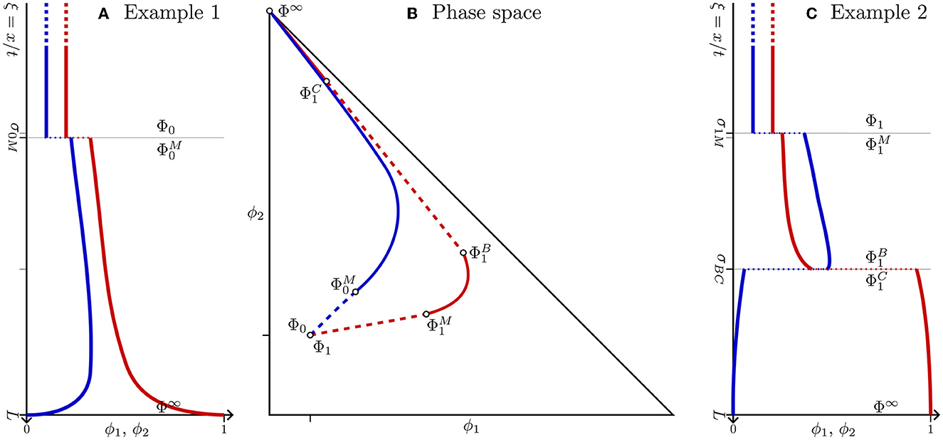
Figure 6. (A) Typical solution profile for Example 1, with parameters v_∞1 = 1, v_∞2 = 1/2, n₁ = 4, n₂ = 3; solid curves represent rarefaction fans, dashed curves correspond to shock waves; blue curves correspond to phase 1, red to phase 2; (B) path of the wave group in phase space plots: the blue curve represents the wave curve associated with Example 1, the red curve represents the path for the solution in Example 2; (C) typical solution profile for Example 2, with parameters v_1∞ = 1, v_2∞ = 1/2, n₁ = 4.6, n₂ = 1.5.

Why does the sediment rise from the very bottom with dominance of particles of phase 2 marked by red lines? A physically motivated explanation is that, although phase 2 by design has a smaller terminal velocity (v_∞2 < v_∞1), the smaller hindrance exponent (n₂ < n₁) compensates this by an overall larger settling velocity at large concentrations. If particle shape and density can be assumed to be the same, then the smaller terminal velocity, i.e., the Stokes velocity at vanishing concentrations, comes from a smaller particles size. However, at large concentrations approaching the maximum packing ∂^∞, the hindrance factor (8) becomes dominant in determining the settling velocity. Consequently, the smaller particles get attached to the bottom, whereas the bigger particles marked in blue color tend to settle upon them. Toward the sediment, lighter particles float above denser particles. The state Φ^∞ = (0, 1)^T at the very bottom means that the hindrance factor is the dominant and definitive criterion of the horizontal order of the phases.

Notably, the behavior of the sedimentation process is similar from ${\text{Φ}}_0^M$ to Φ^∞ in Example 1 and from ${\text{Φ}}_1^M$ to ${\text{Φ}}_1^B$ in Example 2. The rarefaction from ${\text{Φ}}_1^C$ to Φ^∞ has no counterpart in Example 1. However, this only occurs in the solution profiles, as noted in the central panel where both curves reach Φ^∞ with similar slopes. The change in convexity in the behavior of the sediment near the base is due to the different exponents in the hindered-settling velocities, as observed in the settings for each example given in Eqs. (44) and (60), respectively.

7. Discussion

We have successfully analyzed Riemann problem solutions related to particle sedimentation testing. The semi-analytical analysis for the solution of the RP(Φ, Φ^∞) shows that extending it to systems with more components is complicated, and its development requires a handcrafted approach as all the manifolds through which the solutions can bifurcate must be studied. Example 2 is an instance of this situation, say with the introduction of a double contact manifold C_{1, 1}. In several phase space dimensions more complicated situations can occur.

On the other hand, the study of the solution for RP(O, Φ) is much simpler and can be done analytically. This situation can be scaled to systems with several different particles as long as the conditions (S1) and (S2) are consistently scaled, namely v_∞1 > v_∞2 > ⋯ > v_∞N > 0 and n₁ > n₂ > ⋯ > n_N > 1, respectively. In these situations, the contact manifold has codimension one and is identified by a specific ϕ^x as in the Defs. 4 and 5 with the respective extension of Lemma 2. In particular, the family associated with the manifold depends on the type of codimension of the particular state in it. The inner points of this surface belong to a N-th contact manifold, its boundary of codimension 2 is a (N−1)-th contact manifold, this reduction of family continues until reaching the edges that represent a 2-th contact manifold. Still, $\mathcal{C}({\text{Φ}}^{\text{x}})$ is part of the Hugoniot locus of origin.

The solution is constructed by concatenating Lax shocks, whose position depends solely on the relative location of Φ in relation to $\mathcal{C}({\text{Φ}}^{\text{x}})$. When ϕ < ϕ^x, the 1-Lax shock usually occurs on the corresponding axis ∂^N, and for ϕ > ϕ^x, it typically occurs on the axis ∂¹. It is important to note that this may vary if Φ lies on the axes or, more generally, if ϕ_k = 0 for some k ∈ 1, …, N. Preliminary examples show that for N = 3, the construction can be achieved using a simple algorithm. Starting from Φ, we can calculate its Hugoniot locus and obtain the Φ^M′ state: If ϕ < ϕ^x is satisfied, then ${\varphi }_3^{M^{\prime }}$ is set to 0, and if ϕ > ϕ^x, then ${\varphi }_1^{M^{\prime }}$ is set to 0; this yields a 3-Lax shock. From Φ^M′, we can find Φ^M at the corresponding boundary, as discussed above. Thus, the sought-after solution is given by the sequence

$O{\displaystyle \underset{}{\overset{1-\text{Lax}}{\to }}}{\text{Φ}}^M{\displaystyle \underset{}{\overset{2-\text{Lax}}{\to }}}{\text{Φ}}^{M^{\prime }}{\displaystyle \underset{}{\overset{3-\text{Lax}}{\to }}}\text{Φ}.$

There is currently limited knowledge regarding the analysis of umbilic points for systems with more than two equations. The investigation of quasi-umbilic and DRS points (see [39, 40]) presents great potential for advancing our understanding in this research field. The initial identification of DRS points on the elliptic/hyperbolic boundary is provided in Čanić [41]. A comprehensive discussion on the additional connections between these points can be found in the Supplementary material.

Data availability statement

The original contributions presented in the study are included in the article/Supplementary material, further inquiries can be directed to the corresponding author.

Author contributions

All authors listed have made a substantial, direct, and intellectual contribution to the work and approved it for publication.

Funding

This work was supported by Conacyt (National Council for Science and Technology of Mexico) through the Basic Science program with Grant A1-S-26012. We would also like to thank Conicyt (Chile) for their support through Fondecyt project #1120587. SB acknowledges the support of Universidad del Bío-Bío through project INES I+D 22-14 (Co-construyendo un ecosistema para la transformación digital y el desarrollo territorial de las Regiones de Biobío y Ñuble) and ANID (Chile) for support through Fondecyt project #1230560.

Acknowledgments

We would like to extend our sincere appreciation to the editor for their professionalism and valuable input in shaping this work. We are also grateful to the reviewers whose feedback greatly improved the presentation and content of the manuscript. Additionally, we thank ITAM for their installations and partial support from Asociación de Cultura Mexicana A.C.

Conflict of interest

The authors declare that the research was conducted in the absence of any commercial or financial relationships that could be construed as a potential conflict of interest.

Publisher's note

All claims expressed in this article are solely those of the authors and do not necessarily represent those of their affiliated organizations, or those of the publisher, the editors and the reviewers. Any product that may be evaluated in this article, or claim that may be made by its manufacturer, is not guaranteed or endorsed by the publisher.

Supplementary material

The Supplementary Material for this article can be found online at: https://www.frontiersin.org/articles/10.3389/fams.2023.1199011/full#supplementary-material

References

1. Berres S, Bürger R, Karlsen KH, Tory EM. Strongly degenerate parabolic-hyperbolic systems modeling polydisperse sedimentation with compression. SIAM J Appl Math. (2003) 64:41–80. doi: 10.1137/S0036139902408163

CrossRef Full Text | Google Scholar

2. Bürger R, Karlsen KH, Tory EM, Wendland WL. Model equations and instability regions for the sedimentation of polydisperse suspensions of spheres. Z Angew Math Mech. (2002) 82:699–722. doi: 10.1002/1521-4001(200210)82:10<699::AID-ZAMM699>3.0.CO;2-#

CrossRef Full Text | Google Scholar

3. Benzoni-Gavage S, Colombo RM. An n-populations model for traffic flow. Eur J Appl Math. (2003) 14:587–612. doi: 10.1017/S0956792503005266

CrossRef Full Text | Google Scholar

4. Berres S, Ruiz-Baier R, Schwandt H, Tory E. An adaptive finite-volume method for a model of two-phase pedestrian flow. Netw Het Media. (2011) 6:401–23. doi: 10.3934/nhm.2011.6.401

CrossRef Full Text | Google Scholar

5. Berres S, Bürger R. On Riemann problems and front tracking for a model of sedimentation of polydisperse suspensions. Z Angew Math Mech. (2007) 87:665–91. doi: 10.1002/zamm.200710343

CrossRef Full Text | Google Scholar

6. Berres S, Bürger R. On the settling of a bidisperse suspension with particles having different sizes and densities. Acta Mecanica. (2008) 201:47–62. doi: 10.1007/s00707-008-0072-0

CrossRef Full Text | Google Scholar

7. Biesheuvel PM. Particle segregation during pressure filtration for cast formation. Chem Eng Sci. (2000) 55:2595–606. doi: 10.1016/S0009-2509(99)00536-9

CrossRef Full Text | Google Scholar

8. Masliyah JH. Hindered settling in a multiple-species particle system. Chem Eng Sci. (1979) 34:1166–8.

Google Scholar

9. Basson DK, Berres S, Bürger R. On models of polydisperse sedimentation with particle-size-specific hindered-settling factors. Appl Math Modell. (2009) 33:1815–35. doi: 10.1016/j.apm.2008.03.021

CrossRef Full Text | Google Scholar

10. Richardson JF, Zaki WN. Sedimentation and fluidization: part I. Trans Inst Chem Engrs. (1954) 32:35–53.

Google Scholar

11. Dafermos CM. Hyperbolic Conservation Laws in Continuum Physics. Berlin: Springer Verlag (2000).

Google Scholar

12. Donat R, Mulet P. A secular equation for the Jacobian matrix of certain multi-species kinematic flow models. Num Methods Partial Diff Equat. (2010) 26:159–75. doi: 10.1002/num.20423

CrossRef Full Text | Google Scholar

13. Berres S, Voitovich T. On the spectrum of a rank two modification of a diagonal matrix for linearized fluxes modelling polydisperse sedimentation. In:Tadmor E, , editor. Hyperbolic Problems. Theory, Numerics and Applications. College Park, MD: American Mathematical Society (AMS) (2009). p. 409–18.

Google Scholar

14. Bürger R, Donat R, Mulet P, Vega CA. Hyperbolicity analysis of polydisperse sedimentation models via a secular equation for the flux Jacobian. SIAM J Appl Math. (2010) 70:2186–213. doi: 10.1137/09076163X

CrossRef Full Text | Google Scholar

15. Castañeda P, Furtado F, Marchesin D. On singular points for convex permeability models. In:Ancona F, Bressan A, Marcati P, Marson A, , editors. Hyperbolic Problems: Theory, Numerics, Applications. Springfield, MO: American Mathematical Society (AMS) (2014). p. 415–422.

Google Scholar

16. Isaacson E, Marchesin D, Plohr B, Temple B. The Riemann problem near a hyperbolic singularity: the classification of solutions of quadratic Riemann problems. SIAM J Appl Math. (1988) 48:1009–32.

Google Scholar

17. Isaacson E, Marchesin D, Plohr B, Temple B. Multiphase flow models with singular Riemann problems. Mat Apl Comput. (1992) 11:147–66.

Google Scholar

18. Matos V, Castañeda P, Marchesin D. Classification of the umbilic point in immiscible three-phase flow in porous media. In:Ancona F, Bressan A, Marcati P, Marson A, , editors. Hyperbolic Problems: Theory, Numerics, Applications. Springfield, MO: American Mathematical Society (AMS) (2014). p. 791–9.

Google Scholar

19. Schaeffer DG, Shearer M. The classification of 2 x 2 systems of non-strictly hyperbolic conservation laws with application to oil recovery. Comm Pure and Appl Math. (1987) 40:141–78.

Google Scholar

20. Fayers FJ. Extension of Stone's method 1 and conditions for real characteristic three-phase flow. SPE Reservoir Eng. (1989) 4:437–45.

Google Scholar

21. Isaacson E, Temple B. Analysis of a singular hyperbolic system of conservation laws. J Differ Equ. (1986) 65:250–68.

Google Scholar

22. Abreu E, Matos V, Perez J, Rodriguez-Bermadez P. A class of Lagrangian-Eulerian shock-capturing schemes for first-order hyperbolic problems with forcing terms. J Sci Comput. (2021) 86:14. doi: 10.1007/s10915-020-01392-w

CrossRef Full Text | Google Scholar

23. Castañeda P, Abreu E, Furtado F, Marchesin D. On a universal structure for immiscible three-phase flow in virgin reservoirs. Comput Geosci. (2016) 20:171–85. doi: 10.1007/s10596-016-9556-5

CrossRef Full Text | Google Scholar

24. Azevedo AV, de Souza AJ, Furtado F, Marchesin D, Plohr B. The solution by the wave curve method of three-phase flow in virgin reservoirs. Transp Porous Media. (2010) 83:99–125. doi: 10.1007/s11242-009-9508-9

CrossRef Full Text | Google Scholar

25. Tang J, Castañeda P, Rossen WR, Marchesin D. Three-phase fractional-flow theory of foam-oil displacement in porous media with multiple steady states. Water Resour Res. (2019) 55:10319–39. doi: 10.1029/2019WR025264

CrossRef Full Text | Google Scholar

26. Rodríguez-Bermúdez P, Marchesin D. Riemann solutions for vertical flow of three phases in porous media: simple cases. J Hyperbolic Differ Equ. (2013) 10:335–70. doi: 10.1142/S0219891613500124

CrossRef Full Text | Google Scholar

27. de Souza AJ. Stability of singular fundamental solutions under perturbations for flow in porous media. Mat Aplic Comp. (1992) 11:73–115.

Google Scholar

28. Schecter S, Marchesin D, Plohr B. Structurally stable Riemann solutions. J Differ Equ. (1996) 126:303–54.

Google Scholar

29. Schecter S, Plohr BJ, Marchesin D. Classification of codimension-one Riemann solution. J Dyn Diff Equ. (2001) 13:523–88. doi: 10.1023/A:1016634307145

CrossRef Full Text | Google Scholar

30. Azevedo AV, Marchesin D, Plohr B, Zumbrun K. Capillary instability in models for three-phase flow. Zeitschrift für Angewandte Mathematik und Physik. (2002) 53:713–46. doi: 10.1007/s00033-002-8180-5

CrossRef Full Text | Google Scholar

31. Lozano Guerrero LF, Marchesin D. Diffusive Riemann solutions for 3-phase flow in porous media. In: CNMAC 2019 - XXXIX Congresso Nacional de Matematica Aplicada e Computacional. Uberlândia (2020). p. 7.

Google Scholar

32. Majda A, Pego RL. Stable viscosity matrices for systems of conservation laws. J Diff Equ. (1985) 56:229–62.

Google Scholar

33. Rodríguez-Bermúdez P, Marchesin D. Loss of strict hyperbolicity for vertical three-phase flow in porous media. In:Ancona F, Bressan A, Marcati P, Marson A, , editors. Hyperbolic Problems: Theory, Numerics, Applications. Springfield, MO: American Mathematical Society (AMS) (2014). p. 881–8.

Google Scholar

34. Furtado F. Structural stability of nonlinear waves for conservation laws. PhD thesis. New York University, New York, NY, United States (1989).

Google Scholar

35. Lax P. Hyperbolic systems of conservation laws II. Commun Pure Appl Math. (1957) 10:537–66.

Google Scholar

36. Matos V, Azevedo AV, Mota JCD, Marchesin D. Bifurcation under parameter change of Riemann solutions for nonstrictly hyperbolic systems. Z Angew Math Phys. (2015) 66:1413–52. doi: 10.1007/s00033-014-0469-7

CrossRef Full Text | Google Scholar

37. Temple B. Systems of conservation laws with invariant submanifolds. Trans Am Math Soc. (1983) 280:781–95.

Google Scholar

38. Berres S, Castañeda P. Identification of shock profile solutions for bidisperse suspensions. Bull Braz Math Soc. (2016) 47:105–15. doi: 10.1007/s00574-016-0125-2

CrossRef Full Text | Google Scholar

39. Dumortier F, Roussarie R, Sotomayor J. Generic 3-Parameter Families of Vector Fields: Unfoldings of Saddle, Focus, and Elliptic Singularities with Nilpotent Linear Parts. Berlin; Heidelberg; New York, NY: Springer-Verlag (1991).

Google Scholar

40. Azevedo AV, Marchesin D, Plohr B, Zumbrun K. Bifurcation of nonclassical viscous shock profiles from the constant state. Commun Math Phys. (1999) 202:267–90.

Google Scholar

41. Čanić S. On the influence of viscosity on Riemann solutions. J Dyn Differ Equ. (1998) 10:109–49.

Google Scholar