MAD (about median) vs. quantile-based alternatives for classical standard deviation, skewness, and kurtosis

1. Introduction

Classical statistics uses the standard deviation σ as the primary measure of dispersion. In computing σ, we use the squares of the distances from the mean μ. As noted in [1], using the L₂ norm is convenient in differentiation, estimation, and optimization. The additive property of variance σ² for independent variables is also cited as one of the prime reasons for using the L₂ norm in sampling theory and analysis of variance. A historical survey is given in [2].

At the same time, this norm has a number of disadvantages. For example, large deviations from outliers contribute heavily to mean and standard deviation and could significantly overestimate “typical” deviations. A natural alternative is to use the L₁ norm and measure absolute deviations from a central point such as the mean or median.

The idea of using the L₁ norm is not new. The L₁ norm was considered independently by both Boscovitch and Laplace as early as the eighteenth century. A historical survey using the L₁ norm is presented in [3, 4] and a survey of more recent results is given in [1]. However, the L₁ norm has not been widely used in statistics and statistical modeling [1].

There is currently a renewed interest in using the L₁ norm for robust statistical modeling and inference [e.g., [5–9]]. Using the L₂ norm, the influence of outliers is even more magnified when computing skewness and kurtosis as these computations would involve raising means and standard deviation to 3^rd and 4^th powers. By contrast, using mean absolute deviations from the mean or median (both denoted as MAD in literature) can be more appropriate. Therefore, using the L₁ norm, outliers will have less influence on the results. Consequently, results from using the MAD (mean absolute deviation) are more robust to outliers than those obtained using the standard deviation, as is common in classical statistics.

Throughout this paper, we will use MAD to denote the mean absolute deviation from the median. We will use the MAD in deriving alternative expressions for skewness and kurtosis. The proposed MAD-based measures can be computed and interpreted as sub-means of the appropriate left and right sub-ranges. The obtained formulas are analogous to those used in statistics based on quantiles.

The MAD-based alternative measures considered in this paper use only the first-order moment. Consequently, they do not overweight outliers as compared to classical measures. When compared to the quantile metrics, they are more sensitive to concentrations at the extreme ends of distributions. In addition, these alternative measures have many desirable characteristics, such as scale (by absolute value) and/or shift-invariance.

We illustrate our results with several examples. One of the novel contributions of this paper is the MAD-based alternative metric for kurtosis. This metric is shown to be in the [0, 1] range, allowing us to compare the data distribution with different numerical scales. We present a detailed analysis of some well-known distributions. We contrast the proposed MAD-based metrics with both quantile and classical statistics metrics.

2. Organization of the paper

This paper is organized as follows. Section 3 introduces notation and reviews some bounds on mean absolute deviation. In Section 4, we focus on computing MAD, show how it can be computed as a difference of corresponding sub-means, and contrast the expression for MAD deviation with that of quartile deviation. In Section 5, we introduce MAD-based skewness and kurtosis. The MAD expression for skewness has been known before. To our knowledge, the proposed expression for MAD-based kurtosis has not been considered before. Both MAD-based skewness and kurtosis have simple interpretations, and their formulas are similar to quantile-based alternatives skewness and kurtosis. Section 6 discusses the advantages of proposed measures vs. corresponding classical and quantile-based measures. Section 7 focuses on computational considerations and shows how MAD-based measures can be computed from some integrals related to the underlying probability distributions. In Section 8, we provide a detailed comparison for a number of distributions:

1. Continuous uniform (Section 8.1)

2. Normal (Section 8.2)

3. Log-normal (Section 8.3)

4. Exponential (Section 8.4)

5. Laplace (Section 8.5)

6. Pareto (section 8.6).

In Section 9, we present an example of applying our results to analyze wealth distribution. In Section 10, we directly compare MAD-based skewness and kurtosis for the above six distributions. We conclude our paper with Section 11.

For completeness and clarity of presentation, we moved some details of derivations into Appendices. In Appendix 1 (Section A1), we present summary tables for the above distributions. In Appendices 2–4 (Sections A2–A4) we present some computational details for log-normal, Laplace and Pareto distributions, respectively.

3. Preliminaries

We start with preliminary definitions. Consider a real-valued random variable X on a sample space Ω⊆R with density f(x), finite mean E(X), and cumulative distribution function F(x). If X is a discrete random variable, then Ω is some countable sample space, and f(x) is the probability mass function (discrete density function).

We use μ = E(X) and σ to denote mean and standard deviation of X. Let F⁻¹ be the quantile function defined by F⁻¹(t) = inf{x:F(x) ≥ t} with t ∈ [0, 1]. The median M, the quartiles Q₁ and Q₃ are given by M = F⁻¹(1/2), $Q_1=F^{-1}(1/4)$, and $Q_3=F^{-1}(3/4)$, respectively.

For any a, we define the mean absolute deviation of X from a as

$\begin{array}{ll}H(X,a)=E(|X-a|)={\displaystyle {\int }_{\Omega }}|x-a|f(x)dx& (1)\end{array}$

If a = μ, then H(X, μ) is the mean absolute deviation from the mean μ. If we take a = M, then H(X, M) is the mean absolute deviation from the median. Both of these are denoted as MAD (mean absolute deviation) in the statistical literature, leading to some confusion [1]. In this paper, we use MAD to denote mean absolute deviations from the median. It can be interpreted as the average distance of values of X to the median M. We will write H as an abbreviation to H(X, M).

Let us start by establishing a lower and upper bound for H. Since f(x) ≥ 0, is integrable and E(X) < ∞ we have −|x − M|f(x) ≤ (x − M)f(x) ≤ |x − M|f(x) and, therefore, we obtain

$\begin{array}{l}H={\displaystyle {\int }_{\Omega }}|x-M|f(x)dx\ge |{\displaystyle {\int }_{\Omega }}(x-M)f(x)dx|=|M-\mu |\end{array}$

To establish an upper bound, we use the well-known fact that H ≤ H(X, a) for any value of a [10–12]. In particular, if a = μ then H ≤ E(|X − μ|). This means that the average absolute deviation from the median H is always less than or equal to the mean absolute deviation from the mean E(|X − μ|). If we apply Jensen's inequality E(g(X)) ≥ g(μ) to the convex function g(t) = t² (corresponding to σ²) we immediately obtain an upper bound for H:

$\begin{array}{l}{\sigma }^2=\text{E}({(X-\mu )}^2)=\text{E}(g(|X-\mu |))\ge g\left[\text{E}(|X-\mu |)\right]\\ ={\left[\text{E}(|X-\mu |)\right]}^2\ge H^2\end{array}$

Of the three metrics to measure deviations, namely H, E(|X − μ|) and σ, the MAD metric H has the lowest value.

Example 1: Consider two uniform random variables X and Y with corresponding sample spaces Ω_x and Ω_y with n = 12 elements given by

$\begin{array}{l}{\Omega }_X=\{1,2,3,4,5,6,7,8,9,10,11,12\},\text{ and}\\ {\Omega }_Y=\{1,2,3,4,5,6,7,8,9,10,11,100\}\end{array}$

and the discrete density functions f_x(·) = f_y(·) = 1/n for any value in Ω_X and Ω_Y, respectively. For variable X we have M_x = 6.5, μ_x = 6.5, σ_x = 3.45, and H_x = 3 whereas for variable Y we have M_y = 6.5, μ_y = 13.83, σ_y = 26.16, and H_y = 10.33. For the purpose of illustration, let us define an outlier as any numeric value v with |v − μ| > 2σ. Both random variables X and Y have the same median M_x = M_y = 6.5, but the random variable Y has a much higher outlier value y₁₂ = 100. This much higher outlier value results in a higher mean and a higher standard deviation for Y than for X. The impact of this outlier value on H can be immediately computed: it increases H from H_x = 3 to H_y = 10.33 by (y₁₂ − x₁₂)/n = 7.33. The change in standard deviations due to this outlier would involve a much more complicated expression. The MAD-based deviation H_Y for Y is about four times higher than the MAD-based deviation H_x for X, whereas the standard deviation σ_y for Y, is more than seven times greater than σ_x for X because of the squaring of the deviations. To assess the impact of the outlier y₁₂ = 100, we compare H_x and H_y in terms of σ_x and σ_y. For variable X we have H_x ≈ 0.87σ_x whereas for variable Y we have H_y ≈ 0.39σ_y. The lower value of H_y as compared with σ_y for Y indicates that Y has heavier tails compared to X.

The above example with an outlier illustrates one of the advantages of using MAD instead of standard deviation as a measure of variability. When computing the standard deviation or variance of X, the outlier effect is amplified since we square the differences (x_i − μ). This effect of outliers is further amplified in computing skewness or kurtosis where we need to raise these differences to the 3^rd or 4^th power. By contrast, the proposed MAD-based metrics for deviation, skewness, and kurtosis is easy to interpret and express in terms of simple differences and ratios of mean absolute deviations computed over corresponding sub-ranges of X. As a result, these measures are less impacted by outliers than the corresponding measures used in classical statistics.

Another advantage of using mean absolute deviation H instead of standard deviation σ is that H is often simpler to interpret as it is computed directly (without squaring). Consider the example suggested in [1]: if X follows a uniform distribution in [0, 1] then H = 1/4 and $\sigma =\sqrt{3}/2$ (for details see Section 8.1). The MAD value H = 1/4 is easy to interpret: it represents the average distance of X from its median M = 1/2. However, it is more difficult to find an easy interpretation for standard deviation $\sigma =\sqrt{3}/2$.

4. MAD computation and interpretation

Our approach is to replace standard deviation σ with mean absolute deviation from the median H and to derive MAD-based measures for skewness and kurtosis without resorting to higher powers. The proposed measures are simple to interpret in terms of corresponding sub-ranges.

We will find it convenient to use the indicator function for any subset U ⊂ Ω

$\begin{array}{l}{1}_U=\{\begin{array}{cc}1\hfill & \text{if }x\in U\hfill \\ 0& \text{otherwise}\end{array}\hfill \end{array}$

Define the left sub-space of Ω by Ω^L = {w ∈ Ω|x(w) ≤ M} and right sub-space of Ω by Ω^R = {w ∈ Ω|x(w) > M}. Also, define $X^L=X{1}_{{\Omega }^L}$ and $X^R=X{1}_{{\Omega }^R}$. Then, from the definition of H in Equation (1) we have

$\begin{array}{l}H={\displaystyle {\int }_{\Omega }}|x-M|f(x)dx={\displaystyle {\int }_{{\Omega }^L}}(M-x)f(x)dx\end{array}$

$\begin{array}{ll}+{\displaystyle {\int }_{{\Omega }^R}}(x-M)f(x)dx=\text{E}(X^R)-\text{E}(X^L)& (2)\end{array}$

From the above equation, it is easy to show that for any constants b and c we have H(bX + c) = |b|H and, therefore, H is shift invariant. In addition, from Equation (2), we can interpret H as the difference of the sub-means of the right sub-range Ω^R and left sub-range Ω^L. Since E(X) = E(X^L)+E(X^R), we have H = E(X)−2E(X^L). Therefore, we can also interpret H as the difference between the mean of X and twice the sub-mean of X^L.

Let us now compare the mean absolute deviation H in Equation (2) with quartile deviation (or semi-quartile range) H_Q = (Q₃ − Q₁)/2 which is used in descriptive statistics as a measure of statistical dispersion [e.g., [13, 14]]: Both equations for H and H_Q have the same form under this correspondence:

$\begin{array}{ll}\text{E}(X^L)\iff Q_1/2\text{and E}(X^R)\iff Q_3/2& (3)\end{array}$

Example 2: Consider the same random variable X uniform in Ω = {1, 2, …, 12} as in the previous example. For this sequence n = 12, f(x) = 1/12, E(X) = M = 6.5, and H = 3. Let us re-compute H using the left and right half sub-ranges. To that end, we split Ω into left and right sub-spaces (Ω^L and Ω^R) around the median:

$\begin{array}{l}\Omega =\{{\displaystyle \underset{{\Omega }^L(\text{left half})}{{\displaystyle \underbrace{1,2,3,4,5,6}}}},{\displaystyle \underset{{\Omega }^R(\text{right half})}{{\displaystyle \underbrace{7,8,9,10,11,12}}}}\}\end{array}$

For the left sub-mean, we have $\text{E}(X{1}_{{\Omega }^L})=(1+2+3+4+5+6)/12=1.75$ and for the right sub-mean $\text{E}(X{1}_{{\Omega }^R})=(7+8+9+10+11+12)/12=4.75$. Then we compute H = E(X^R)−E(X^L) = 3. Alternatively, we have H = E(X)−2E(X^L) = 3. To compute the corresponding quantile-based metric H_Q, we note that the first and third quartiles for this sequence are Q₁ = 3.75 and Q₃ = 9.25. Therefore, the quantile-based deviation H_Q = (Q₃ − Q₁)/2 = 2.75.

5. MAD-based alternatives for skewness and kurtosis

We now consider skewness and kurtosis. In classical statistics, skewness is defined as a measure of the asymmetry of the probability distribution around its mean. For a survey, see [15]. One of the most common measures is the moment coefficient of skewness (or skew) S, defined as the third standardized moment in terms of mean μ and standard deviation σ, namely,

$\begin{array}{ll}S=\frac{E{(X-\mu )}^3}{{\sigma }^3}& (4)\end{array}$

Just like in the computation of variance, this definition is sensitive to outliers. We will define MAD-based alternatives for skewness and kurtosis without resorting to the computation of higher powers. In this way, our proposed expressions for skewness and for kurtosis will be more resilient to outliers.

We proceed as follows. From Equation (2), the expression for H can be written as follows:

$\begin{array}{ll}H=\text{E}((M-X)1_{{\Omega }^L})+\text{ E}((X-M)1_{{\Omega }^R})& (5)\end{array}$

The first term is the contribution to H from $X{1}_{{\Omega }^L}$ whereas the second term is the contribution to H from X1_{Ω^R. Our MAD-based alternative A_M for skewness can be defined as the (normalized) difference of these contributions as follows:

$\begin{array}{ll}{A}_M=\frac{\text{E}((X-M)1_{{\Omega }^R})-\text{E}((M-X)1_{{\Omega }^L})}{H}& (6)\end{array}$

The above expression immediately implies that the MAD-based skewness is both shift and translation invariant.

From Equation (2), we can re-write the expression for A_M in Equation (6) as follows:

$\begin{array}{ll}{A}_M=\frac{\text{E}(X)-M}{H}& (7)\end{array}$

Therefore, the MAD-based metric A_M for skewness coincides with Groeneveld and Meeden's skewness coefficient [16]. The MAD-based skewness in Equation (7) has a simple interpretation as the ratio of two distances: the numerator E(X)−M is the (signed) distance between the mean and the median, whereas the numerator H is the average distance of values in X to the median. It is more difficult to attach a simple and intuitive interpretation to the classical skewness S in Equation (4).

Let us compare the MAD-based skewness from the above Equation (7) with the non-parametric skewness given by (E(X)−M)/σ. Since H ≤ σ, we have the following relationship between these measures:

$\begin{array}{l}\text{Non Parametric Skewness }=\frac{\text{E}(X)-M}{\sigma }\le A_M\end{array}$

Next, we derive the upper and lower bound for A_M. Since $\text{E}((X-M)1_{{\Omega }^L})<0$ and $\text{E}((X-M)1_{{\Omega }^R})>0$ from Equations (5) and (6) we easily obtain −1 ≤ A_M ≤ 1.

The definition of MAD-based skewness in Equation (6) has been suggested before [e.g., [17]]. However, our results for the representation of H would allow us to derive simple computational expressions for MAD-skewness and compare the obtained results with skewness estimates used in quantile statistics.

To start, let us re-write our definition of A_M as follows. From Equation (6), we obtain

$\begin{array}{ll}{A}_M=\frac{(\text{E}(X^R)-M/2)-(M/2-\text{E}(X^L))}{\text{E}(X^R)-\text{E}(X^L)}& (8)\end{array}$

We can now compare MAD-based skewness A_M from Equation (8) with the quantile skewness A_Q often used in descriptive statistics [e.g., [18, 19]]:

$\begin{array}{ll}{A}_Q=\frac{(Q_3-M)-(M-Q_1)}{Q_3-Q_1}=\frac{(Q_3/2-M/2)-(M/2-Q_1/2)}{Q_3/2-Q_1/2}& (9)\end{array}$

where Q_i denote the corresponding quartiles. The expressions in Equations (8) and (9) have the same form under the same correspondence as before in Equation (3). The numerator in Equation (9) for A_Q is the difference between the average of upper and lower quartiles and the median and the denominator is the quartile deviation H_Q. By contrast, in Equation (8) for A_M, the numerator is the difference between the concentrations of probability mass for the left and right halves and the half median, whereas the denominator is the mean absolute deviation H.

Finally, note that from Equation (9) we have

$\begin{array}{l}{A}_Q=-1+\frac{2(Q_3-M)}{Q_3-Q_1}\ge -1and{A}_Q=1-\frac{2(M-Q_1)}{Q_3-Q_1}\le 1\end{array}$

Therefore, both MAD-based skewness A_M and quantile-based skewness A_Q are always in the range [−1, 1]. By contrast, the classical skewness S can be unbounded.

We now turn our attention to kurtosis. Recall that classical Pearson's kurtosis K is defined as [20]:

$\begin{array}{ll}K=\frac{E{(X-\mu )}^4}{{\sigma }^4}& (10)\end{array}$

To define an analogy to kurtosis using absolute deviations from the median, we find it useful to interpret kurtosis as suggested in [21]. We consider a standardized variable Z = (X − μ)/σ and let W = Z². Then E(W) = 1 and

$\begin{array}{l}\text{Var}(W)=\text{E}(W^2)-{\text{E}}^2(W)=K-1\Rightarrow K=\text{Var}(W)+1\end{array}$

Note that since Z is normalized and dimensionless, W = Z² is also automatically dimensionless. Therefore, Var(W) is also dimensionless. The kurtosis K can be viewed then as related to the dispersion of W = Z² around its mean 1. Equivalently, K is associated with the dispersion of Z around −1 and 1 [21]. This implies that kurtosis is associated with the concentration of X around points μ−σ and μ+σ. High values of kurtosis can occur in a peaked unimodal distribution, in a dual-peaked bi-modal distribution, or with the concentration of probability in the tails of the distribution.

Pursuing this analogy, we want to define MAD-based kurtosis to measure the concentration of X around Q₁ (playing the role of μ−σ) and around Q₃ (playing the role of μ+σ) as in classical statistics.

Consider Ω^L and Ω^R defined above. We measure the concentration of probability in Ω^L around Q₁ by $\text{E}(|X-Q_1|1_{{\Omega }^L})$.

Similarly, we measure the concentration of probability in Ω^R around Q₃ by $\text{E}(|X-Q_3|1_{{\Omega }^R})$. We define MAD-based alternative T_M for kurtosis by normalizing the total concentration by MAD:

$\begin{array}{ll}{T}_M=\frac{\text{E}(|X-Q_1|1_{{\Omega }^L})+\text{E}(|X-Q_3|1_{{\Omega }^R})}{H}& (11)\end{array}$

From the above definition, it is easy to show that MAD-based kurtosis T_M is scale and translation invariant just as MAD-based skewness A_M.

The above expression for T_M in Equation (11) can be interpreted as follows. From the definition of the median, F(X^L) = F(X^R) = 0.5. Therefore, the term E(|X − Q₁|1_{{X ≤ M}}) in Equation (11) can be interpreted as one half of the average distance d_L of values of X^L from Q₁. Similarly, the term E(|X − Q₃|1_{{X > M}}) in Equation (11) can be interpreted as one half of the average distance d_R of values of X^R from Q₃. The numerator in Equation (11) is then the average of these distances, namely (d_L + d_R)/2.

Therefore, the proposed MAD-based alternative T_M for kurtosis in Equation (11) has a simple and intuitive explanation as the ratio of two distances: the numerator is the average of distances from values in Ω^L and Ω^R from Q₁ and Q₃, respectively, whereas the denominator H is the average distance of values of Ω to its median M. It is more difficult to provide an intuitive explanation of the classical kurtosis K in Equation (10).

Let us now establish some simple bounds for T_M. Recall that the median minimizes the sum of absolute deviations [11, 12]. Since Q₁ is the median for X^L and Q₃ is the median for X^R, we obtain $\text{E}(|X-Q_1|1_{{\Omega }^L})\le \text{E}((M-X)1_{{\Omega }^L})$ and $\text{E}(|X-Q_3|1_{{\Omega }^R})\le \text{E}((X-M)1_{{\Omega }^R})$. Therefore, from (11) we can immediately obtain:

$\begin{array}{l}0\le T_M\le \frac{\text{E}((M-X)1_{{\Omega }^L})+\text{E}((X-M)1_{{\Omega }^R})}{H}=1\end{array}$

Unlike Pearson's kurtosis K that can be unbounded [22], the proposed MAD-based alternative T_M for kurtosis is always in the range 0 ≤ T_M ≤ 1. This could allow for more meaningful comparisons of data.

The definition of MAD-based measures to measure tails has been suggested before [17]. In that work, it was suggested to use $\text{E}((M-X)1_{{\Omega }^L})/H$ and $\text{E}((X-M)1_{{\Omega }^R})/H$ as measures of fat tails. By contrast, our suggestion for MAD-based kurtosis in Equation (11) is to use the mean absolute deviations of left and right sub-spaces from their corresponding medians Q₁ and Q₃, not from the median M. This would allow us to provide additional interpretation for the proposed kurtosis and to compare the proposed formula for T_M with quantile kurtosis T_Q suggested by Moors [21].

To proceed, let us re-write T_M in terms of sub-means of corresponding sub-means. We consider the following sub-spaces:

$\begin{array}{l}\begin{array}{c}{\Omega }^{LL}=\left\{w\in \Omega |x(w)\le Q_1\right\},{\Omega }^{LR}=\left\{w\in \Omega |Q_1\le x(w)\le M\right\},\hfill \\ {\Omega }^{RL}=\left\{w\in \Omega |M\le x(w)\le Q_3\right\},{\Omega }^{RR}=\left\{w\in \Omega |x(w)\ge Q_3\right\}\hfill \end{array}\hfill \end{array}$

and define

$\begin{array}{l}{X}^{LL}=X{1}_{{\Omega }^{LL}},X^{LR}=X{1}_{{\Omega }^{LR}},\\ X^{RL}=X{1}_{{\Omega }^{RL}},X^{RR}=X{1}_{{\Omega }^{RR}}\end{array}$

From the above definitions, we have

$\begin{array}{l}\text{E}(|X-Q_1|1_{\left\{X\le M\right\}})=\text{E}(X^{LR})-\text{E}(X^{LL}),\\ \text{E}(|X-Q_3|1_{\left\{X>M\right\}})=\text{E}(X^{RR})-\text{E}(X^{RL})\end{array}$

and therefore, we can re-write our expression (11) for kurtosis T_M as follows

$\begin{array}{ll}{T}_M=\frac{\text{E}(X^{LR})-\text{E}(X^{LL})+\text{E}(X^{RR})-\text{E}(X^{RL})}{E(X^R)-E(X^L)}& (12)\end{array}$

Moors [21] suggested a quantile-based formula for kurtosis in terms of the octiles O₁, …, O₇ as follows:

$\begin{array}{ll}{T}_Q=\frac{(O_7-O_5)+(O_3-O_1)}{(O_6-O_2)}& (13)\end{array}$

The expressions in Equations (12) and (13) have the same form under the following correspondence:

$\begin{array}{l}\begin{array}{c}\text{E}(X^{LR})-\text{E}(X^{LL})\iff \frac{(O_3-O_1)}{2},\\ \text{E}(X^{RR})-\text{E}(X^{RL})\iff \frac{(O_7-O_5)}{2},\\ E(X^R)-E(X^L)\iff \frac{(O_6-O_2)}{2}\end{array}\end{array}$

Our justification for (12) is analogous to the justification for a quantile-based alternative to kurtosis in (13) in terms of octiles suggested in [21]. The terms in the numerator of T_Q are large if large probability mass is concentrated in O₂ and O₆ corresponding to large dispersion around μ−σ and μ+σ. The terms in the numerator of T_M. are small if small probability mass is concentrated in Q₁ and Q₃. The difference between our formula in (12) and the quantile-based formula in (13) is that we measure these masses in terms of “partial” means E(X^LL), E(X^LR), E(X^RL) and E(X^RR) instead of octiles. This is illustrated in the following example.

Example 3: As before, consider a random variable X with uniform probability in Ω = {1, 2, …, 12}. The corresponding sub-ranges are shown below:

$\begin{array}{l}\Omega ={\displaystyle \underset{{\Omega }^L(\text{left half})}{{\displaystyle \underbrace{\stackrel{{\Omega }^{LL}(1^{st}\text{ quarter})}{\overbrace{1,2,3}},\stackrel{{\Omega }^{LR}(2^{nd}\text{ quarter})}{\overbrace{4,5,6}}}}}},{\displaystyle \underset{{\Omega }^R(\text{right half})}{{\displaystyle \underbrace{\stackrel{{\Omega }^{RL}(3^{rd}\text{ quarter})}{\overbrace{7,8,9}},\stackrel{{\Omega }^{RR}(4^{th}\text{ quarter})}{\overbrace{10,11,12}}}}}}\end{array}$

For this sequence, we compute H = 3. This distribution is symmetric and S = A_M = A_Q = 0. We will therefore focus on MAD-based kurtosis T_M. The median for the left sub-range Ω^L is Q₁ = 3.5 and we compute $H(X^L,Q_1)=0.75$. The value $H(X^L,Q_1)=1.5$ is one half of the average distance d_L from values in Ω^L to its median Q₁. Similarly, the median for the right sub-range Ω^R is Q₃ = 9.5 and we compute $H(X^R,Q_3)=0.75$. The value $H(X^R,Q_3)=1.5$ is one half of the average distance d_R from values in Ω^R to its median Q_R. Therefore, the term $H(X^L,Q_1)+H(X^R,Q_3)=(d_L+d_R)/2=0.75$ is the average of the distances from sub-ranges Ω^L and Ω^R to their respective median. From Equation (11) the MAD-based kurtosis T_M = 0.5. It has a simple interpretation as the ratio of the average distances (d_L + d_R)/2 to H which is the average distance of Ω to its median M = 6.5. Let us re-compute T_M using sub-means. We have E(X^LL) = 0.5, E(X^LR) = 1.25, E(X^RL) = 2 and E(X^RR) = 2.75. Applying Equation (12) we have T_M = 0.5. By contrast, the standard statistical kurtosis is K = 1.78. Let us compare the MAD-based kurtosis T_M with quantile-based kurtosis T_Q in formula (13). To compute T_Q, we compute the octiles O₁, …, O₇ for our sequence (using midpoint for interpolation): O₁ = 2.375 O₂ = 3.75, O₃ = 5.125, O₄ = 6.5, O₅ = 7.875, O₆ = 9.25 and O₇ = 10.625. Then, the quantile formula for kurtosis from Equation (13) gives us T_Q = 1.

6. Discussion

One of the reasons to use quantile-based metrics for data is that they are resistant to outliers. One of the measures of this resistance is the sample breakdown point - the proportion of observations that can be altered that can result in statistics being arbitrarily large or small. The median M has a breakpoint of 50%. This means that 50% of the points must be “outliers” before the median can be moved outside the range of outliers [9, 23]. By contrast, the breakpoint of the mean is 0%. This means that a single observation would change it.

The computation of MAD-based measures for deviation, skewness, and kurtosis involves computing the corresponding sub-spaces. A single change in observation value would change these measures. However, these changes will not be as dramatic as changes for the classical measures.

By contrast, the MAD-based measures are determined by the corresponding sub-means. Any change in values would change some of these, and this, in turn, would result in different values for MAD-based measures for each of the sub-spaces. Note that a single observation value change would change the corresponding partial mean without affecting other sub-means. By contrast, a single change in observation would change the mean and result in changes for the corresponding moments, affecting both skewness and kurtosis. However, because the proposed MAD-based measures involve only the first moment whereas classical skewness and kurtosis involve the 3^rd and 4^th moments, respectively, we would expect that MAD-based measures would change by a smaller percentage than the corresponding classical measures.

For illustration, consider the MAD-based alternative T_M for kurtosis. It can capture concentrations in the tails more accurately than can the quantile kurtosis T_Q. For example, if the largest 10% of values in X increase in value then this cannot be captured by T_Q since octiles will not change. Similarly, if the smallest 10% of values in X decrease, then again octiles will not change resulting in the same value for octile kurtosis. By contrast, the proposed MAD-based formula for kurtosis uses sub-means of appropriate sub-ranges and can, therefore, more accurately reflect the impact of such larger or smaller values.

Schematically, we can indicate this as follows:

$\begin{array}{l}\Omega ={\displaystyle \underset{{\Omega }^L(\text{left half})}{{\displaystyle \underbrace{\stackrel{{\Omega }^{LL}(1^{st}\text{ quarter})}{\overbrace{\dots O_1\dots }}{Q}_1\stackrel{{\Omega }^{LR}(2^{nd}\text{ quarter})}{\overbrace{\dots O_3\dots }}}}}},\\ M,{\displaystyle \underset{{\Omega }^R(\text{right half})}{{\displaystyle \underbrace{\stackrel{{\Omega }^{RL}(3^{rd}\text{ quarter})}{\overbrace{\dots O_5\dots }}{Q}_3\stackrel{{\Omega }^{RR}(4^{th}\text{ quarter})}{\overbrace{\dots O_7\dots }}}}}}\end{array}$

If we consider any changes in values in quarter sub-ranges Ω^LL, Ω^LR, Ω^RL or Ω^RR that do not change the octiles, then the quantile kurtosis T_Q would remain the same. By contrast, these changes in values will change the corresponding sub-means and, therefore the value of MAD-based kurtosis T_M. Therefore, MAD-based kurtosis T_M can capture changes in probability mass in the tails more accurately than using octiles in T_Q.

By the same argument, it is easy to show that quantile skewness A_Q and quantile deviations H_Q would remain unchanged, whereas the mean absolute deviation from median H and MAD-based skewness A_M would change.

The proposed MAD-based alternative measures for deviation, skewness, and kurtosis provide additional tools for data analysis. These measures are less sensitive to outliers in that they change by a smaller percentage as compared to the changes in the classical statistics metrics.

At the same time, they do not ignore outliers as quantile-based measures do. In situations where classical, MAD-based, and quantile-based kurtosis could be computed, MAD-based kurtosis T_M has the advantage of 0 ≤ T_M ≤ 1, whereas both the classical kurtosis S could be unbounded. For some distributions such as log-normal, the quantile-based kurtosis could be unbounded as well (see Section 8.3). Using the proposed MAD-based alternative measure for kurtosis with a value that is always in [0, 1] provides a potentially useful tool to directly compare distributions in terms of the concentration of data in the tails.

As one potentially important application of these proposed measures considers the national income and wealth distributions [24]. It is widely recognized that there are disproportionate concentrations of income and wealth at the highest quantile. As the above example illustrates, the MAD-based metrics appear to have the ability to characterize concentrations in the upper-most quantiles in a manner that is not possible with the classical and quantile-based methods. This ability likely follows from the property that the MAD-based metrics are sensitive to excessive concentrations in the upper-most quantile, while the quantile-based metrics are not. At the same time, the classical metrics that use the third and fourth moment may overly exaggerate the impact of these concentrations in the upper-most quantile. The foregoing analysis demonstrates that these alternative MAD-based metrics would be able to capture the detailed behavior that is engendered by the concentrations of extreme income and wealth at the highest range of distribution, namely the highest quantile. We illustrate this by a detailed example in Section 9.

7. Computational considerations

In the computation of quantile-based measures, we need to compute the quantiles. These can be obtained from the inverse of the cumulative distribution function F⁻¹(p). The quartiles Q₁, M and Q₃ are obtained as $Q_1=F^{-1}(1/4)$, M = F⁻¹(1/2) and $Q_3=F^{-1}(3/4)$ whereas the remaining octiles are $O_i=F^{-1}(i/8)$ for i = 1, 3, 5, 7. Then the quantile-based measures for deviation, skewness, and kurtosis are

$\begin{array}{l}{H}_Q=\frac{Q_3-Q_1}{2},A_Q=\frac{Q_3+Q_1-2M}{(Q_3-Q_1)},\end{array}$

$\begin{array}{ll}{T}_Q=\frac{(O_7-O_5)+(O_3-O_1)}{(O_6-O_2)}& (14)\end{array}$

If the distribution is symmetric, the skewness A_Q = 0 and for octiles we have O₁ = 2M − O₇, Q₁ = 2M − Q₃, and O₃ = 2M − O₅. In particular, (O₇ − O₅) = (O₃ − O₁). In this case, we only need to compute four quantiles, namely M, O₅, Q₃ and Q₇ to obtain

$\begin{array}{ll}{H}_Q=Q_3-Mand{T}_Q=\frac{2(O_7-O_5)}{(Q_3-M)}& (15)\end{array}$

Note that the quantile-based measures are expressed in terms of differences of corresponding quantiles. This implies, in particular, that the above quantile-based measures in Equation (14) are shift-invariant.

In the computation of MAD-based performance measures, we need to compute the corresponding sub-means. To facilitate this computation, consider the following auxiliary integral:

$\begin{array}{l}I(z)={\displaystyle {\int }_{t\le z}}tf(t)dt\end{array}$

If we can evaluate the above integral for I(Q₁), I(M), and I(Q₃) then we can compute MAD-based performance measures from these integrals and the mean value E(X). Specifically, E(X^L) = I(M) and E(X^R) = E(X)−I(M). For the other sub-means, we have $\text{E}(X^{LL})=I(Q_1)$, $\text{E}(X^{LR})=I(M)-I(Q_1)$, $\text{E}(X^{RL})=I(Q_3)-I(M)$, and $\text{E}(X^{RR})=\text{E}(X)-I(Q_3)$. From this, we obtain the following for MAD-based deviation, skewness and kurtosis:

$\begin{array}{l}H=\text{E}(X)-2I(M),A_M=\frac{\text{E}(X)-M}{\text{E}(X)-2I(M)},\end{array}$

$\begin{array}{ll}{T}_M=\frac{\text{E}(X)+2I(M)-2I(Q_1)-2I(Q_3)}{\text{E}(X)-2I(M)}& (16)\end{array}$

In some situations, it is easier to evaluate the following integral

$\begin{array}{l}J(z)={\displaystyle {\int }_{t\ge z}}tf(t)dt\end{array}$

Since J(z) = E(X)−I(z), we can compute MAD-based deviation, skewness, and kurtosis as follows:

$\begin{array}{l}H=2J(M)-\text{E}(X),A_M=\frac{\text{E}(X)-M}{2J(M)-\text{E}(X)},\end{array}$

$\begin{array}{ll}{T}_M=\frac{2J(Q_1)+2J(Q_3)-2J(M)-\text{E}(X)}{2J(M)-\text{E}(X)}& (17)\end{array}$

The computation of MAD-based performance measures requires the computation of I(Q₁), I(M) and I(Q₃) in addition to computing the expected value E(X). By contrast, in classical statistics, to compute skewness, we need to compute expectation E(X), standard deviation σ, and the third moment E(X³). To compute Pearson's kurtosis would require us also to compute the fourth moment E(X⁴). Therefore, the computational cost of computing these measures is not higher than that of computing Pearson measures of classical statistics. Moreover, unlike the classical measures, the computation of MAD-based measures requires only the existence of first-order moments. For example, consider Pareto distributions with parameter α (see Section 8.6). For such distributions, the mean is defined for α > 1, variance is defined for α > 2, and kurtosis is defined for α > 3. By contrast, MAD-based measures would require only α > 1. Therefore, for 1 < α < 2 we can only use MAD-based or quantile-based measures to analyze deviation, skewness, and kurtosis.

On the other hand, we should note that there are situations where classical kurtosis K or MAD kurtosis T_M does not exists but the quantile-based kurtosis T_Q exists and is finite. An example is presented in [21]. If X follows the Cauchy distribution, its expected value, variance, and kurtosis are undefined. However, the quantile-based kurtosis T_Q is finite with T_Q = 2.

In most situations where classical, MAD-based, and quantile-based kurtosis could be computed, MAD-based kurtosis T_M has the advantage of 0 ≤ T_M ≤ 1 whereas the classical kurtosis K can be unbounded. For some distributions such as log-normal, the quantile-based kurtosis T_Q could also be unbounded (see Section 8.3 below for details). Using a MAD-based measure T_M for kurtosis with a value in 0 ≤ T_M ≤ 1 allows an additional comparison of all distributions in terms of their tails.

8. Comparisons for distributions

We now turn our attention to some well-known distributions. We will compute MAD-based alternatives for deviation, skewness, and kurtosis and compare them with the corresponding quantile-based and classical metrics for the following well-known probability distributions: continuous uniform, normal, log-normal, exponential, Laplace, and Pareto distributions. A summary table is provided in Section 1.

8.1. Continuous uniform distribution

Suppose X is distributed according to a uniform distribution in [a, b]. Its density f(x) = 1/(b − a) and its cumulative distribution function F(x) = (x − a)/(b − a). For this distribution, E(X) = M = (a + b)/2, $\sigma =(b-a)/2\sqrt{3}$ and K = 9/5. Since this distribution is symmetric, the skewness measures are 0.

The quantiles are computed from F⁻¹(p) = (1 − p)a + pb. In particular, Q₁ = (3a + b)/4, M = (a + b)/2 and Q₃ = (a + 3b)/4. Since this distribution is symmetric, we compute the octiles O₁ = (7a + b)/8, O₃ = (5a + 3b)/6, O₅ = (3a + 5b)/8 and O₇ = (a + 7b)/8. To compute MAD-based measures, consider the following integral

$\begin{array}{l}J(z)={\displaystyle {\int }_a^z}tf(t)dt=\frac{z^2-a^2}{2(b-a)},a\le z\le b\end{array}$

We have $J(Q_1)=(Q_1^2-a^2/2(b-a)$, J(M) = (M² − a²)/2(b − a) and $J(Q_3)=(Q_3^2-a^2)/2(b-a)$. From this using Equation (17) and Equation (15) we compute MAD-based and quantile-based measures for deviation and kurtosis. The results are summarized in the Table 1.

TABLE 1

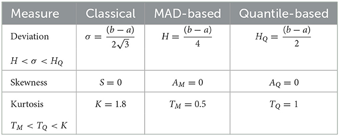
Table 1. A comparison of measures for uniform distribution.

8.2. Gaussian distribution

Suppose X is distributed according to normal distribution N(μ, σ²) with density f(x) and cumulative distribution function F(x):

$\begin{array}{l}f(x)=\frac{1}{\sigma \sqrt{2\pi }}{e}^{-{(x-\mu )}^2/2{\sigma }^2},\\ F(x)=\Phi \left(\frac{x-\mu }{\sigma }\right)=\frac{1}{\sigma \sqrt{2\pi }}{\displaystyle {\int }_{-\infty }^x}{e}^{-{(t-\mu )}^2/2{\sigma }^2}dt\end{array}$

where Φ(·) denotes the cumulative distribution of the standard normal. Let Q₁ and Q₃ denote the first and third quartiles of the standard normal distribution. This distribution is symmetric; therefore, all skewness measures are 0.

The MAD-based, quantile-based, and classical measures are invariant under shifts. Skewness and kurtosis are also invariant under scaling whereas for MAD-based deviation, H(X/σ) = (1/σ)H(X). Therefore, we can consider the standard normal distribution for X and multiply the obtained value for H(X) by 1/σ.

The quartiles for this distribution Q₃ = −Q₁ ≈ 0.67 whereas for the octiles we have O₅ = −O₃ ≈ 0.32, Q₃ = −Q₁ ≈ 0.68 and O₇ = −O₁ ≈ 0.15. To compute MAD-based MAD-based measures, consider the following integral

$\begin{array}{l}J(z)={\displaystyle {\int }_z^{\infty }}tf(t)dt=\frac{1}{\sqrt{2\pi }}{\displaystyle {\int }_z^{\infty }}t{e}^{-t^2/2}dt=\frac{1}{\sqrt{2\pi }}{e}^{-z^2/2}\end{array}$

Since Q₃ = −Q₁ ≈ 0.67 we have $J(Q_1)=J(Q_3)=exp(-Q_3^2/2)/\sqrt{2\pi }$ and $J(0)=1/\sqrt{2\pi }$. Therefore, from the above, using Equation (17) and Equation (15) we compute MAD-based and quantile-based measures for deviation and kurtosis. The results are summarized in Table 2.

TABLE 2

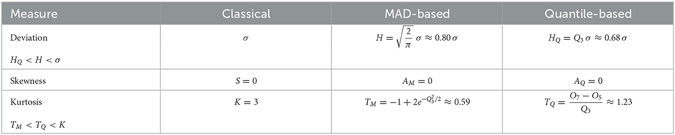
Table 2. A comparison of measures for normal distribution.

8.3. Log-normal distribution

Suppose X is distributed according to log-normal distribution with parameters μ ∈ (∞, +∞) and σ² (σ > 0). Its density f(x) and its cumulative distribution function F(x) are given by

$\begin{array}{l}f(x)=\frac{1}{x\sigma \sqrt{2\pi }}{e}^{-{(logx-\mu )}^2/2{\sigma }^2},\text{and}F(x)=\Phi \left(\frac{logx-\mu }{\sigma }\right)\end{array}$

where Φ(·) is the cumulative distribution function of the standard normal.

We will use the apostrophe ′ to distinguish the performance measures of X in the log-normal distribution from those of the underlying normal distribution. Therefore, σ′ will denote the standard deviation of X, μ′ will denote the mean of X etc. As before, let O_i denote the octiles of the standard normal and let $O_i^{\prime }$ denote the octiles of the log-normal distribution. Then $O_i^{\prime }=e^{\mu +\sigma O_i}$. In particular, the log-normal median is M′ = e^μ and the log-normal mean is μ′ = e^μ+σ2/2. Similarly, let Q₁ and Q₃ denote the first and third quartiles for the standard normal distribution and let $Q_1^{\prime }$ and $Q_3^{\prime }$ denote the corresponding quartiles for the log-normal distribution. Consider the following integral (derived in Appendix A2)

$\begin{array}{l}I(z)={\displaystyle {\int }_0^z}tf(t)dt={\mu }^{\prime }\Phi \left(\frac{logz-\mu }{\sigma }-\sigma \right)\end{array}$

In particular, $I(Q_1^{\prime })={\mu }^{\prime }(1-\Phi (\sigma -Q_1)$, I(M′) = μ′(1 − Φ(σ)) and $I(Q_3^{\prime })={\mu }^{\prime }(1-\Phi (\sigma -Q_3))$. Therefore, from the above, using Equation (17) and Equation (15) we compute MAD-based and quantile-based measures for deviation and kurtosis. Note that we can express mean absolute deviation H′ in terms of the error function erf(·). Using $\text{erf}(x)=2\Phi (x\sqrt{2})-1$ we obtain $H^{\prime }=2{\mu }^{\prime }\text{erf}(\sigma /\sqrt{2})$.

In Appendix A2, we show the following relationships between MAD-based and quantile-based measures:

$\begin{array}{l}{H}_Q^{\prime }<H^{\prime }\le {\sigma }^{\prime },A_M^{\prime },A_Q^{\prime }<S^{\prime },T_M^{\prime }<T_Q^{\prime }<K^{\prime }\end{array}$

We summarize our results in Table 3. In addition, in Appendix A2, we examined the asymptotic behavior of these measures for σ ↦ 0 and for σ ↦ ∞. For σ ↦ 0 we have $A_M^{\prime }\mapsto 0$, $T_M^{\prime }\mapsto 0.59$, $A_Q^{\prime }\mapsto 0$ and $T_Q^{\prime }\mapsto 1.23$. Therefore, for σ ↦ 0, the MAD-based and quantile-based measures for skewness and kurtosis converge to the corresponding values for normal distribution. On the other hand, for σ ↦ ∞

TABLE 3

Table 3. A comparison of measures for log-normal distribution.

we have: $A_M^{\prime }\mapsto 1$, $T_M^{\prime }\mapsto 1$, $A_Q^{\prime }\mapsto 1$ and $T_Q^{\prime }\mapsto \infty$. Finally, note that for log-normal distribution both quantile kurtosis $T_Q^{\prime }$ and classical kurtosis K′ are unbounded whereas the MAD-based kurtosis $T_M^{\prime }$ always satisfies $0\le T_M^{\prime }\le 1$. This allows us to compare distribution in the tails across different distributions. The results are summarized in Table 3.

8.4. Exponential distribution

Suppose X is distributed according to an exponential distribution with rate λ > 0 [22]. Its density f(x) = λe^−λx and its cumulative distribution function F(x) = 1 − e^−λx with x ∈ [0, ∞). Its mean E(X) = 1/λ and its standard deviation σ = 1/λ. The quantiles of exponential distribution are F⁻¹(p) and are given by −log(1 − p)/λ. In particular, Q₁ = log(4/3)/λ, M = log(2)/λ and Q₃ = log(4)/λ whereas the octiles are O₁ = log(8/7)/λ, O₃ = log(8/5)/λ, O₅ = log(8/3)/λ and O₇ = log(8)/λ.

To compute MAD-based measures, we compute (using integration by parts) the following integral

$\begin{array}{l}I(z)={\displaystyle {\int }_0^z}tf(t)dt={\displaystyle {\int }_0^z}\lambda t{e}^{-\lambda t}dt=\frac{1-(1+\lambda z)e^{-\lambda z}}{\lambda }\end{array}$

We compute I(Q₁) = (1 − 3log(4/3))/4λ, I(M) = (1 − log2)/2λ and I(Q₃) = (3 − log4)/4λ. Then from the above results and from Equations (16 a)nd (15) we compute MAD-based and quantile-based measures for deviation, skewness, and kurtosis. The results are summarized in the Table 4.

TABLE 4

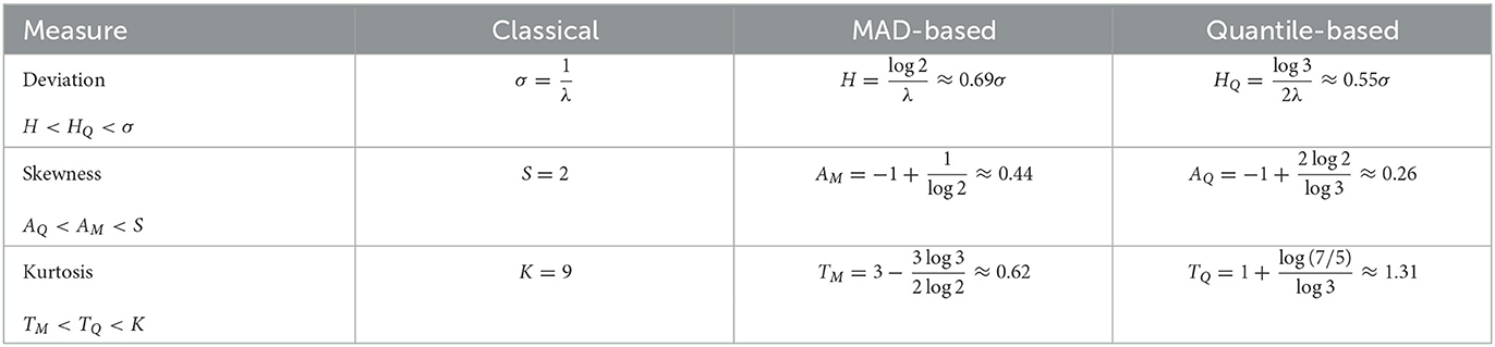
Table 4. A comparison of measures for exponential distribution.

8.5. Laplace distribution

Suppose X is distributed according to Laplace distribution with location μ and scale b. Its density f(x) and cumulative distribution function F(x) are given by Feller [22]

$\begin{array}{l}f(x)=\frac{1}{2b}{e}^{-|x-\mu |/b}\text{ and }F(x)=\{\begin{array}{c}\frac{1}{2}{e}^{(x-\mu )/b},ifx\le \mu \\ 1-\frac{1}{2}{e}^{-(x-\mu )/b},ifx\ge \mu \end{array}\end{array}$

This distribution of X is symmetric around μ. its median M and mean E(X) are both the same with E(X) = M = μ. Its standard deviation $\sigma =b\sqrt{2}$. Since both MAD-based measures and quantile-based measures are shift-invariant, we let μ = 0.

The quantiles are easily computed as F⁻¹(p). In particular, Q₁ = −blog2 and Q₃ = blog2. whereas for the octiles we have O₁ = −2blog2, O₃ = blog3 − 2blog2, O₅ = 2blog2−blog3, and O₇ = 2blog2.

To compute the MAD-based measures, we compute the integral J(z) (derived in Appendix A3):

$\begin{array}{l}J(z)={\displaystyle {\int }_z^{\infty }}xf(x)dx=\{\begin{array}{c}\frac{(b+z)}{2}{e}^{-z/b},z\ge 0\\ \frac{(b-z)}{2}{e}^{z/b},z<0\end{array}\end{array}$

We compute J(Q₁ = b(1 + log2)/4, J(M) = b/2 and J(Q₃) = b(1 + log2)/4. Then from Equations (17) and (15) we can compute MAD-based and quantile-based measures for deviation, skewness, and kurtosis. We summarize our results in Table 5.

TABLE 5

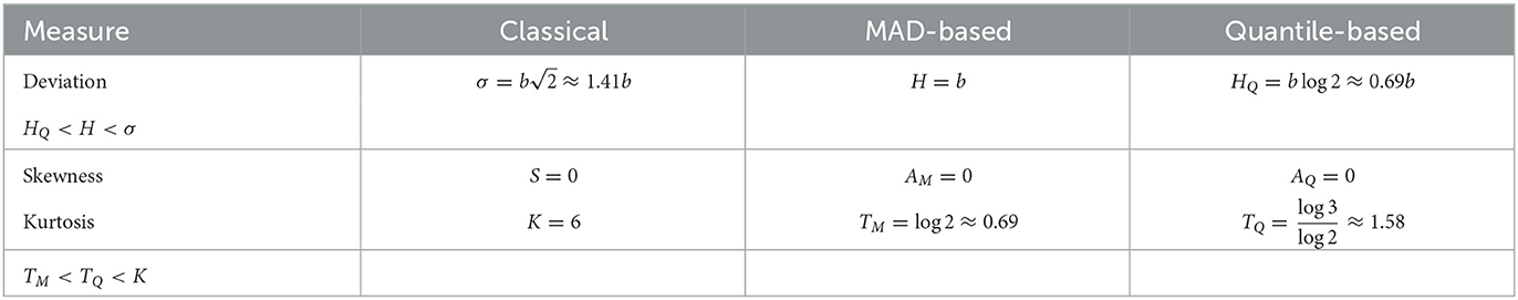
Table 5. A comparison of measures for Laplace distribution.

We note that just as for classical kurtosis, the MAD-based kurtosis for Laplace distribution is greater than the MAD-based kurtosis for Normal distribution. This is because the Laplace distribution has fatter tails compared to the Normal distribution.

8.6. Pareto distribution

Suppose X is distributed according to Pareto Type I distribution distribution with shape α > 0 and scale β > 0. Its density f(x) and its cumulative distribution function F(x) are given by

$\begin{array}{l}f(x)=\{\begin{array}{c}\frac{\alpha {\beta }^{\alpha }}{x^{\alpha +1}}x\ge \beta \\ 0x<\beta \end{array}\text{ and }F(x)=\{\begin{array}{c}1-{(\frac{\beta }{x})}^{\alpha }x\ge \beta \\ 0x<\beta \end{array}\end{array}$

This distribution has infinite mean μ for α ≤ 1, undefined variance σ² for α ≤ 2, undefined skewness S for α ≤ 3 and undefined (excess) kurtosis K for α ≤ 4. The quantiles are computed from F⁻¹(p) and are given by β/(1 − p)^1/α. For Q₁, M and Q₃ we have $Q_1=\beta \sqrt[\alpha ]{4/3}$, $M=\beta \sqrt[\alpha ]{2}$ and $Q_3=\beta \sqrt[\alpha ]{4}$. For the octiles we have $O_1=\sqrt[\alpha ]{8/7}$, $O_3=\sqrt[\alpha ]{8/5}$, $O_5=\sqrt[\alpha ]{8/3}$ and $O_7=\sqrt[\alpha ]{8}$. To compute MAD-based measures, we compute the integral for any z > = β and α > 1

$\begin{array}{l}J(z)={\displaystyle {\int }_z^{\infty }}xf(x)dx=-\frac{\alpha {\beta }^{\alpha }}{(1-\alpha )}{x}^{-\alpha +1}{|}_z^{\infty }=\frac{\alpha z}{(\alpha -1)}{(\frac{\beta }{z})}^{\alpha }\\ =\frac{\alpha z(1-F(z))}{(\alpha -1)}\end{array}$

Since 1 − F(Q₁) = 3/4, 1 − F(M) = 1/2, and 1 − F(Q₃) = 1/4, we immediately compute J(Q₁) = 3αβQ₁/4(α − 1), J(M) = αβM/2(α − 1), and J(Q₃) = αβQ₃/3(α − 1). Then from Equations (17) and (15) we can compute MAD-based and quantile-based measures for deviation H_Q, skewness A_Q, and kurtosis T_Q. Moreover, in Appendix (Section A4), we showed the following relationship between measures: H_Q < H < σ and A_Q < A_M < S and T_M < T_Q < K. These results are summarized in Table 6.

TABLE 6

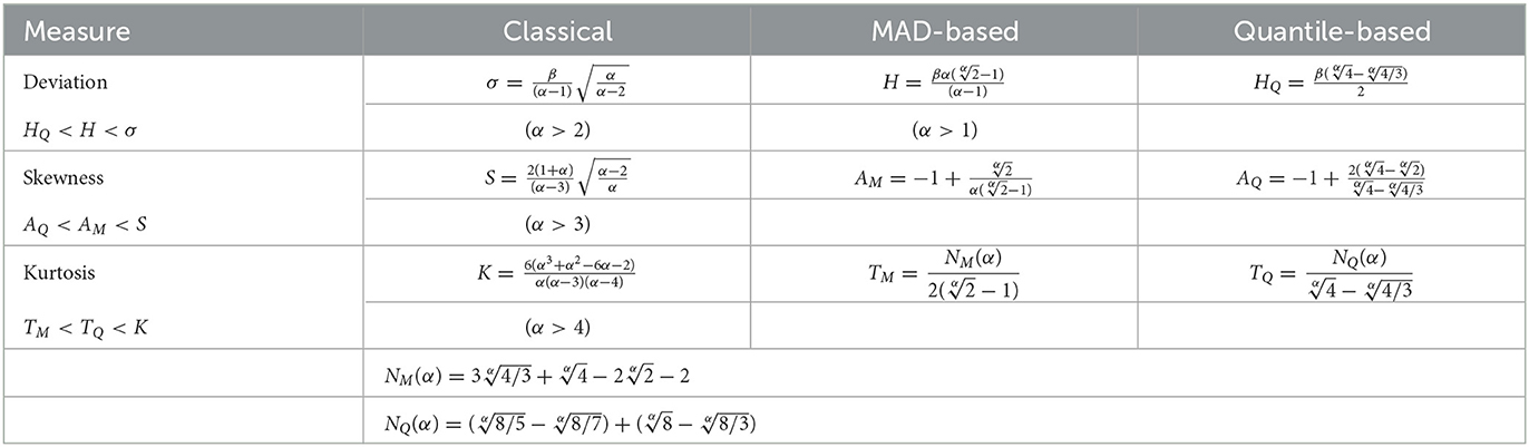
Table 6. A comparison of measures for Pareto distribution.

In Appendix (Section A4), we examined the asymptotic behavior of these measures for α ↦ 1 and for α ↦ ∞. For α ↦ 1, we showed that for MAD-based measures that H ↦ ∞, A_M ↦ 1, and T_M ↦ 1 whereas for quantile-based measures H_Q ↦ 4/3, A_Q ↦ 0.5, and T_Q ↦ 2.17. By contrast, for α ↦ ∞ we showed in Appendix (Section A4) that both MAD-based and quantile-based measures for skewness and kurtosis converge to the corresponding measures for exponential distribution H ↦ 0, A_M ↦ 0.44, T_M ↦ 0.62, H_Q ↦ 0, A_Q ↦ 0.26, T_Q ↦ 1.31 (see Table 4). Note that if X is Pareto with shape α and scale β, then Y = log(X/β) is exponentially distributed with rate α [20, 22].

9. Example: wealth distribution

Assume that income is distributed according to a Pareto principle p + q principle [20]: 100p% of all income is received by 100q% of people (p + q = 1) For example, the 60 − 40 rule (p = 0.6, q = 0.4) means that 40% of the people receive 60% of the wealth. We assume that p > 0.5.

This p + q principle with p > q corresponds to a Pareto distribution with a tail index α satisfying

$\alpha =\frac{log(p)}{log(p)-log(q)}$

For example, the 60 − 40 rule (p = 0.6, q = 0.4) has α = 2.260 whereas 80 − 20 rule (p = 0.8, q = 0.2) corresponds to α = log(5)/log(4)≈ = 1.161. If we take even larger p as in 95 − 5 rule (p = 0.95, q = 0.05 we get α = log(0.05)/log(0.95)≈1.017. It is easy to prove that ∂α/∂p < 0 and, therefore, α decreases as p increases. In particular, α↘1 as p ↦ 1. Larger values of p correspond to higher concentrations of wealth.

Figure 1 demonstrates that the MAD-based skewness approaches its asymptotic value of +1 more rapidly than the quantile-based skewness approaches its asymptotic value of 0.5. This behavior demonstrates that the MAD-based skewness A_M is better able to explore the extreme distribution of wealth and income in the highest brackets than using the quantile-based skewness.

FIGURE 1

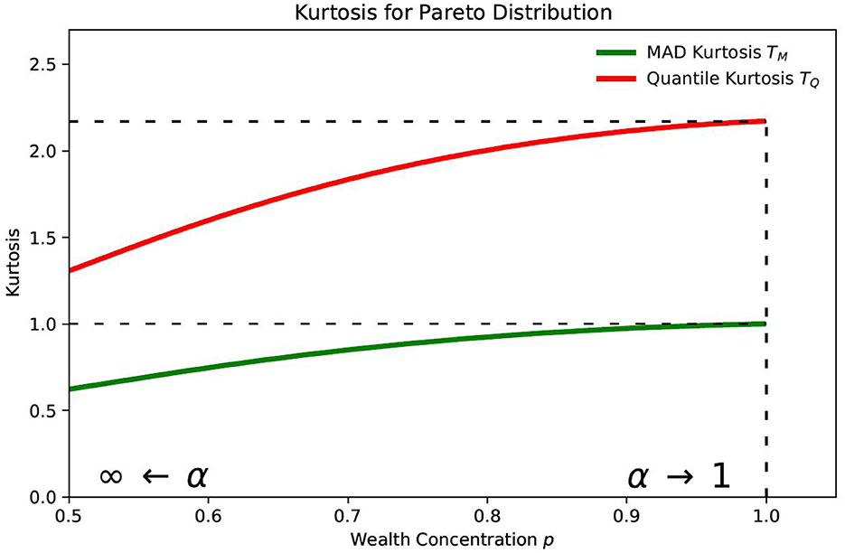
Figure 1. Skew for Pareto distribution.

It is important to note that in the case of α < 2, we cannot use classical measures for standard deviation, skewness, and kurtosis. By contrast, the MAD-based measures could be computed for these lower values of α and compared with the corresponding quantile-based measures.

As shown in Figure 2, the quantile-based kurtosis approaches its asymptotic value of 2.17 (from Equation A15 in Appendix) more rapidly than MAD-based kurtosis approaches its asymptotic value of 1. Despite this behavior in the kurtosis, we believe that skewness is more widely used and more revealing as a measure of the concentration of wealth and income at the highest brackets. The MAD-based kurtosis has the added practical advantage of having a maximum value of 1.

FIGURE 2

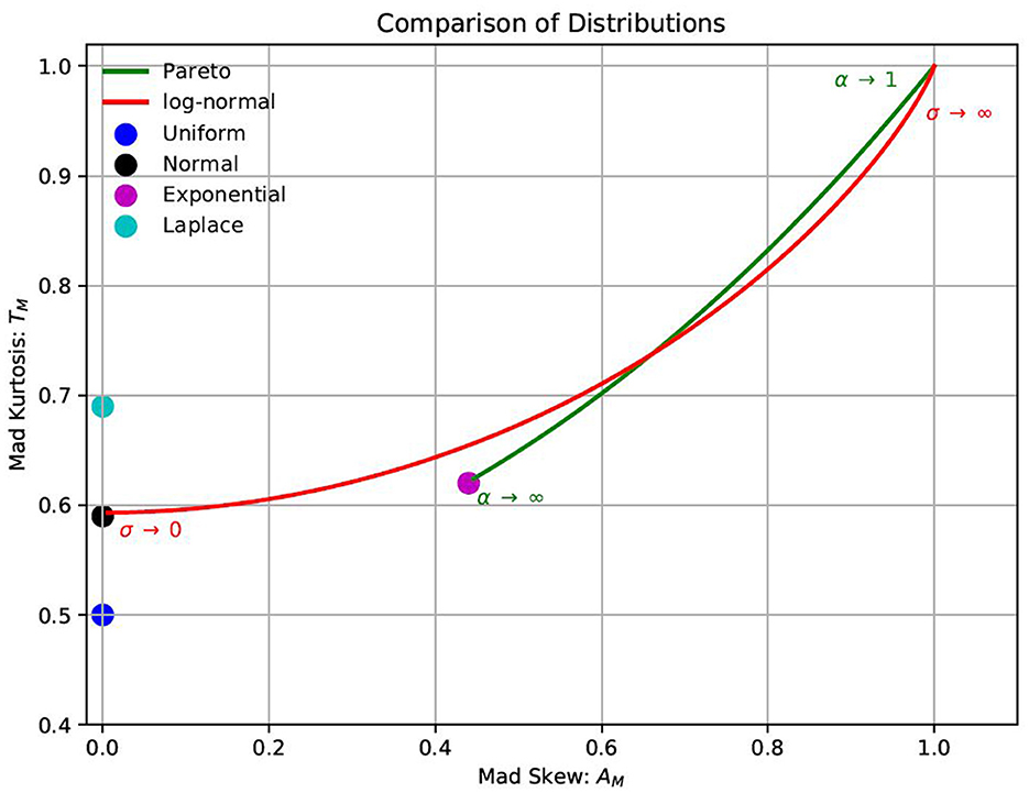
Figure 2. Kurtosis for Pareto distribution.

10. Comparison of distributions

Using MAD-based alternatives for deviation, skewness and kurtosis gives us additional ways to compare distributions. The MAD-based skewness A_M and MAD-based kurtosis T_M are always in the range −1 ≤ A_M ≤ 1 and 0 ≤ T_M ≤ 1, respectively. This is in contrast to classical and quantile-based measures that can be unbounded. Therefore, with MAD-based measures, we have a way to directly compare any two distributions in terms of their MAD-based skewness and kurtosis. In Figure 3, we plot both skewness and kurtosis for the distributions considered.

FIGURE 3

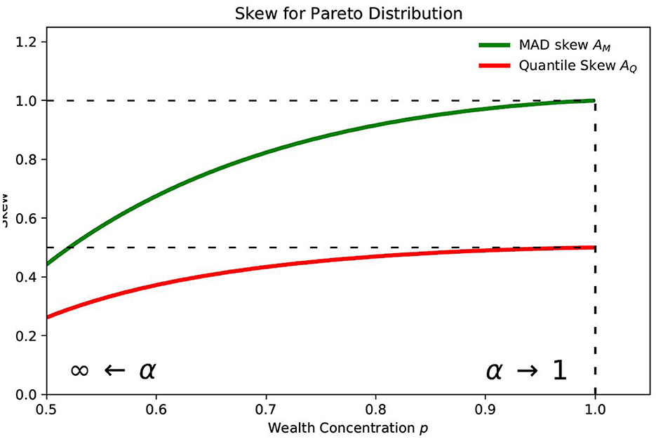
Figure 3. MAD-based skew/kurtosis comparison of distributions.

11. Conclusion

This paper considered MAD (about median)-based alternative metrics for classical standard deviation, skewness, and kurtosis. These MAD-based measures are shift-invariant. The MAD-based measures for skewness and kurtosis are also scale invariant. They can be computed from the corresponding left and right sub-ranges and require the existence of first-order moments only. The mathematical expressions for these measures are similar to those in quantile-based measures but involve computing means as opposed to quantiles. The resulting expressions can be interpreted as average values distance in sub-ranges from their respective medians.

In terms of practical applications, it is widely recognized that the median can be a better measure of centrality when the mean is overly influenced by outlier concentrations at the high end. The median captures the data centrality in many distributions with concentrations at the very high end, such as wealth and income. Building on the recognition that the median is the preferred metric in such applications, we go further in proposing MAD-based (about Median) metrics that give additional information and insight on the concentrations in the highest quantile.

For any distribution, the proposed MAD-based expressions for skewness and kurtosis are shown to be in the range [−1, 1] and [0, 1], respectively. The proposed MAD-based alternative measures provide a universal scale to compare skewness and kurtosis across different data sets.

Data availability statement

The original contributions presented in the study are included in the article/Supplementary material, further inquiries can be directed to the corresponding author.

Author contributions

SK proposed the initial idea and focused on examples and discussion. EP focused on analytical work. Both authors have read and approved the final manuscript.

Acknowledgments

The authors would like to thank Metropolitan College of Boston University and H. Chen School of Public Health of Harvard University for their support.

Conflict of interest

The authors declare that the research was conducted in the absence of any commercial or financial relationships that could be construed as a potential conflict of interest.

Publisher's note

All claims expressed in this article are solely those of the authors and do not necessarily represent those of their affiliated organizations, or those of the publisher, the editors and the reviewers. Any product that may be evaluated in this article, or claim that may be made by its manufacturer, is not guaranteed or endorsed by the publisher.

Supplementary material

The Supplementary Material for this article can be found online at: https://www.frontiersin.org/articles/10.3389/fams.2023.1206537/full#supplementary-material

References

1. Pham-Gia T, Hung TL. The mean and median absolute deviations. J Math Comput Modell. (2001) 34:921–36. doi: 10.1016/S0895-7177(01)00109-1

CrossRef Full Text | Google Scholar

2. Gorard S. Revisiting a 90-year-old debate: the advantages of the mean deviation. Brit J Educ Stud. (2005) 53:417–30. doi: 10.1111/j.1467-8527.2005.00304.x

CrossRef Full Text | Google Scholar

3. Farebrother RW. The historical development of the L₁ and L_∞ estimation methods. In: Dodge Y, editor. Statistical data Analysis Based on the L₁-norm and Related Topics. Amsterdam: North-Holland (1987). p. 37–63.

4. Portnoy S, Koenker R. The Gaussian hare and the Laplacian tortoise: computability of square-error versus abolute-error estimators. Stat Sci. (1997) 2:279–300.

5. Dodge Y. Statistical Data Analysis Based on the L₁ Norm and Related Topics. Amsterdam: North-Holland (1987).

Google Scholar

6. Elsayed KMT. Mean absolute deviation: analysis and applications. Int J Bus Stat Anal. (2015) 2:63–74. doi: 10.12785/ijbsa/020201

CrossRef Full Text | Google Scholar

7. Gorard S. An absolute deviation approach to assessing correlation. Brit J Educ Soc Behav Sci. (2015) 53:73–81. doi: 10.9734/BJESBS/2015/11381

CrossRef Full Text | Google Scholar

8. Gorard S. Introducing the mean deviation “effect” size. Int J Res Method Educ. (2015) 38:105–14. doi: 10.1080/1743727X.2014.920810

CrossRef Full Text | Google Scholar

9. Rousseeuw PJ, Croux C. Alternatives to the median absolute deviation. J Am Stat Assoc. (1993) 88:1273–83.

Google Scholar

10. Bloomfield P, Steiger WL. Least Absolute Deviations: Theory, Applications and Algorithms. Boston, MA: Birkhauser (1983).

Google Scholar

11. Shad SM. On the minimum property of the first absolute moment. Am Stat. (1969) 23:27.

Google Scholar

12. Schwertman NC, Gilks AJ, Cameron J. A simple noncalculus proof that the median minimizes the sum of the absolute deviations. Am Stat. (1990) 44:38–41.

Google Scholar

13. Upton G, Cook I. Understanding Statistics. Oxford: Oxford University Press (1996).

Google Scholar

14. Zwillinger D, Kokoska S. CRC Standard Probability and Statistics Tables and Formulae. New York, NY: CRC Press (2000).

Google Scholar

15. MacGillivray HI. Skewness and asymmetry. Ann Stat. (1986) 14:994–1011.

Google Scholar

16. Groeneveld RA, Meeden G. Measuring skewness and kurtosis. J R Stat Soc Ser D. (1984) 33:391–99.

Google Scholar

17. Habib E. Mean absolute deviation about median as a tool of exploratory data analysis. Int J Res Rev Appl Sci. (2012) 11:517–23.

Google Scholar

18. Bowley AL. Elements of Statistics. 4th ed. New York, NY: Charles Scribner (1920).

Google Scholar

19. Yule GU. An Introduction to the Theory of Statistics. London: C. Griffin, Limited (1912).

Google Scholar

20. Johnson NL, Kotz S. Distributions in Statistics. New York, NY: J. Wiley (1970).

21. Moors JJ. A quantile alternative to kurtosis. J R Stat Soc Ser D. (1988) 37:25–32.

Google Scholar

22. Feller JJ. Probability Theory and Applications. New York, NY: J. Wiley (1956).

Google Scholar

23. Huber PJ. Robust Statistics. New York, NY: J. Wiley (2009).

Google Scholar

24. Bennett N, Hays D, Sullivan B. The Wealth of Households: 2019. Washington, DC: Department of Commerce (2019). p. 1–6.

Google Scholar