Study of the stability of a meshless generalized finite difference scheme applied to the wave equation

1. Introduction

The wave equation is a well-known partial differential equation that is commonly used to model the behavior of a scalar function $u(\overrightarrow{r},t)$, where $\overrightarrow{r}$ denotes the spatial coordinates and t represents time. This scalar function can describe various physical phenomena, such as pressure waves on media or the displacement of particles from their equilibrium positions. The wave equation can be expressed as:

$\begin{array}{ll}\frac{{\partial }^{2}u}{\partial t^2}=c^2{\nabla }^{2}u,& (1)\end{array}$

c is a real non-zero coefficient representing wave propagation velocity, and ∇² denotes the spatial Laplacian operator.

Numerically solving the wave equation is a classical problem in partial differential equations, and many methods have been developed for this purpose. However, existing approaches often require rectangular or symmetrical regions, or involve a high computational cost.

Some finite-difference-based schemes have been developed recently to obtain numerical solutions to different partial differential equations. The main advantage of these schemes is their ability to achieve satisfactory results with low computational cost, making them relatively easy to implement. Some examples of such schemes can be found in [1–4].

After constructing a finite difference method, it is crucial to determine whether the scheme provides a stable approximation. Stability is essential for convergence, and several challenges arise in stability analysis when the scheme becomes more complex. Some authors have proposed bounds for specific problems. For instance, Alcrudo offered a practical selection of the temporal discretization Δt for the 2D scalar advection equation to ensure stability in [5]. This can be achieved by considering the inequality

$\Delta t\le {(\frac{a}{\Delta x}+\frac{b}{\Delta y})}^{-1},$

where Δx and Δy are the spatial discretizations, and a and b represent the advective velocities in the x and y directions, respectively.

For its part, other advances have been made in designing and applying finite difference schemes, including the corresponding stability analysis of these schemes. Appadu presents in [6, 7] different schemes to numerically solve the 1D advection-diffusion equation with very satisfactory results. In addition, the work presented in [8] shows a complete stability analysis, obtaining stability regions of each of the proposed methods.

Similar studies can be found for the wave equation. For instance, a proper selection for Δt is presented in [9] as

$\frac{c\Delta t}{h}\le \sqrt{\frac{a_1}{a_2}},$

where h is the grid size, a₁ is the sum of the absolute values of weights for the finite difference operators for ∂²u/∂t², and a₂ is the sum of the absolute values of weights for the finite difference operators for ∇²u. This bound ensures the production of stable results for the wave equation; however, as can be seen, it is limited to regular discretizations over a rectangle. Another remarkable example of the application of finite differences to obtain the numerical solution of the wave equation can be found in [10], where some CTCS schemes are presented for solving the 1+1D case, with great performance.

For the case of interest in this work, irregular 2D spatial domains (see Figure 1) are considered. Due to this, the classical bounds cannot be applied since the spatial discretizations are no longer a regular set of points on a grid.

FIGURE 1

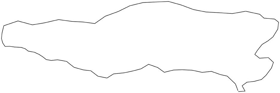
Figure 1. Irregular 2D region.

In this context, a generalized finite difference scheme is proposed in this paper, building upon the ideas presented in [11]. However, despite the utility of generalized finite differences, only some advances in stability analysis exist for these schemes. In previous works such as [12–15], the authors present stability analyses for generalized finite difference schemes applied to a modified Lax-Wendroff scheme for advection equation, and the pure advection, diffusion, and advection-diffusion equations. Given the importance of establishing stability conditions for the wave equation, this paper presents a Von-Neumann stability analysis for the proposed scheme.

2. Generalized finite differences applied to wave equation

The stability analysis presented in the following section arises from the problem of obtaining a finite-difference scheme for the wave equation problem over a simply connected planar domain Ω with a positively oriented Jordan polygon as its boundary. The problem is defined as:

$\begin{array}{ll}\begin{array}{lll}\frac{{\partial }^{2}u}{\partial t^2}=c^2(\frac{{\partial }^{2}u}{\partial x^2}+\frac{{\partial }^{2}u}{\partial y^2}),\hfill & \Omega \times [0,T],\hfill & c\in R,\hfill \end{array}& (2)\end{array}$

$\begin{array}{c}\begin{array}{ccc}\hfill u(x,y,0)=h(x,y,0),\hfill & (x,y)\in \Omega ,\hfill & \hfill \\ u(x,y,t){|}_{\partial \Omega }=h(x,y,t),\hfill & (x,y)\in \Omega ,\hfill & t\in [0,T],\hfill \end{array}\\ \begin{array}{lll}\frac{\partial u(x,y,0)}{\partial t}=g(x,y),\hfill & (x,y)\in \Omega .\hfill & \hfill \end{array}& (3)\end{array}$

In order to address this problem, first, the equation is partially discretized in time, followed by the discretization of the spatial derivatives. Both discretizations are presented in the following subsections.

2.1. Temporal discretization

The stability of the scheme for the wave equation relies heavily on the discretization of the second-order partial time derivative. To achieve this, it is possible to follow the steps provided below.

1. First, the time derivative can be expressed as its finite difference approximation. This is,

$\frac{{\partial }^{2}u(x,y,t)}{\partial t^2}\approx \frac{u_i^{k+1}-2u_i^k+u_i^{k-1}}{{(\Delta t)}^2},$

where $u_i^k$ stands for the approximation of u at the grid node p_i, at a time level k.

2. For an arbitrary node on the cloud, p₀ = (x₀, y₀), the equation can be written as

$\frac{u_0^{k+1}-2u_0^k+u_0^{k-1}}{{(\Delta t)}^2}=c^2(\frac{{\partial }^{2}u}{\partial x^2}+\frac{{\partial }^{2}u}{\partial y^2}),$

or, solving for $u_0^{k+1}$,

$\begin{array}{ll}{u}_0^{k+1}=2u_0^k-u_0^{k-1}+{(c\Delta t)}^2(\frac{{\partial }^{2}u}{\partial x^2}+\frac{{\partial }^{2}u}{\partial y^2}).& (4)\end{array}$

As seen, this approximation requires two different time steps to be computed. Due to this, it is essential to properly approximate the second time step.

3. It is possible to consider the condition for the first partial derivative in time

$\frac{\partial u(x,y,0)}{\partial t}=g(x,y),$

and apply central finite differences to get

$\frac{u_0^1-u_0^{-1}}{2\Delta t}=g(x,y),$

now, solving for $u_0^{-1}$, it can be rewritten as

$\begin{array}{ll}{u}_0^{-1}=u_0^1-2\Delta tg(x,y).& (5)\end{array}$

4. Let us assume that (4) holds at k = 0, this is,

$\begin{array}{ll}{u}_0^1=2u_0^0-u_0^{-1}+{(c\Delta t)}^2(\frac{{\partial }^{2}u}{\partial x^2}+\frac{{\partial }^{2}u}{\partial y^2}){|}_{t=0},& (6)\end{array}$

therefore, it is possible to replace (5) into (6) to obtain,

$\begin{array}{ll}{u}_0^1=u_0^0+\Delta tg(p_0)+\frac{{(c\Delta t)}^2}{2}(\frac{{\partial }^{2}u}{\partial x^2}+\frac{{\partial }^{2}u}{\partial y^2}){|}_{t=0,p_0}.& (7)\end{array}$

With this, the discretizations (4) and (7) can compute all the time steps required for the scheme.

2.2. Spatial discretization

Next, the spatial discretization is carried out for the partially discretized equation in time, which is accomplished using a generalized finite differences scheme.

To begin, a second-order linear operator

$Lu=A{u}_{xx}+B{u}_{xy}+C{u}_{yy}+D{u}_x+E{u}_y+Fu$

where A, B, C, D, E, and F are spatial functions specified by the operator, is considered. At a central node p₀ = (x₀, y₀), this operator can be approximated for a cloud points distribution, as illustrated in Figure 2, by using the values of u at nearby nodes p_i = (x_i, y_i), i = 1, 2, …, q, that are sufficiently close, which will be further discussed later in the manuscript.

FIGURE 2

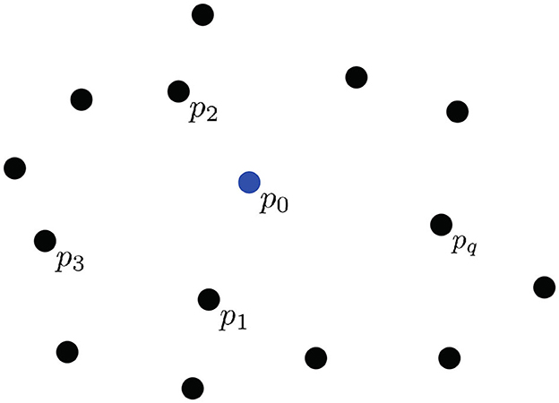
Figure 2. Arbitrary distribution of nodes.

A finite-difference scheme at the node p₀ can then be expressed as a linear combination

$L_0{u}_0={\Gamma }_{0}u(p_0)+{\Gamma }_{1}u(p_1)+\cdots +{\Gamma }_{q}u(p_q)={\displaystyle \sum _{i=0}^q}{\Gamma }_{i}u(p_i),$

where Γ₀, Γ₁, … , Γ_q are appropriate weights.

In [16, 17], it is stated that a finite difference scheme L₀ is consistent with the linear operator L if the local truncation error τ satisfies

$\begin{array}{ll}\tau ={\left[Lu\right]}_{p_0}-{\left[L_{0}u\right]}_{p_0}\to 0& (8)\end{array}$

when p₁, p₂, … , p_q→p₀.

The Taylor's series expansion of the consistency condition, up to the second order, yields

$\begin{array}{rr}{\left[Lu\right]}_{p_0}-{\left[L_{0}u\right]}_{p_0}& =\\ (F(p_0)-{\displaystyle \sum _{i=0}^q}{\Gamma }_i)u(p_0)+(D(p_0)-{\displaystyle \sum _{i=1}^q}{\Gamma }_i\Delta x_i)u_x(p_0)& +\\ (E(p_0)-{\displaystyle \sum _{i=1}^q}{\Gamma }_i\Delta y_i)u_y(p_0)+(A(p_0)-{\displaystyle \sum _{i=1}^q}\frac{{\Gamma }_i{(\Delta x_i)}^2}{2})u_{xx}(p_0)& +\\ (B(p_0)-{\displaystyle \sum _{i=1}^q}{\Gamma }_i\Delta x_i\Delta y_i)u_{xy}(p_0)+(C(p_0)-{\displaystyle \sum _{i=1}^q}\frac{{\Gamma }_i{(\Delta y_i)}^2}{2})u_{yy}(p_0)& +\\ O{(max\left\{\Delta x_i,\Delta y_i\right\})}^3\end{array}$

in this case, Δx_i = x_i−x₀ and Δy_i = y_i−y₀. Now, according to the consistency condition (8), it is required that

$\begin{array}{l}\begin{array}{c}A(p_0)-{\displaystyle \sum _{i=1}^q}\frac{{\Gamma }_i{(\Delta x_i)}^2}{2}=0,\\ B(p_0)-{\displaystyle \sum _{i=1}^q}{\Gamma }_i\Delta x_i\Delta y_i=0,\\ C(p_0)-{\displaystyle \sum _{i=1}^q}\frac{{\Gamma }_i{(\Delta y_i)}^2}{2}=0,\end{array}\begin{array}{c}D(p_0)-{\displaystyle \sum _{i=1}^q}{\Gamma }_i\Delta x_i=0,\\ E(p_0)-{\displaystyle \sum _{i=1}^q}{\Gamma }_i\Delta y_i=0,\\ F(p_0)-{\displaystyle \sum _{i=0}^q}{\Gamma }_i=0.\end{array}\end{array}$

These conditions define the linear system

$\begin{array}{ll}\left(\begin{array}{cccc}1& 1& \dots & 1\\ 0& \Delta x_1& \dots & \Delta x_q\\ 0& \Delta y_1& \dots & \Delta y_q\\ 0& {(\Delta x_1)}^2& \dots & {(\Delta x_q)}^2\\ 0& \Delta x_1\Delta y_1& \dots & \Delta x_q\Delta y_q\\ 0& {(\Delta y_1)}^2& \dots & {(\Delta y_q)}^2\end{array}\right)\left(\begin{array}{c}{\Gamma }_0\\ {\Gamma }_1\\ {\Gamma }_2\\ .\\ .\\ .\\ {\Gamma }_q\end{array}\right)=\left(\begin{array}{c}F(p_0)\\ D(p_0)\\ E(p_0)\\ 2A(p_0)\\ B(p_0)\\ 2C(p_0)\end{array}\right).& (9)\end{array}$

An important remark must be made, system (9) must be full-row-ranked to produce suitable approximations of the waves, and therefore, this fact must be taken into account for choosing the neighbors in the clouds.

Now, the scheme defined by (9) can be used to approximate the linear operator,

$Lu={(c\Delta t)}^2\left[\frac{{\partial }^{2}u}{\partial x^2}+\frac{{\partial }^{2}u}{\partial y^2}\right]$

at each time level, taking A = C = (cΔt)², and B = D = E = F = 0. The resulting Γ_i coefficients, with the time discretizations (4) and (7) define the Generalized Finite-Difference Schemes

$\begin{array}{ll}{u}_0^1=u_0^0+\Delta tg(p_0)+\frac{1}{2}{\displaystyle \sum _{i=0}^q}{\Gamma }_i{u}_i^0& (10)\end{array}$

and

$\begin{array}{ll}{u}_0^{k+1}=2u_0^k-u_0^{k-1}+{\displaystyle \sum _{i=0}^q}{\Gamma }_i{u}_i^k,& (11)\end{array}$

for the wave equation, where k represent the time level and $u_i^k$ is the approximation to the solution in the point p_i = (x_i, y_i) at time kΔt.

Equation (11) is the algebraic representation of an explicit scheme, following the idea presented on [18]; it is possible to extend this scheme, adding a parameter, λ, to involve two different time levels:

$\begin{array}{ll}{u}_0^{k+1}=2u_0^k-u_0^{k-1}+\lambda ({\displaystyle \sum _{i=0}^q}{\Gamma }_i{u}_i^k)+(1-\lambda )({\displaystyle \sum _{i=0}^q}{\Gamma }_i{u}_i^{k+1})& (12)\end{array}$

where λ can take values in [0, 1]. Particularly, for λ = 0.5, the scheme is a Crank-Nicolson-like scheme.

As mentioned earlier, a critical issue for this method is the number of neighbor nodes q used in the scheme. Extensive tests have shown that considering all the nodes in a space lower or equal to δ, where δ is the average node distance along the boundary, an average of 6 neighbors are chosen for each approximation. This is a significant reduction in the number of nodes compared with other schemes in the literature [19, 20]. Figure 3 shows an example of this selection.

FIGURE 3

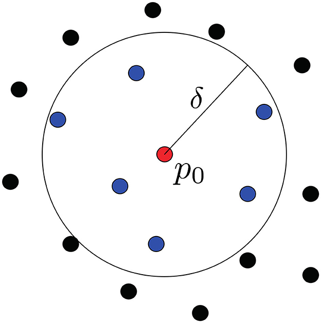
Figure 3. Selection of the neighbor nodes.

3. Stability analysis

Once the scheme is defined, a question that could naturally arise is whether the scheme produces a stable approximation since this is crucial to achieve convergence. Sousa illustrates in [21] the difficulties in stability analysis when the schemes become more complex, as is the case in clouds of points; taking this into account, in this section, analyses for the proposed schemes are presented to get theoretical bounds for the stability of the methods.

For the case of the explicit scheme (11),

$u_0^{k+1}=2u_0^k-u_0^{k-1}+{\displaystyle \sum _{i=0}^q}{\Gamma }_i{u}_i^k,$

following the Von-Neumann's stability analysis [22, 23], a generic component of the error at an arbitrary node p₀ = (x₀, y₀) at the k-th time-step could be measured as,

${\Phi }_0^k={\phi }^k{e}^{i(r{x}_0+s{y}_0)},$

where φ represents the amplification factor of the error. Since ${\Phi }_0^k$ satisfies the finite difference scheme, then,

$\begin{array}{r}{\phi }^{k+1}{e}^{i(r{x}_0+s{y}_0)}=2{\phi }^k{e}^{i(r{x}_0+s{y}_0)}-{\phi }^{k-1}{e}^{i(r{x}_0+s{y}_0)}+\\ {\displaystyle \sum _{l=0}^q}{\Gamma }_l{\phi }^k{e}^{i\left[r(x_0+\Delta x_l)+s(y_0+\Delta y_l)\right]},\end{array}$

so, in this case, φ must satisfy

$\begin{array}{r}{\phi }^{k+1}{e}^{i(r{x}_0+s{y}_0)}-2{\phi }^k{e}^{i(r{x}_0+s{y}_0)}+{\phi }^{k-1}{e}^{i(r{x}_0+s{y}_0)}=\\ {\displaystyle \sum _{l=0}^q}{\Gamma }_l{\phi }^k{e}^{i\left[r(x_0+\Delta x_l)+s(y_0+\Delta y_l)\right]}.\end{array}$

Then, the amplification factor satisfies

$\begin{array}{l}{\phi }^2-2\phi +1=\phi {\displaystyle \sum _{l=0}^q{\Gamma }_l}{e}^{i\left[r\Delta x_l+s\Delta y_l\right]}\\ =\phi {\displaystyle \sum _{l=0}^q{\Gamma }_l}[1+\left(r\Delta x_l-s\Delta y_l\right)i-\\ \frac{1}{2}\left(r^2\Delta x_l^2+2rs\Delta x_l\Delta y_l+s^2\Delta y^2\right)\\ +O{\left(\Delta x_l,\Delta y_l\right)}^3]\\ \approx \phi [{\displaystyle \sum _{l=0}^q{\Gamma }_l}+ir{\displaystyle \sum _{l=0}^q{\Gamma }_l}\Delta x_l+is{\displaystyle \sum _{l=0}^q{\Gamma }_l}\Delta y_l-\\ \frac{r^2}{2}{\displaystyle \sum _{l=0}^q{\Gamma }_l}\Delta x_l^2\\ -rs{\displaystyle \sum _{l=0}^q{\Gamma }_l}\Delta x_l\Delta y_l-\frac{s^2}{2}{\displaystyle \sum _{l=0}^q{\Gamma }_l}\Delta y_l^2].\end{array}$

By applying the consistency conditions up to the second order, it is possible to write

${\phi }^2-2\phi +1=-\Delta t^2{c}^2(r^2+s^2)\phi ,$

or

${\phi }^2-\alpha \phi +1=0,$

with α = 2−Δt²c²(r²+s²). Let us notice in this expression that α ≤ 2, and let us choose −2 ≤ α ≤ 2.

The solution of the quadratic equation can be expressed as

$\phi =\frac{\alpha \pm \sqrt{{\alpha }^2-4}}{2},$

in this case, since α² ≤ 4, then,

$|\phi {|}^2=1,$

and then, the scheme is conditionally stable.

Let us consider the case α² = 4; for this value, we get the bound

$\begin{array}{ll}\Delta t=\frac{2}{c\sqrt{r^2+s^2}}.& (13)\end{array}$

Following the same idea, for the implicit scheme (12),

$u_0^{k+1}=2u_0^k-u_0^{k-1}+\lambda ({\displaystyle \sum _{i=0}^q}{\Gamma }_i{u}_i^k)+(1-\lambda )({\displaystyle \sum _{i=0}^q}{\Gamma }_i{u}_i^{k+1}),$

where the error can be written as

$\begin{array}{l}{\phi }^{k+1}{e}^{i\left(r{x}_0+s{y}_0\right)}=2{\phi }^k{e}^{i\left(r{x}_0+s{y}_0\right)}-{\phi }^{k-1}{e}^{i\left(r{x}_0+s{y}_0\right)}\\ +\lambda \left({\displaystyle \sum _{l=0}^q{\Gamma }_l}{\phi }^k{e}^{i\left[r\left(x_0+\Delta x_l\right)+s\left(y_0+\Delta y_l\right)\right]}\right)\\ +(1-\lambda )\left({\displaystyle \sum _{l=0}^q{\Gamma }_l}{\phi }^{k+1}{e}^{i\left[r\left(x_0+\Delta x_l\right)+s\left(y_0+\Delta y_l\right)\right]}\right).\end{array}$

Then, the amplification factor satisfies

$\begin{array}{l}{\phi }^2-2\phi +1=\lambda \left(\phi {\displaystyle \sum _{l=0}^q{\Gamma }_l}{e}^{i\left[r\Delta x_l+s\Delta y_l\right]}\right)+(1-\lambda )\\ \left({\phi }^2{\displaystyle \sum _{l=0}^q{\Gamma }_l}{e}^{i\left[r\Delta x_l+s\Delta y_l\right]}\right)\\ =\lambda \phi {\displaystyle \sum _{l=0}^q{\Gamma }_l}[1+\left(r\Delta x_l-s\Delta y_l\right)i-\\ \frac{1}{2}\left(r^2\Delta x_l^2+2rs\Delta x_l\Delta y_l+s^2\Delta y^2\right)\\ -O{\left(\Delta x_l,\Delta y_l\right)}^3]+(1-\lambda ){\phi }^2\\ {\displaystyle \sum _{l=0}^q{\Gamma }_l}[1+\left(r\Delta x_l-s\Delta y_l\right)i\\ -\frac{1}{2}\left(r^2\Delta x_l^2+2rs\Delta x_l\Delta y_l+s^2\Delta y^2\right)-O{\left(\Delta x_l,\Delta y_l\right)}^3]\end{array}$

Once again, by applying the consistency conditions up to the second order,

${\phi }^2-2\phi +1=-\Delta t^2{c}^2(r^2+s^2)\lambda \phi -\Delta t^2{c}^2(r^2+s^2)(1-\lambda ){\phi }^2,$

now, considering

$\beta =\Delta t^2{c}^2(r^2+s^2),$

it is possible to write

${\phi }^2-2\phi +1=-\lambda \beta \phi -(1-\lambda )\beta {\phi }^2,$

this is,

$\left[1+(1-\lambda )\beta \right]{\phi }^2+(\lambda \beta -2)\phi +1=0,$

and, solving for φ,

$\begin{array}{l}\phi =\frac{-(\lambda \beta -2)\pm \sqrt{{(\lambda \beta -2)}^2-4\left(1+(1-\lambda )\beta \right)}}{2\left[1+(1-\lambda )\beta \right]}\\ =\frac{2-\lambda \beta \pm \sqrt{{\lambda }^2{\beta }^2-4\beta }}{2\left[1+(1-\lambda )\beta \right]},\end{array}$

now, considering λ²β ≤ 4, and using ∥·∥²,

$\begin{array}{l}\Vert \phi {\Vert }^2={\Vert \frac{2-\lambda \beta \pm \sqrt{{\lambda }^2{\beta }^2-4\beta }}{2\left[1+(1-\lambda )\beta \right]}\Vert }^2\\ =\frac{{(2-\lambda \beta )}^2-{\lambda }^2{\beta }^2+4\beta }{4{\left[1+(1-\lambda )\beta \right]}^2}\\ =\frac{1+\beta (1-\lambda )}{{\left[1+(1-\lambda )\beta \right]}^2}\\ =\frac{1}{1+(1-\lambda )\beta }\\ \le 1.\end{array}$

With this, in general, the implicit scheme turns out to be stable and, for the case λ = 0, it turns out to be unconditionally stable.

4. Numerical tests

To show the performance of the explicit and the implicit proposed schemes, four different regions were selected for the numerical tests: The unitary square [0, 1] × [0, 1], denoted as CUA, and three irregular, non-rectangular, non-symmetrical geometries designated as ENG, HAB, and PAT. Arbitrary clouds of points were generated for each region using an algorithm designed by Persson and Strang and presented in [24]. In Figure 4, it is possible to see one of the generated clouds of points for each region.

FIGURE 4

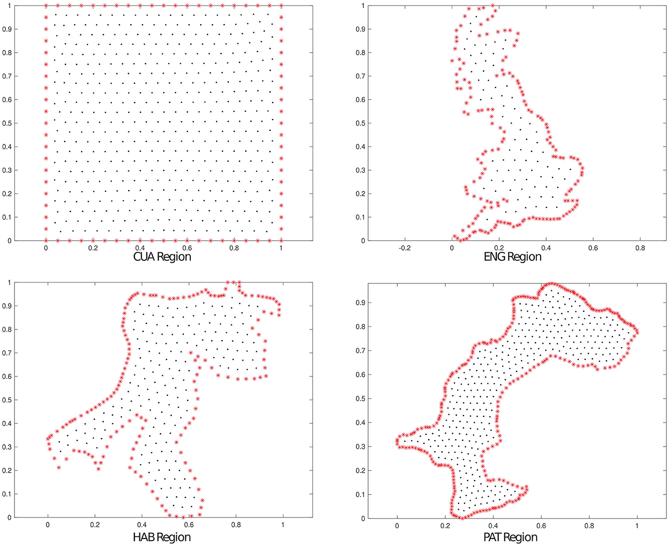
Figure 4. Clouds of points for the selected regions.

Two examples were solved for each region to show the method's accuracy. In both examples, the time interval [0, 1] was subdivided into 1, 000 subintervals, i.e., Δt = 0.001, to assure stability in most tests with the explicit scheme. Then, the norm of the quadratic error was computed as

$\Vert e{\Vert }_2^{(k)}=\sqrt{\frac{{\displaystyle {\sum }_i^n{(u_i^k-U_i^k)}^2}}{n}}$

where $U_i^k$ and $u_i^k$ are the approximated and theoretical solutions, respectively, at the i-th node and at a time k; and n is the total number of cloud nodes. Numerical solutions were computed for the explicit scheme (λ = 1) and implicit scheme with λ = 0.75, 0.50, 0.25, 0.00.

4.1. Example 1

Considering, as presented in [25], the equation

$2\frac{{\partial }^{2}u}{\partial t^2}-\frac{{\partial }^{2}u}{\partial x^2}-\frac{{\partial }^{2}u}{\partial y^2}=0,$

with initial conditions given by

$\begin{array}{ccc}u(x,y,0)=\sin (\pi (x+y)),& & \frac{\partial u}{\partial t}{\mid }_{t=0}=0,\end{array}$

and the following boundary condition

$u(x,y,t){\mid }_{\Omega }=cos(\pi t)sin(\pi (x+y))$

4.2. Example 2

For this second test, following the idea on [11], the equation

$\frac{{\partial }^{2}u}{\partial t^2}-\frac{{\partial }^{2}u}{\partial x^2}-\frac{{\partial }^{2}u}{\partial y^2}=0,$

is considered, with initial conditions given by

$\begin{array}{ccc}u(x,y,0)=\sin (\pi x)\sin (\pi y),& & \frac{\partial u}{\partial t}{\mid }_{t=0}=0,\end{array}$

and the boundary condition

$u(x,y,t){\mid }_{\Omega }=cos(\pi t\sqrt{2})sin(\pi x)sin(\pi y).$

Tables 1, 2 depict the error norms for the tests. Two different values of the error norm are considered in each case: in the first set of results, the mean of the error norm, over all time steps, is presented in order to show the overall performance of the schemes; in the second set of results, the error norm for the last time step is presented.

TABLE 1

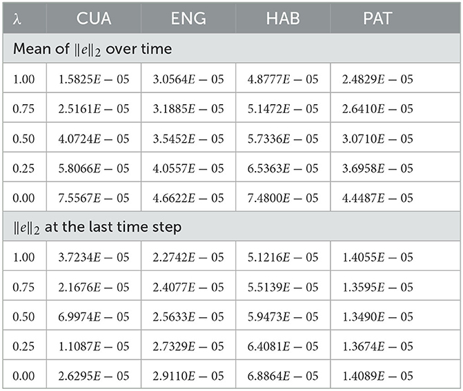
Table 1. Errors of Example 1 in all the clouds.

TABLE 2

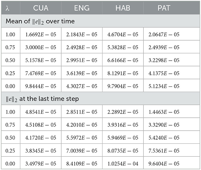
Table 2. Errors of Example 2 in all the clouds.

For the case of the implicit scheme, with λ = 0.75, Figures 5, 6 present a comparison between the numerical solution (on the left) and the theoretical solution (on the right) of the tests, in three different time levels for PAT region. It is possible to notice that both the approximated and the theoretical solutions present the same behavior.

FIGURE 5

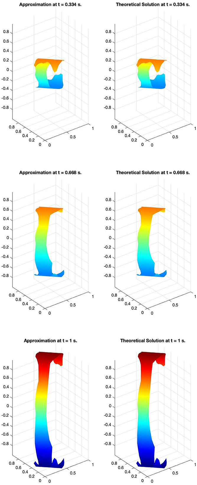
Figure 5. Numerical and Exact solutions for PAT at different time levels. Example 1.

FIGURE 6

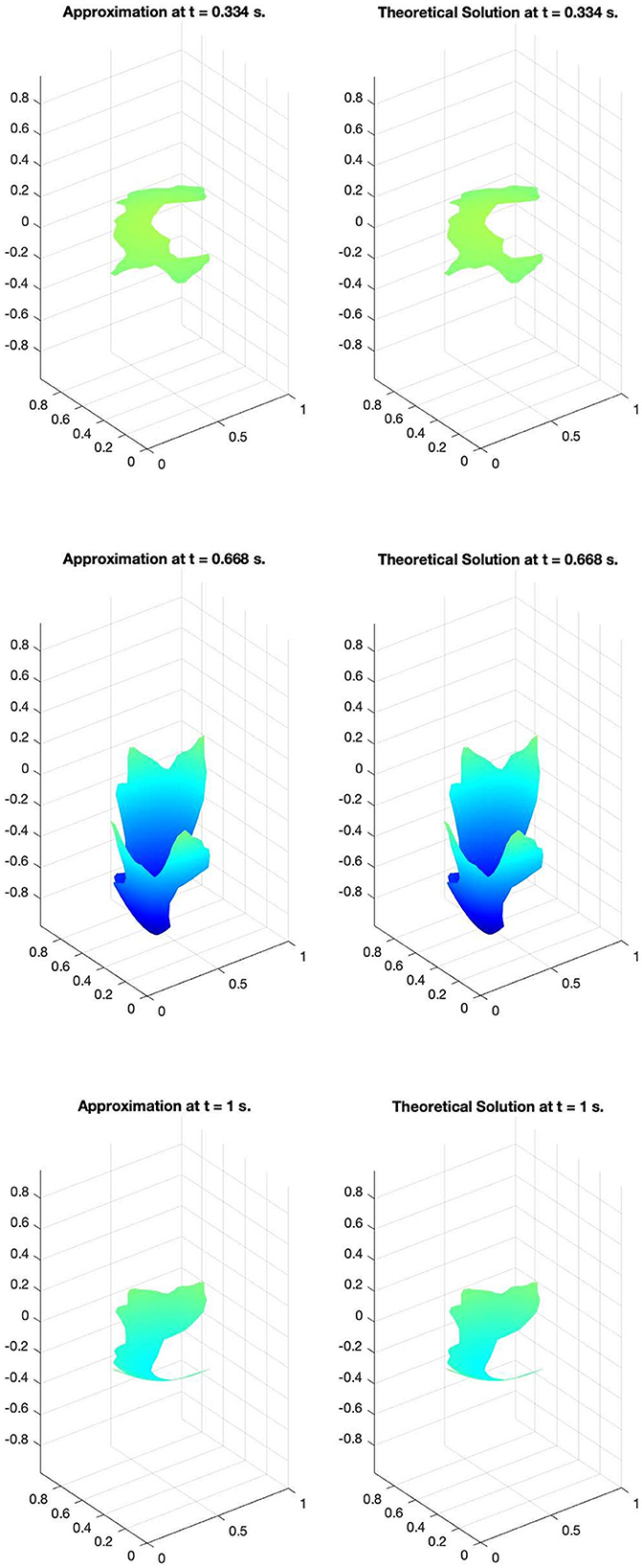
Figure 6. Numerical and Exact solutions for PAT at different time levels. Example 2.

The empirical convergence order of the method was estimated both for time and space. For the spatial case, the means of the quadratic error were calculated for clouds with a different number of nodes, for λ = 0. Denoting m as the total amount of nodes, Δ_m = 1/m, and e_Δm as the mean of the error computed then, given two pairs (e_Δi, Δ_i) and (e_Δj, Δ_j), the spatial empirical convergence order p_s was computed as

$p_s\approx \frac{log(\frac{\left|\right|e_{{\Delta }_i}\left|\right|}{\left|\right|e_{{\Delta }_j}\left|\right|})}{log(\frac{{\Delta }_i}{{\Delta }_j})},$

similarly, for the temporal convergence order, p_t , the computations were performed, denoting e_Δt as the error computed for the cloud using a Δ_t value. The results for these computations are reported in Table 3.

TABLE 3

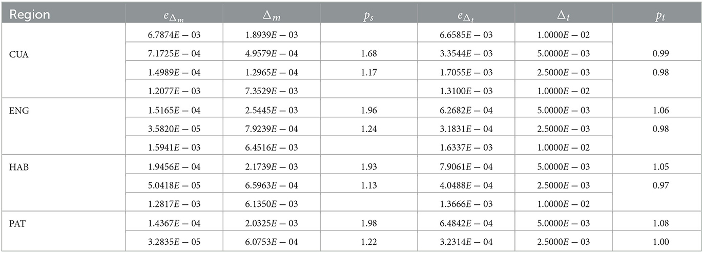
Table 3. Empirical spatial and temporal convergence orders.

The method implementation was developed in Python, and executed with Anaconda in Visual Studio Code. All tests were performed on an iMac (21.5-inch, Late 2013) with a 2.7 GHz quad-core Intel Core i5 processor and 8 GB of 1,600 MHz DDR3 RAM. The execution times, for all cases, were measured using the time library in Python, measuring the actual execution time instead of processor time. In the most time-consuming case, the execution took 3.015 s, while in the fastest case, it took 0.241 s.

Due to its stability, the implicit scheme can be applied to compute results for problems where there is no theoretical solution, even in non-simply-connected domains. In Figures 7, 8, it is possible to see the propagation of a wave, over CUA and HAB regions, with reflexive boundary conditions and a hole inside the region.

FIGURE 7

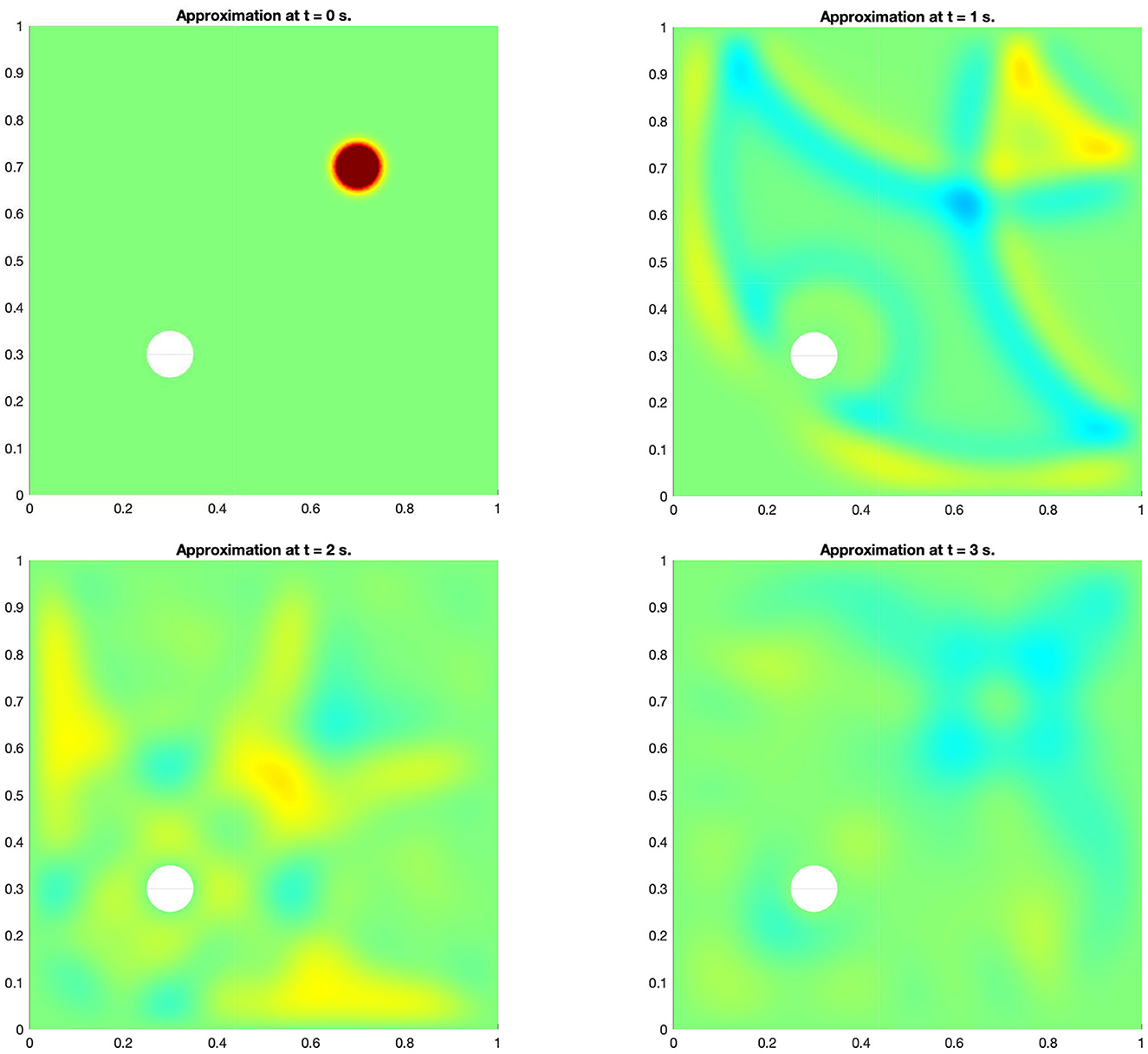
Figure 7. Computed wave propagation solution over CUA at different time levels.

FIGURE 8

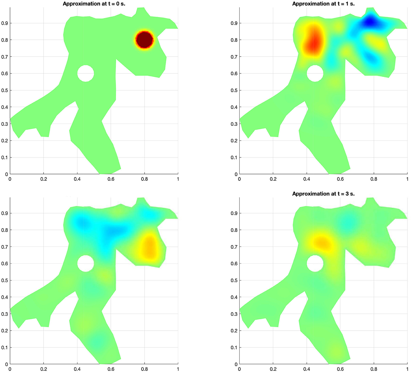
Figure 8. Computed wave propagation solution over HAB at different time levels.

5. Discussion and future work

In this work, two generalized finite differences schemes were presented to numerically solve the wave equation on highly irregular regions. Both schemes arise from the Taylor series expansion of the consistency condition introduced in [16, 17] for all finite difference schemes. The classical Lax-Richtmyer Equivalence Theorem [26] states that,

$\text{consistency}+\text{stability}\iff \text{convergence},$

since the proposed schemes arise from a consistency condition, stability is an important issue to study for a convergent scheme.

The presented Von-Neumann's stability analyses show that it is possible to obtain stability for both schemes; this agrees with the numerical results. For the case of the explicit scheme that turned out to be conditionally stable, it is possible to use the presented bound for Δt to get stable results. On the other hand, the implicit scheme proved to be unconditionally stable for the case of λ = 0, and no bound for Δt is required to compute stable results; even more, extensive tests have shown that with relatively big time-steps, it is possible to obtain stable results. Furthermore, the stability analyses were performed without considering any particular data structures. Due to this, they can be applied to all and every up-to-second-order finite difference scheme, not only to the ones presented in this work.

On the other hand, the numerical results show that the proposed schemes produce stable and accurate approximations of the exact solution of the wave equation, even in highly-irregular ones, such as HAB and PAT. The computed norms of the quadratic errors presented in this work show that the proposed schemes could be effective numerical methods to model different real-life scenarios involving the wave equation. And even more, the performed tests show that the results obtained are accurate without considering any weight functions, as in other methods.

A crucial issue to be remarked on is that the irregularity of the region needs to be considered since the number of nodes on the boundary needs to be enough to reproduce the area that is being studied correctly; due to this, a proper selection of the number of neighbor points and a correct choice of these might affect the accuracy when the region boundaries are highly irregular, and this has to be studied in the future.

Finally, it is worth highlighting the necessity of exploring the adaptability of the proposed methods to different physical problems governed by partial differential equations, such as shallow-water problems, where Robin boundary conditions are required to describe real-life phenomena.

Data availability statement

The original contributions presented in the study are included in the article/supplementary material, further inquiries can be directed to the corresponding author.

Author contributions

All authors listed have made a substantial, direct, and intellectual contribution to the work and approved it for publication.

Funding

Universidad Michoacana de San Nicolás de Hidalgo and CONACyT provide funds for open-access publication fees, and the International Center for Numerical Methods in Engineering provides technical and academic support.

Acknowledgments

The authors thank AULA CIMNE-Morelia, CIC UMSNH, and CONACyT for supporting this research.

Conflict of interest

The authors declare that the research was conducted in the absence of any commercial or financial relationships that could be construed as a potential conflict of interest.

Publisher's note

All claims expressed in this article are solely those of the authors and do not necessarily represent those of their affiliated organizations, or those of the publisher, the editors and the reviewers. Any product that may be evaluated in this article, or claim that may be made by its manufacturer, is not guaranteed or endorsed by the publisher.

References

1. Barrera-Sánchez P, Castellanos-Noda L, Domínguez-Mota FJ, González-Flores G, Pérez-Domínguez A. Adaptive discrete harmonic grid generation. Math Comput Simul. (2009) 79:1792–809. doi: 10.1016/j.matcom.2007.04.015

PubMed Abstract | CrossRef Full Text | Google Scholar

2. Domínguez-Mota FJ, Mendoza-Armenta S, Tinoco-Guerrero G, Tinoco-Ruiz JG. Numerical solution of poisson-Like equations with Robin boundary conditions using a finite difference scheme defined by an optimality condition. In: IMACS Series in Computational and Applied Mathematics: MASCOT 2011. Rome. (2012).

Google Scholar

3. Tinoco-Ruiz JG, Domínguez-Mota FJ, Mendoza-Armenta S, Tinoco-Guerrero G. Solving stokes equation in plane irregular region using an optimal consistent finite difference scheme. In: 20th International Meshing Roundtable. Paris. (2011).

Google Scholar

4. Tinoco-Ruiz JG, Domínguez-Mota FJ, Tinoco-Guerrero G, Fernández-Valdés PM, Mendoza-Armenta S. Numerical solution of differential equations in irregular plane regions using quality structured convex grids. Int J Model Simul Sci Comput. (2013) 4:1350004. doi: 10.1142/S1793962313500049

CrossRef Full Text | Google Scholar

5. Alcrudo F, García-Navarro P. A high-resolution Godunov-type scheme in finite volumes for the 2D shallow-water equations solution Godunov-type scheme in finite volumes for the 2D shallow-water equations. Int J Num Methods Fluids. (1993) 16:489–505.

Google Scholar

6. Appadu AR. Numerical solution of the 1D advection-diffusion equation using standard and nonstandard finite difference schemes. J Appl Math. (2013) 2013:734374. doi: 10.1155/2013/734374

CrossRef Full Text | Google Scholar

7. Appadu AR. Optimized composite finite difference schemes for atmospheric flow modeling. Num Methods Partial Diff Equat. (2019) 35:2171–92. doi: 10.1002/num.22407

CrossRef Full Text | Google Scholar

8. Appadu AR, Djoko JK, Gidey HH. A computational study of three numerical methods for some advection-diffusion problems. Appl Math Comput. (2016) 272:629–47. doi: 10.1016/j.amc.2015.03.101

CrossRef Full Text | Google Scholar

9. Lines LR, Slawinski R, Bording RP. A recipe for stability of finite-difference wave-equation computations. Geophysics. (1999) 64:967–9.

Google Scholar

10. Appadu AR, Waal GN. CTCS schemes for second order wave equation: numerical results and spectral analysis. Int J Eng Res Afr. (2021) 55:47–65. doi: 10.4028/www.scientific.net/JERA.55.47

CrossRef Full Text | Google Scholar

11. Tinoco-Guerrero G, Arias-Rojas H, Guzmán-Torres JA, Roman-Gutiérrez R, Tinoco-Ruiz JG. A meshless finite difference scheme applied to the numerical solution of wave equation in highly irregular space regions. Comput Math Appl. (2023) 126:25–33. doi: 10.1016/j.camwa.2023.01.035

CrossRef Full Text | Google Scholar

12. Tinoco-Guerrero G, Domínguez-Mota FJ, Gaona-Arias A, Ruiz-Zavala ML, Tinoco-Ruiz JG. A stability analysis for a generalized finite-difference scheme applied to the pure advection equation. Math Comput Simul. (2018) 147:293–300. doi: 10.1016/j.matcom.2017.06.001

CrossRef Full Text | Google Scholar

13. Tinoco-Guerrero G, Domínguez-Mota FJ, Tinoco-Ruiz JG. Stability aspects of a modified Lax-Wendroff scheme for irregular 2D regions. In: IMACS Series in Computational and Applied Mathematics: MASCOT 2015. Rome. (2015). p. 161–70.

Google Scholar

14. Tinoco-Guerrero G, Domínguez-Mota FJ, Tinoco-Ruiz JG. A study of the stability for a generalized finite-difference scheme applied to the advection-diffusion equation. Math Comput Simul. (2020) 176:301–11. doi: 10.1016/j.matcom.2020.01.020

CrossRef Full Text | Google Scholar

15. Tinoco-Ruiz JG, Domínguez-Mota FJ, Lucas-Martínez JS, Tinoco-Guerrero G. Study of the stability of a generalized finite difference scheme applied to the diffusion equation in irregular 2D space regions using convex grids. In: IMACS Series in Computational and Applied Mathematics: MASCOT 2018. Rome. (2019).

Google Scholar

16. Strikwerda JC.Finite Difference Schemes and Partial Differential Equations. Philadelphia, PA: Society for Industrial and Applied Mathematics (2004).

Google Scholar

17. Thomas JW. Numerical Partial Differential Equations: Finite Difference Methods. vol. 2 of Texts in Applied Mathematics. New York, NY: Springer (1995).

Google Scholar

18. Tinoco-Guerrero G, Domínguez-Mota FJ, Tinoco-Ruiz JG, Ruiz-Dí|az E. An implicit modified Lax-Wendroff scheme for irregular space 2D regions. In: IMACS Series in Computational and Applied Mathematics: MASCOT 2013. El Escorial. (2013). p. 18.

Google Scholar

19. Huang J, Fan CM, Chen JH, Yan J. Meshless generalized finite difference method for the propagation of nonlinear water waves under complex wave conditions. Mathematics. (2022) 10. doi: 10.3390/math10061007

CrossRef Full Text | Google Scholar

20. Salete E, Vargas AM, García A, Benito JJ, Ureña F, Ureña M. An effective numeric method for different formulations of the elastic wave propagation problem in isotropic medium. Appl Math Modell. (2021) 96:480–96. doi: 10.1016/j.apm.2021.03.015

CrossRef Full Text | Google Scholar

21. Sousa E. The controversial stability analysis. Appl Math Comput. (2003) 145:777–94. doi: 10.1016/S0096-3003(03)00274-1

CrossRef Full Text | Google Scholar

22. Grebenkov DS, Nguyen BT. Geometrical structure of Laplacian eigenfunctions. SIAM Rev. (2013) 55:601–67. doi: 10.1137/120880173

CrossRef Full Text | Google Scholar

23. Strauss WA. Chapter 8: Computations of Solutions. In:Rosatone L, Corliss S, , editors. Partial Differential Equations: An Introduction. 2nd ed. John Wiley & Sons (2009). p. 199–227.

Google Scholar

24. Persson PO, Strang G. A simple mesh generator in Matlab. SIAM Rev. (2004) 46:329–45. doi: 10.1137/S0036144503429121

PubMed Abstract | CrossRef Full Text | Google Scholar

25. Flores J, García A, Negreanu M, Salete E, Ureña F, Vargas AM. A spatio-temporal fully meshless method for hyperbolic PDEs. J Comput Appl Math. (2023) 2023:115194. doi: 10.1016/j.cam.2023.115194

CrossRef Full Text | Google Scholar

26. LeVeque RJ. Finite Difference Methods for Ordinary and Partial Differential Equations. Philadelphia, PA: Society for Industrial and Applied Mathematics (2007).

Google Scholar