Empirical examination of the Black–Scholes model: evidence from the United States stock market

1 Introduction

A derivative security is a contract for which the value is determined by the performance of an underlying security or collection of securities. The value is derived from the performance of assets, interest rates, currency exchange rates, or indices. Such securities can also be defined as financial instruments that do not constitute the ownership but rather a promise to convey ownership. The market for derivative securities has become huge in recent years. Worldwide, over-the-counter (OTC) derivative securities were worth a notional value of $632 trillion with a gross market value of $18.3 trillion at the end of June 2022 (1). Their economic function is to transfer the risk from those who do not want to bear it to those who are willing to bear it for a fee. In this respect, the derivatives market is much the same as the insurance industry. Due to their great flexibility, securities are traded by both professionals and retail investors. For these investors, equity derivatives such as warrants and options offer the opportunity to earn some extra income from their shares to protect the value of their existing shareholdings. Many applications are available to investors depending on the level of the risk they are willing to accept. Professional investors frequently use stock and index options to hedge their share portfolios. Index options allow investors to gain some broader exposure to the market compared with the single securities. Derivative contract types include options, swaps, futures, and forwards. This research focuses on the options contracts.

Options were firstly traded on an organized exchange in 1973, since when there has been dramatic growth in the market. An option is a contract between two parties in which one party has the right, but not the obligation, to buy or sell an underlying asset. Having rights without obligations has a financial value, so the option holders must purchase these rights, making them assets. These assets derive their values from some other asset, so they are called derivative assets. The two main types of options are call and put options. A call option is a right, but not an obligation, to buy an agreed quantity of a particular commodity or financial instrument (the underlying instrument) from the seller of the option at a specific time (the expiration date) for a certain price (the strike price). The seller (or writer) is obligated to sell the commodity or financial instrument, whereas the buyer has the right to buy or not buy. The buyer pays a fee called a premium for this right. The buyer of a call option hopes the price of the underlying instrument will rise in the future. If the buyer decides to exercise the option, the writer must sell the stock at the strike price. If the buyer does not exercise the option, the writer gains the premium. A put option is a contract between a seller and a buyer in which the seller has the right, but not the obligation, to sell a commodity or financial instrument to the writer of the option at a specific time for a certain price. The buyer of the put option hopes that the price of the stock will decrease and pay a premium. This premium cannot be returned, but simply provides the right to sell the stock at the strike price. Options contracts may be styled as either European or American. A European-style option can be exercised on the day of expiration, while an American-style option can be exercised at any time up to the day of expiration.

In 1973, the theoretical model for pricing European-style options was developed by Black and Scholes. This model has been widely used by many researchers, investors, and traders. The model is based on the following assumptions:

• The option is a European-style option (that is, the option can be exercised on the expiration date).

• There is continuous trading.

• Efficient markets (that is, the direction of the market cannot be predicted).

• The underlying stock does not pay dividends during the option’s life.

• There are no commissions or transaction costs for buying and selling options.

• The underlying assets’ risk-free interest rate and volatility are constant and known.

• The returns on the underlying stock are normally distributed.

• There are no riskless arbitrage opportunities.

The Black–Scholes formula takes the following variables into consideration:

• The current price of the underlying stock (S).

• Time until expiration (t), expressed as a percentage of a year.

• The volatility (σ) of the underlying stock.

• The strike price (K) of the option.

• The risk-free interest rate (r).

The Black–Scholes formulas are presented as follows.

The Call option premium

$C=S\varphi \left(d_1\right)-\varphi \left(d_2\right)K{e}^{-rt},$

The Put option premium

$P=\varphi \left(-d_2\right)K{e}^{-rt}-S\varphi \left(-d_1\right),$

where

$d_1=\frac{\ln \left(\frac{S}{K}\right)+\left(r+\frac{{\sigma }^2}{2}\right)t}{\sigma \sqrt{t}},$

$d_2=d_1-\sigma \sqrt{t},$

and $\varphi (.)$ is the cumulative standard normal distribution function.

2 Literature review

Black and Scholes (2) developed the Black–Scholes option pricing model (BSOPM) for European-style options. Although this model is widely used for pricing options contracts, its accuracy is subjected to debate. As a result, several studies have been conducted to test the model’s accuracy, and discrepancies have been found between the market value and the model value. Kumar and Agrawal (3) investigated the efficiency of the Black–Scholes model for the valuation of the call option contracts on eight stocks quoted on the National Stock Exchange of India (NSE). They compared the theoretical prices with the actual market price to examine the pricing accuracy, and observed that the Black–Scholes model mispriced options on several occasions and the volatilities were high for options that were highly overpriced. Sinha et al. (4) estimated the option premium of different call and put options by considering three different option chains from all mid-cap firms listed on the NSE. Their study showed that the option premium calculated using the Black–Scholes model was lower than the actual premium in the market, leaving the options overpriced. Srivastava and Shastri (5) examined whether the BSOPM is a good indicator of option pricing in the Indian context. The 10 most popular industry’s stocks listed on the NSE were considered. The BSOPM was applied considering both volatility and the risk-free rate. They applied a t-test to the hypothesis and determined the significance of the relationship between the BSOPM values and the actual values, and found that the BSOPM involves a significant degree of mispricing. Therefore, they concluded that the BSOPM alone cannot be adopted as an indicator of option pricing.

Several studies have compared the Black–Scholes model with other models to gage its accuracy. Yakoob (6) analyzed option valuation models (a modified Black–Scholes model with dividends, an absolute diffusion model, and the Hull–White stochastic volatility model) using options contracts on the S&P500 and S&P100 indexes. The option prices provided by various models were compared with the market prices of the options to evaluate the pricing accuracy, and the absolute and relative errors were computed. The Black–Scholes model was tested with both implied and historical volatility, and errors in the Black–Scholes formula were identified from analysis of the implied volatility smile. The absolute diffusion model, which assumes non-constant volatility, and the Hull–White stochastic volatility model, which assumes unpredictable random volatility, were found to provide far lower accuracy in pricing than the Black–Scholes model, particularly in the case of the Hull–White stochastic volatility model. Yakoob concluded that the Black–Scholes model is useful as an options valuation model and not simply a theorem. Yashwin et al. (7) analyzed the Black–Scholes model and Merton’s model to determine which is more applicable in India for European-style call options. They used both models to calculate the call option premium and compared the results with the actual call premium. The model giving the lowest percentage difference was considered to be favorable in predicting the call option premium. Under several assumptions, calculations, and interpretations, they concluded that Merton’s model is preferable. Swapna et al. (8) attempted to study the relevance of the Black–Scholes model and Black’s model in the Indian derivative market, with specific reference to banking stock options from the Nifty bank index. Their paired sample t-test revealed a significant difference between the model prices and market prices calculated through the Black–Scholes model. At the same time, no significant differences were observed between the calculated model prices and market prices of options under Black’s model. They observed that Black’s formula produces better alternatives than the Black–Scholes formula for pricing the banking stock call options.

There have been various suggestions regarding the assumptions of the Black–Scholes model. McKenzie et al. (9) evaluated the probability of an exchange-traded European call option exercised on the ASX200 option index using single-parameter estimates, which utilize qualitative regression and a maximum-likelihood approach. Their qualitative regression models indicated that the Black–Scholes model was significant at the 1% level in estimating the probability of an option being exercised. The results based on the maximum-likelihood method indicated that the factors of the Black–Scholes model are, collectively, statistically significant. That is, their test results showed that the Black–Scholes model is relatively accurate. The study of McKenzie et al. also provides evidence that the use of implied volatility and a jump-diffusion approach can increase the tail properties of the underlying lognormal distribution and improve the statistical significance of the Black–Scholes model. Krznaric (10) analyzed the price movement of 480 stocks in the S&P500 during the year 2014 to determine the effectiveness of the Black–Scholes formula for pricing call options. He found differences between the Black–Scholes prices and those of the actual stocks, and concluded that the model is not particularly accurate in pricing call options. Krznaric suggested that altering the market assumptions, especially those relating to constant volatility and known interest, could compensate for some of the limitations of the Black–Scholes model, and further said that the Black–Scholes method could be of value for identifying an option’s overall distribution over time, thus providing a reasonable starting point for pricing stock options. Huhta and Perttunen (11) evaluated the performance of the BSOPM on European call options written on the US S&P500 equity index in the year 2014. Their empirical results showed that strict assumptions related to the model must be relaxed to incorporate the observed market prices. They deduced that the assumptions about constant volatility and normally distributed error terms are incorrect and that the Black–Scholes model mispriced the US S&P500 index options in 2014. Arora and Sharma (12) investigated the efficiency of the option prices derived by the BSOPM using 10 stocks as samples for the determination of call and put option prices. The BSOPM seven-day moving average prices were used to compute the volatility. They found that theoretical option prices are mispriced when compared with the actual market option prices. Thus, they concluded that the BSOPM is not suitable for pricing option contracts and is not efficient for equity option pricing in the Indian market. They recommended that factors such as option volumes and implied volatility are mainly responsible for price changes in option contracts, rather than the five predictors considered in the BSOPM.

A number of modified Black–Scholes models have been used to compute more accurate option prices. For instance, Khan et al. (13) modified the Black–Scholes formula by adding new variables based on a given assumption related to the risk-free interest rate. They investigated the Black–Scholes model on the NSE derivative markets for European-style call (CE9000) and put (PE8500) options. Pearson’s correlation test was applied to compare the market value with both the modified and original Black–Scholes model. Their empirical results proved that the existing Black–Scholes model has a powerful effect that should not be neglected. Chauhan and Gor (14) compared a modified Black–Scholes model, which was obtained by changing the normal distribution to the truncated normal distribution, with the classical Black–Scholes model. They computed the theoretical prices for selected call options listed on the NSE, and concluded that the modified Black–Scholes model gave results that were closer to the market price of the options contracts.

To assess the efficiency of the Black–Scholes model, various studies have investigated different market periods. Angeli and Bonz (15) used the nonparametric Mann–Whitney U-test to examine whether the Black–Scholes model produces reasonable results during financially turbulent periods. They calculated the theoretical values of 5,814 options (3,366 put option price observations and 2,448 call option price observations) under the Black–Scholes assumptions, and compared them with the real market prices around the bankruptcy of Lehman Brothers. Their empirical results showed that, during this period of financial turbulences, the Black–Scholes model did not react sufficiently quickly to changes in market volatility. Both call and put options tended to be overpriced, but were more likely to be overpriced in the period after the Lehman Brothers collapse than before. They concluded that the Black–Scholes model performed differently in the period after Lehman Brothers went bankrupt than in the period before. Redroban and Cifuentes (16) examined the performance of the Black–Scholes formula before, during, and after two periods of market stress: the subprime crisis (October 2008) and the onset of the COVID-19 pandemic (March 2020). They found that the degree of mispricing was significant, exceeding 100% in many cases during both crises and in all scenarios analyzed. They concluded that the accuracy of the Black–Scholes formula is very poor.

3 Methodology

3.1 Research methodology

The classical BSOPM is for the non-dividend-paying assets and the European-style options. However, we will consider the extended Black–Scholes model, which was first introduced by Merton (17). The assumption that the pricing model can only be applied to European-style options is relaxed, allowing this model to be applied to American-style options. The extended Black–Scholes option pricing formulas with a dividend for call and put options at time t are described below.

$C_t=S_t{e}^{-\delta T}\varphi \left(d_1\right)-K{e}^{-rT}\varphi \left(d_2\right)$

$P_t=K{e}^{-rT}\varphi \left(-d_2\right)-S_t{e}^{-\delta T}\varphi \left(-d_1\right)$

where

$d_1=\frac{\ln \left(\frac{S_t}{K}\right)+\left(r-\delta +\frac{{\sigma }^2}{2}\right)T}{\sigma \sqrt{T}}$

$d_2=d_1-\sigma \sqrt{T}$

$S_t$ is the price of the underlying asset at time t, K is the strike price, δ is the dividend yield, σ is the volatility, T is the time until expiration, and $\varphi (.)$ is the cumulative standard normal distribution function.

This study uses the implied volatility calculated by Corrado and Miller’s model (18). According to Haug (19), the approximated implied volatility for a call option under Corrado and Miller’s model (18) is:

$\sigma \approx \frac{\sqrt{2\pi }}{S{e}^{\left(b-r\right)T}+K{e}^{-rT}}\left[\begin{array}{l}{c}_m-\frac{S{e}^{\left(b-r\right)T}-K{e}^{-rT}}{2}+\\ {\left[\begin{array}{l}{\left(c_m-\frac{S{e}^{\left(b-r\right)T}-K{e}^{-rT}}{2}\right)}^2-\\ \frac{{\left(S{e}^{\left(b-r\right)T}-K{e}^{-rT}\right)}^2}{\pi }\end{array}\right]}^{\frac{1}{2}}\end{array}\right]/\sqrt{T}$

where $c_m$is the market premium for the call option and b is the percentage cost of carrying the asset. The cost of carry b is interest rate minus the dividend yield. That is, b = r −  $\delta$ , and so b – r = − $\delta$ .

Hence, the implied volatility is estimated as:

$\sigma \approx \frac{\sqrt{2\pi }}{S{e}^{-\delta T}+K{e}^{-rT}}\left[\begin{array}{l}{c}_m-\frac{S{e}^{-\delta T}-K{e}^{-rT}}{2}+\\ {\left[\begin{array}{l}{\left(c_m-\frac{S{e}^{-\delta T}-K{e}^{-rT}}{2}\right)}^2-\\ \frac{{\left(S{e}^{-\delta T}-K{e}^{-rT}\right)}^2}{\pi }\end{array}\right]}^{\frac{1}{2}}\end{array}\right]/\sqrt{T}$

When ${\left(c_m-\frac{S{e}^{-\delta T}-K{e}^{-rT}}{2}\right)}^2-\frac{{\left(S{e}^{-\delta T}-K{e}^{-rT}\right)}^2}{\pi }$ < 0, Corrado and Miller’s approximation for implied volatility involves the square root of a negative number. Thus, in the formula, we replace the square root of a negative number with a value of 0; i.e., we use the square root from the formula as used by Chambers and Nawalkha (20). That is, if ${\left(c_m-\frac{S{e}^{-\delta T}-K{e}^{-rT}}{2}\right)}^2-\frac{{\left(S{e}^{-\delta T}-K{e}^{-rT}\right)}^2}{\pi }$ < 0, then ${\left[{\left(c_m-\frac{S{e}^{-\delta T}-K{e}^{-rT}}{2}\right)}^2-\frac{{\left(S{e}^{-\delta T}-K{e}^{-rT}\right)}^2}{\pi }\right]}^{\frac{1}{2}}$ would not have a real solution. For such cases, the implied volatility for the call option is calculated by:

$\sigma \approx \frac{\sqrt{2\pi }}{S{e}^{-\delta T}+K{e}^{-rT}}\left[c_m-\frac{S{e}^{-\delta T}-K{e}^{-rT}}{2}\right]/\sqrt{T}$

The implied volatility approximation for the put option is:

$\sigma \approx \frac{\sqrt{2\pi }}{S{e}^{-\delta T}+K{e}^{-rT}}\left[\begin{array}{l}{p}_m-\frac{\mathrm{}K{e}^{-rT}-S{e}^{-\delta T}}{2}+\\ {\left[\begin{array}{l}{\left(p_m-\frac{\mathrm{}K{e}^{-rT}-S{e}^{-\delta T}}{2}\right)}^2-\\ \frac{{\left(K{e}^{-rT}-S{e}^{-\delta T}\right)}^2}{\pi }\end{array}\right]}^{\frac{1}{2}}\end{array}\right]/\sqrt{T}$

where $p_m$is the market premium for a put option. The implied volatility does not have a real solution when ${\left(p_m-\frac{\mathrm{}K{e}^{-rT}-S{e}^{-\delta T}}{2}\right)}^2-\frac{{\left(K{e}^{-rT}-S{e}^{-\delta T}\right)}^2}{\pi }$  < 0. Thus, in the formula, the square root of a negative number is replaced by a value of 0; i.e., we use the square root from the formula as used by Chamber and Nawalkha (20). That is, if ${\left(p_m-\frac{\mathrm{}K{e}^{-rT}-S{e}^{-\delta T}}{2}\right)}^2-\frac{{\left(K{e}^{-rT}-S{e}^{-\delta T}\right)}^2}{\pi }$ < 0, then ${\left[{\left(p_m-\frac{\mathrm{}K{e}^{-rT}-S{e}^{-\delta T}}{2}\right)}^2-\frac{{\left(K{e}^{-rT}-S{e}^{-\delta T}\right)}^2}{\pi }\right]}^{\frac{1}{2}}$ would not have a real solution. For such cases, the implied volatility for a put option is calculated by:

$\sigma \approx \frac{\sqrt{2\pi }}{S{e}^{-\delta T}+K{e}^{-rT}}\left[p_m-\frac{\mathrm{}K{e}^{-rT}-S{e}^{-\delta T}}{2}\right]/\sqrt{T}$

3.2 Data

The data for the stock options chain were obtained from Yahoo Finance for May 17–June 17, 2022, for options expiring on July 24, 2022. The dividend yield was also obtained from Yahoo Finance. The companies considered in this study are the Bank of America (BAC), JPMorgan Chase & Co. (JPM), Wells Fargo & Company (WFC), Merck & Company, Inc. (MRK), Pfizer Inc. (PFE), UnitedHealth Group Incorporated (UNH), Apple Inc. (AAPL), Microsoft Corporation (MSFT), and NVIDIA Corporation (NVDA). We considered 252 trading days and took the 3-month rate from the United States Federal Reserve as the risk-free interest rate.

4 Empirical results

4.1 Stocks trend analysis

Figure 1 shows the trend in all stocks considered from May 17, 2022, to June 17, 2022. The closing price of stocks was used. According to the chart, all the stocks experienced a decline on May 17. Around May 18–19, the stocks started increasing till May 27, when it was relatively stable till June 7–9 and experienced a sharp decline afterward which could be a result of restrictive monetary policy to address the high inflation in the economy. However, WFC appears to experience fewer changes compared to other stocks.

Figure 1

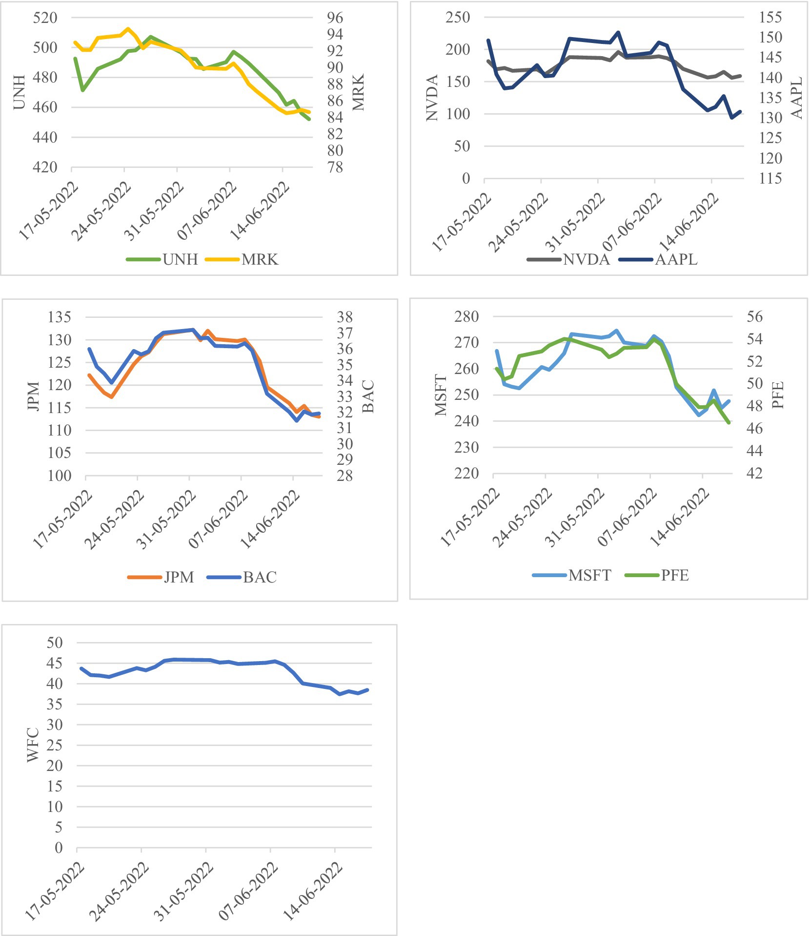
Figure 1. Trend in stock prices.

4.2 Paired sample t-test

A paired t-test is a parametric test, and all parametric tests depend upon the assumption of normality. Violation of the normality assumption does not cause a major problem for large sample sizes (greater than 30 or 40) (21). For sample sizes larger than 20, skewed data will still yield reliable test results, so the normality assumption can be waived for the samples of sufficient size (22). As our sample size for each stock was greater than 30, the normality assumption was not taken into consideration before performing the paired t-test.

The paired t-test compares the mean difference of the values with zero. For our study, the mean difference between the actual market premium and the Black–Scholes model premium is compared with zero. The null hypothesis and the alternative hypothesis are stated below.

Null hypothesis (H0): There is no significant difference between the actual market premium value and the Black–Scholes premium value.

Alternative hypothesis (H1): There is a significant difference between the actual market premium value and the Black–Scholes premium value.

The null hypothesis fails to be rejected at the 95% confidence level if the p value is greater than 0.05.

The paired sample t-test results for call options (Table 1) show no significant difference between the actual market premium and the Black–Scholes model premium for BAC, JPM, MRK, PFE, UNH, MSFT, and NVDA. There is a significant difference between the actual market premium and the Black–Scholes model premium for WFC and AAPL.

Table 1

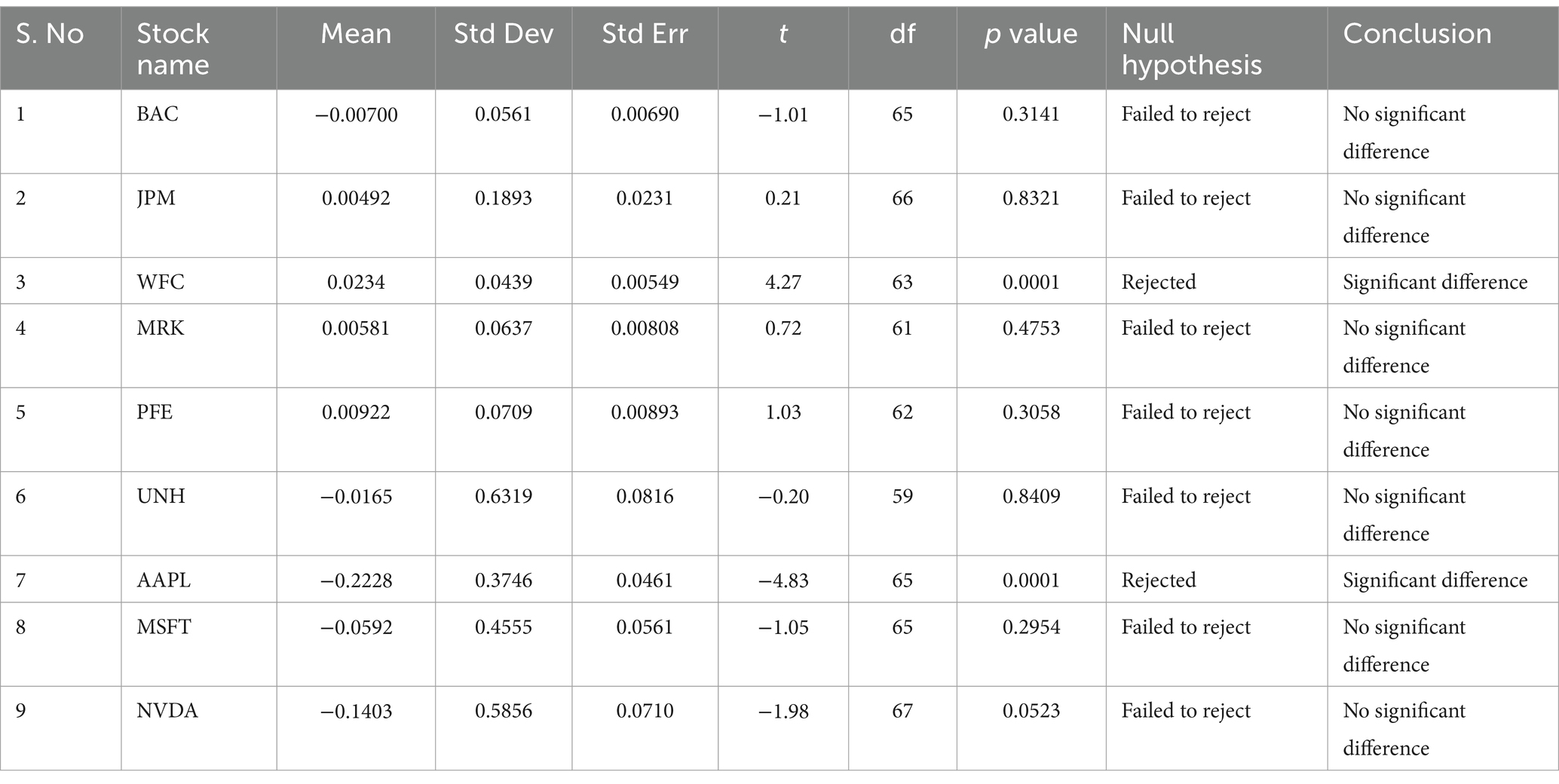
Table 1. Paired sample t-test for actual market premium value and Black–Scholes model premium value: call options.

From Table 2, the paired sample t-test results for put options indicate that there is no significant difference between the actual market premium and the Black–Scholes model for BAC, JPM, PFE, and NVDA. However, there is a significant difference between the actual market premium and the Black–Scholes model premium for WFC, MRK, UNH, AAPL, and MSFT.

Table 2

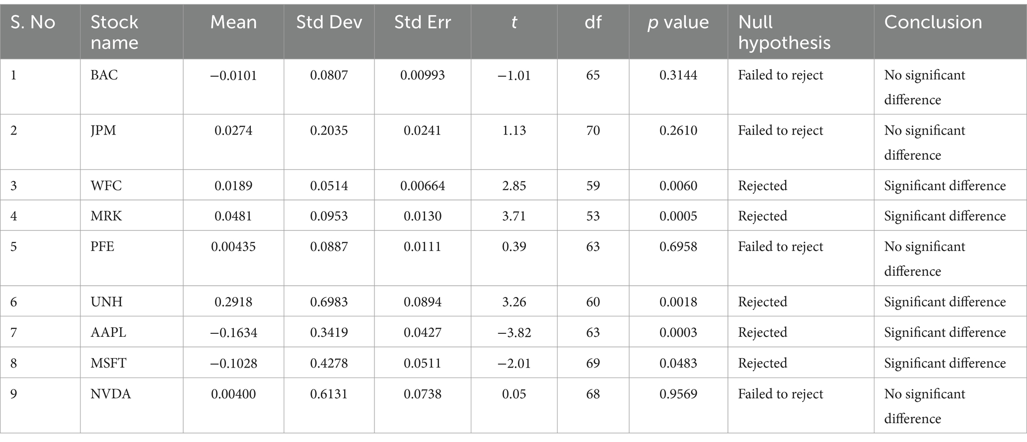
Table 2. Paired sample t-test for actual market premium value and Black–Scholes model premium value: put options.

For both call and put options (Tables 1, 2), WFC has the lowest standard deviation while UNH has the highest standard deviation. This implies that WFC has the least fluctuation and UNH has the highest fluctuation.

5 Discussion and conclusion

This research relaxed some of the Black–Scholes model assumptions to allow American-style options to be considered and examined the effectiveness of the BSOPM on selected stocks in the United States stock market. Empirical analysis was carried out using paired sample t-tests. The paired sample t-tests were applied to 582 call options and 579 put options. For the call options, the test results indicate no significant difference between the actual market premium value and the Black–Scholes model premium value for seven of the nine stocks considered. For put options, there is no significant difference between them for four out of the nine stocks. Hence, the BSOPM can be used to price call options in the United States stock market, but should not be used to price the put options.

The Black–Scholes model is relevant and can be used by investors to estimate the option price or premium. Like any commodities in financial markets, the option prices depend on supply and demand and are driven by many macro and micro indicators, such as GDP, inflation, interest rates, crude oil prices, exchange rates, per capita income, gold rates, and economic outlooks (5). Srivastava and Shastri (23) claimed that option prices depend on prevailing market conditions, such as predicted economic slumps, news related to a company, and a company’s performance and opportunities. Thus, a possible reason for the difference in the actual market and the Black–Scholes model premium for some of the stocks considered herein could be the high inflation rate in June 2022 in the United States. The Black–Scholes model could be modified to take market imperfections into consideration, or a new model for calculating option prices should be adopted. Further research should examine the effects of macro and micro economic indicators on the efficiency of the Black–Scholes model.

Data availability statement

Publicly available datasets were analyzed in this study. This data can be found here: https://docs.google.com/spreadsheets/d/1L561jCYKrsoPip2pZG1tgrOMr-vm_Tvm/edit?usp=sharing&ouid=102408132006705997753&rtpof=true&sd=true.

Author contributions

MS conducted all aspects of the research presented in this manuscript, including the study design, data collection, and manuscript writing. The manuscript was edited by Charlesworth Author Services to improve the grammar, syntax, and flow. The manuscript was also edited by Charlesworth Author Services to the journal style.

Acknowledgments

I would like to acknowledge Lakeshia Leggete Jones’s valuable contribution to my master’s dissertation at the University of Arkansas at Little Rock. Her detailed guidance has formed the basis for this research.

Conflict of interest

The author declares that the research was conducted in the absence of any commercial or financial relationships that could be construed as a potential conflict of interest.

Publisher's note

All claims expressed in this article are solely those of the authors and do not necessarily represent those of their affiliated organizations, or those of the publisher, the editors and the reviewers. Any product that may be evaluated in this article, or claim that may be made by its manufacturer, is not guaranteed or endorsed by the publisher.

Supplementary material

The Supplementary material for this article can be found online at: https://www.frontiersin.org/articles/10.3389/fams.2024.1216386/full#supplementary-material

References

1. Bank for International Settlements (2022). OTC Derivatives Statistics at end-June 2022. Available at: https://www.bis.org/publ/otc_hy2211.htm

Google Scholar

2. Black, F, and Scholes, M. The pricing of options and corporate liabilities. J Polit Econ. (1973) 81:637–54. doi: 10.1086/260062

Crossref Full Text | Google Scholar

3. Kumar, R, and Agrawal, R. An empirical investigation of the Black-Scholes call option pricing model with reference to NSE. Int J BRIC Bus Res. (2017) 6:01–11. doi: 10.14810/ijbbr.2017.6201

Crossref Full Text | Google Scholar

4. Sinha, A, Poonolly, J, and Gayathiri, A. Analysis of option prices using Black Scholes model. J Emerg Technol Innov Res. (2018) 5:12–21.

Google Scholar

5. Srivastava, A, and Shastri, M. A study of Black–Scholes Model’s applicability in Indian capital markets. Paradigm. (2020) 24:73–92. doi: 10.1177/0971890720914102

Crossref Full Text | Google Scholar

6. Yakoob, M. (2002). An empirical analysis of option valuation techniques using stock index options. Duke University Durham, NC. Available at: https://sites.duke.edu/djepapers/files/2016/08/yakoob.pdf

Google Scholar

7. Yashwin, BR, Chathurya, AM, and Thangjam, R. The practical applicability of Black Scholes model and Merton’s model on option pricing in India. J Emerg Technol Innov Res. (2018) 5:94–101.

Google Scholar

8. Swapna, HR, Arpana, D, and Geetha, R. An empirical study on pricing of options in Indian derivative market: with specific reference to private sector banks. Int J Disast Recov Bus Contin. (2020) 11:1347–56.

Google Scholar

9. McKenzie, S, Gerace, D, and Subedar, Z. An empirical investigation of the Black-Scholes model: evidence from the Australian stock exchange. Australas Acc Bus Fin J. (2007) 1:71–82. doi: 10.14453/aabfj.v1i4.5

Crossref Full Text | Google Scholar

10. Krznaric, M. (2016). Comparison of option price from Black-Scholes model to actual values. Williams Honors College, Honors Research Projects. Available at: http://ideaexchange.uakron.edu/honors_research_projects/396?utm_source=ideaexchange.uakron.edu%2Fhonors_research_projects%2F396&utm_medium=PDF&utm_campaign=PDFCoverPages

Google Scholar

11. Huhta, T, and Perttunen, J (2017). Performance of the Black-Scholes option pricing model—Empirical evidence on S&P500 call options in 2014. University of Oulu—Oulu Business School. Available at: http://jultika.oulu.fi/files/nbnfioulu-201711083066.pdf

Google Scholar

12. Arora, K, and Sharma, M. Empirical study on pricing efficiency of Black Scholes model of option pricing with special reference to equity options in India. Res Guru Online J Multidiscip Sub. (2019) 12:471–8.

Google Scholar

13. Khan, M, Gupta, A, and Siraj, S. Empirical testing of modified Black-Scholes option pricing model formula on NSE derivative market in India. Int J Econ Financ Issues. (2013) 3:87–98.

Google Scholar

14. Chauhan, A, and Gor, R. A comparative study of modified Black-Scholes option pricing formula for selected Indian call options. IOSR J Math. (2020) 16:16–22. doi: 10.9790/5728-1605011622

Crossref Full Text | Google Scholar

15. Angeli, A, and Bonz, C (2010). Changes in the creditability of the Black-Scholes option pricing model due to financial turbulences. Master’s thesis. Umea School of Business and Economics. 1–57. Available at: https://www.diva-portal.org/smash/get/diva2:326341/FULLTEXT01.pdf

Google Scholar

16. Redroban, S, and Cifuentes, A. On the performance of the Black and Scholes (B-S) options pricing formulas during the subprime and Covid-19 crises. Centro UC CLAPES UC. (2021) 32:75–85. doi: 10.1002/jcaf.22504

Crossref Full Text | Google Scholar

17. Merton, RC . Theory of rational option pricing. Bell J Econ Manag Sci. (1973) 4:141–83. doi: 10.2307/3003143

Crossref Full Text | Google Scholar

18. Corrado, CJ, and Miller, TW. A note on a simple, accurate formula to compute implied standard deviations. J Bank Financ. (1996) 20:595–603. doi: 10.1016/0378-4266(95)00014-3

Crossref Full Text | Google Scholar

19. Haug, EG . The Complete Guide to Option Pricing Formulas McGraw-Hill (2007).

Google Scholar

20. Chambers, DR, and Nawalkha, SK. An improved approach to computing implied volatility. Fin Rev. (2001) 36:89–100. doi: 10.1111/j.1540-6288.2001.tb00021.x

Crossref Full Text | Google Scholar

21. Ghasemi, A, and Zahediasl, S. Normality tests for statistical analysis: a guide for non-statisticians. Int J Endocrinol Metabol. (2012) 10:486–9. doi: 10.5812/ijem.3505

PubMed Abstract | Crossref Full Text | Google Scholar

22. Frost, J . Hypothesis Testing: An Intuitive Guide for Making Data Driven Decisions. State College, Pennsylvania: Statistics by Jim Publishing (2020).

Google Scholar

23. Srivastava, A, and Shastri, M. A study of relevance of Black-Scholes model on option prices of Indian stock market. Int J Govern Fin Intermediat. (2018) 1:82–104. doi: 10.1504/IJGFI.2018.091495

Crossref Full Text | Google Scholar

24. Muthusamy, A, and Vevek, S. Testing volatility for selected Indian indices. Pac Bus Rev Int. (2016) 8:35–42.

Google Scholar

25. Ray, S . A close look into Black-Scholes option pricing model. J Sci. (2012) 2:172–8.

Google Scholar

26. Macbeth, JD, and Merville, LJ. An empirical examination of the Black-Scholes call option pricing model. J Financ. (1979) 34:1173–86. doi: 10.2307/2327242

Crossref Full Text | Google Scholar

27. Black, F, and Scholes, M. The valuation of option contracts and a test of market efficiency. J Financ. (1972) 27:399–417. doi: 10.2307/2978484

Crossref Full Text | Google Scholar

28. Chauhan, A, and Gor, R. Black-Scholes option pricing model and its relevancy in Indian options market: a review. IOSR J Econom Fin. (2021) 12:1–7. doi: 10.9790/5933-1201020107

Crossref Full Text | Google Scholar

29. Solbakke, C, and Egly, H (2022). Implied and historical volatility—an empirical study on their predictive power of the future volatility on the OMXS30 index. Örebro University, School of Business. Available at: https://www.diva-portal.org/smash/get/diva2:1678397/FULLTEXT01.pdf

Google Scholar

30. Al Saedi, YH, and Tularam, GA. A review of the recent advances made in the Black-Scholes models and respective solutions methods. J Math Stat. (2018) 14:29–39. doi: 10.3844/jmssp.2018.29.39

Crossref Full Text | Google Scholar

31. Black, F . Fact and fantasy in the use of options. Financ Anal J. (1975) 31:36–41. doi: 10.2469/faj.v31.n4.36

Crossref Full Text | Google Scholar

32. Roll, R . An analytic valuation formula for unprotected American call options on stocks with known dividends. J Financ Econ. (1977) 5:251–8. doi: 10.1016/0304-405x(77)90021-6

Crossref Full Text | Google Scholar

33. Hull, J . Options, Futures, and Other Derivatives. Boston: Pearson Education Limited (2018).

Google Scholar

34. Federal Reserve (n.d.). FRB H15: Selected Interest Rate. Available at: https://www.federalreserve.gov/datadownload/Choose.aspx?rel=H15

Google Scholar

35. Yahoo! Finance (n.d.). Yahoo Finance—Business Finance, Stock Market, Quotes, News. Available at: https://finance.yahoo.com/

Google Scholar