Computing formation enthalpies through an explainable machine learning method: the case of lanthanide orthophosphates solid solutions

1 Introduction

In recent years, the role of existing Machine Learning (ML) methods has experienced a tremendous growth in many scientific computing domains including Materials Science and Quantum Chemistry [1–3]. Concurrently, new revolutionary methods and algorithms have appeared that expanded the range of applicability of existing state-of-the art techniques [4, 5]. This trend led to a high interest in general ML applications, which, in turn, left the scientific community, struggling in reconciling the need of developing refined tools with the assessment of their usefulness when applied to specific problems [6]. The assessment of their efficacy is particularly relevant when the target is an explainable learning method [7], and the domain knowledge is integrated in the final model [8].

In recent years, several machine learning methods have been proposed to predict enthalpies of formation of several categories of materials [9–11]. Despite their progress, none of these efforts provide a fully explainable model which outputs a mathematical expression, building on existing knowledge and improves it by adding additional terms that are statistically inferred.

In this article, we propose a three-step approach to use traditional machine learning tools to arrive at a scientifically consistent explainable method [7]. At first, we propose the use of Kernel Ridge Regression [12] methods to first assess which, out of a number of different kernels, provides the most reliable and transparent method. Second, we make a post-hoc interpretation of the model, and we proceed to reverse engineer it so as to find which coefficients of the model are the most relevant to recover a fully explainable mathematical expression for the target property. Finally, we integrate domain-specific knowledge by forcing scientific consistency through a constraint on how the input variables could be combined. The end result is a mathematical expression which relates the target property to the input variables in a functional dependence that replicates known results and add further terms, substantially improving the accuracy of the final expression.

Our methodology is, in part, inspired by the study by Ghiringhelli et al. [13, 14], which uses the Least Absolute Shrinkage and Selection Operator (LASSO) [15] together with a sparsification process they term LASSO+ℓ₀, to learn the most relevant descriptors for a given target property. In this study, we go beyond their approach by constraining the functional form of the prior using knowledge coming from both the algorithmic model (the assessment of best kernel) and integration of domain-knowledge (to ensure scientific consistency). To demonstrate the feasibility of our approach, we applied it to the specific problem of computing the excess enthalpy of formation of solid solution (enthalpy of mixing) of lanthanide orthophosphates (LnPO₄). We investigate the functional dependence of the mixing enthalpy for binary solid solutions of two distinct lanthanide cations (Ln), taking into account two distinct phases these materials form: monazite and xenotime [16].

1.1 Excess enthalpy of solid solution formation

Monazite is a phosphate mineral that contains rare-earth elements. Among these, lanthanide phosphates (LnPO₄) are the most widely distributed. These form monazite-type structure for Ln = La, …,Tb and xenotime-type (zircon) structure for heavier lanthanides [17–20]. Among other potential applications, synthetic (monazite-type) ceramic solid matrices are suitable for the conditioning of long-lived radionuclides, such as minor actinides (Np, Am, Cm) or Pu in the form of a synrock [21–23]. However, before these ceramics could be used in nuclear waste management, their physical and chemical properties and, most importantly, thermodynamic parameters have to be well-characterized and understood.

A solid solution is formed when two or more cations are incorporated into a solid host matrix on the same crystallographic site. When atoms of the solute solid phase are incorporated into the solvent solid host phase, the whole process can be interpreted as a sort of impurity inclusion into the host phase [24, 25]. Here, we consider a combination of two cations within a single phase, either monazite or xenotime. In reality, however, when lighter (monazite as stable structure) and heavier (xenotime as stable structure) lanthanide are mixed, such a solid solution has a wide miscibility gap, i.e., it is thermodynamically unstable in a wide solid solution range, with different stable phases of solid solution endmembers (solute and solvent). In these cases, the mixing enthalpy of single-phase solid solutions is a key factor for describing the two-phase cases, such as monazite-xenotime system [16, 26]. The excess enthalpy is a very important parameter that allows, for instance, for the estimation of solubility limits in mixed element systems. Accurate models for the excess enthalpy of mixing allow for the conversion of the concentrations of different lathanide elements measured in rocks, containing monazite and xenotime, to temperature-pressure conditions at which a given rock was formed [26]. Similar considerations were recently used to understand the maximum solubility limit of Fe in NiOOH-based electrocatalyst and the role of Fe in enhancing the oxygen evolution reaction (OER) activity—a key process considered for mass production of hydrogen as the fuel of the future green economy [27].

Whether a single phase solution will stay stable or not, the result is driven by the excess enthalpy of the mixing [24, 28]. The latter is defined as the difference between the formation enthalpies of the mixed compounds and those of the solid solution endmembers, which could be measured [29] or accurately computed [30–32]. The single phase solid solutions, such as monazite-type, resemble closely a symmetric solid solutions and are well-described by a simple model, H^E = m(1 − m)W, with W being the Margules interaction parameter and m the solid solution ratio [28, 33]. With systematic Density Functional Theory (DFT)-based calculations, it was found that for the monazite-type solid solutions, the Margules interaction parameter W is a function of the Young's modulus, Y, the unit-cell volume, V, and the unit-cell volume difference between the solid solution endmembers (solid and solute), ΔV, [34, 35]

$\begin{array}{ll}W~\frac{0.154Y}{V}\Delta V^2~\frac{Y}{6V}\Delta V^2.& (1)\end{array}$

The relationship between the excess formation of mixing and the physical parameters has been a topic of discussion of various studies [26, 28, 34]. Among these, the ionic radius R of the mixing cations is often used as the main discriminant parameter [26]. Such a choice, however, makes the thermodynamic parameters of the mixing only weakly material dependent. As such, the excess enthalpy of mixing of monazite-type and xenotime-type solid solutions is described with very similar relationship as a function of ΔR/R (Figure 6 of [26]).

In Figure 1, we illustrate how existing models describe the functional dependence on physical parameters of the excess of enthalpy for the data used in this study. Plot (a) shows the case of monazite for which the models of [34, 36] reproduce the data reasonably well. This is in part because both models use the difference in volumes of the endmembers as a parametric variable, while the model of the study mentioned in [26] uses the difference in ionic radii.

Figure 1

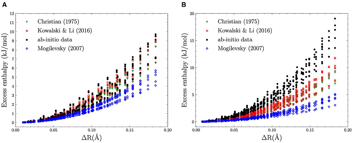
Figure 1. The excess enthalpy of mixing for (A) monazite-type and (B) xenotime-type solid solution computed ab initio and from models of [36], [34], and [26].

The situation is diametrically different in the case of xenotime-type solid solutions (Figure 1B). Here, the models of [36] and [34] give predictions that are inconsistent with the ab initio data by a factor of ~ 2. This points toward the possibility of another unaccounted term in the Margules parameter that could be quite relevant in the case of xenotime-type solid solutions but of minor importance for monazite-type solid solution.

A combination of ab initio and calorimetric studies [37] has shown that the ab initio data themselves are not enough to constrain the values of the Margules parameter W, and that understanding of the dependence of W on the selected physical parameters is crucial for precise modeling of the stability of solid solutions. As such, the study of the excess of enthalpy for this type of solid solutions lends itself perfectly to test the explainable machine learning methodology we have devised.

2 Methodology and learning algorithms

In predicting materials' properties, one needs a set of curated training data organized in input variables x and target properties y. The set of input variables has to represented in terms of a number of independent descriptors that are invariant under known mathematical and physical symmetries and usually requires a considerable amount of domain expertise. In this study, the input variables are represented by properties of the elements constituting a solid solution (e.g., electron orbitals, nuclear charge, etc.) and the target property by the solution excess enthalpy of formation.

2.1 Elemental properties and descriptors

As mentioned in [10], a limited number of selected atomistic properties carry most of the weight in determining the value of the enthalpy of formation of metal and non-metal compounds such as Pauli electronegativity, Volume, Ionic radius. In similar studies [11, 13], properties associated with the electron orbitals and macroscopic properties, such as the total ground energy, are shown to contribute the most in determining the value of the enthalpy of formation. These evidence-based observations seem to suggest a universal trend that is common to most of compounds in chemical space.

Based on the physics of the formation process of the Lanthanides Orthophosphates solid solution, it is a very plausible assumption that also in this case, a limited number of microscopic and macroscopic properties contribute to H^E. Moreover, all solid solutions that are part of our dataset have in common the same phosphate group (PO₄). Consequently, properties of the atomic elements of such group are not taken into consideration. Based on the consideration made in the previous section on the first leading term contributing to the enthalpy and on the experience of domain practitioners, we have chosen nine basic elemental properties (elementals) ϵ_k, as shown in Table 1, that are available for each and every lanthanide element. Their values for each Lanthanide are extracted from the online database http://www.knowledgedoor.com/.

Table 1

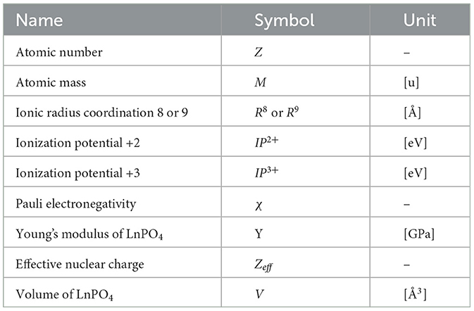
Table 1. List of elemental properties and their physical units.

These elementals can be arranged in an abstract vector $ϵ={({ϵ}_1,{ϵ}_2,\dots )}^T={(Z,M,R^{8,9},I{P}^{2+},I{P}^{3+},\dots )}^T$. For each lanthanide L_i ∈ (La, Ce, Pr… ), there is one such vector. We build descriptors out of elementals. Since we are investigating solid solutions made of two lanthanides, our descriptors x_k[ϵ_k(L_i), ϵ_k(L_j), m_i, m_j] are functions of elementals from two different lanthanides together with their mixing ratio m_i. The inclusion of m_is is necessary to distinguish between different solution ratios. However, the descriptor is defined, and it should be invariant to simultaneous permutation of lanthanide and mixture ratios. Noting that m_i + m_j = 1, we can actually use only one mixing ratio m = m_i so that m_j = 1 − m.

Invariance under permutation can be expressed as follows:

$x_k\left[{ϵ}_k(L_i),{ϵ}_k(L_j),m\right]=x_k\left[{ϵ}_k(L_j),{ϵ}_k(L_i),1-m\right]$

is important that a descriptor x changes significantly with the mixing ratio. Additionally, one should include descriptors capturing certain processes where the enthalpy is strongly dependent on which lanthanide has the largest abundance. Last but not least, descriptors have to be homogeneous functions of elementals and cannot mix elementals with different physical units (unless conversion constants are involved). For the reasons above, we selected three types of descriptors x⁽¹⁾, x⁽²⁾ and x⁽³⁾, as shown in Table 2, for every elemental ϵ_k and every lanthanide pair (L_i, L_j).

Table 2

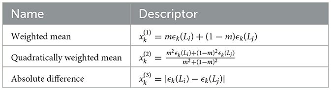
Table 2. Descriptor types depending on lanthanide pairs (L_i, L_j), elemental ϵ_k, and mixing ratio m.

Notice that the quadratically weighted mean is not quadratic in the actual values of the elementals ϵ_k but quadratic in the mixture ratio m. The descriptor x⁽²⁾ will lean heavily to the value of the elementals of the more abundant lanthanide. For each combination of lanthanide pairs, the nine elementals ϵ_k are organized in a descriptor vector x made of 27 descriptors in total.

$\begin{array}{l}x(L_i,L_j,m)=\left[\begin{array}{c}{x}_1^{(1)}\left[{ϵ}_1(L_i),{ϵ}_1(L_j),m\right]\\ x_1^{(2)}\left[{ϵ}_1(L_i),{ϵ}_1(L_j),m\right]\\ x_1^{(3)}\left[{ϵ}_1(L_i),{ϵ}_1(L_j),m\right]\\ x_2^{(1)}\left[{ϵ}_2(L_i),{ϵ}_2(L_j),m\right]\\ ⋮\end{array}\right]\end{array}$

Each vector $x\in \mathcal{X}$ of size d = 27 makes up the input variables for the learning algorithm. The target value y is the excess enthalpy of formation H^E. For each choice of lanthanide pairs (L_i, L_j) and choice of mixing ratio m, we have a data point (x, y). All data points together constitute a set holding N data points. We will observe at the end of this section how this set of points is generated.

2.2 Learning algorithms

Since the data points in our set have both input values and target value, we use a common type of supervised learning algorithm: kernel ridge regression (KRR) [12]. Kernel ridge regression is a non-linear regression algorithm with a regularization term (from which the name “ridge”) that is comparable to the well-known Support Vector Machine algorithm.

The simple linear regression algorithm aims at finding the unknown coefficients β of the function $f(z)=\langle \beta ,z\rangle ,z\in \mathcal{X}$ minimizing the error E[f(z)−y] (also known as loss function) over the entire set of data. To alleviate over fitting of the data, a regularization term is usually added. In the ridge regression, the regularization amount to adding a penalty term to the minimization problem. Choosing the squared error as loss function leads to the following minimization problem

$\begin{array}{ll}arg{\displaystyle \underset{\beta \in {ℝ}^d}{min}}{\displaystyle \sum _i}{(\langle \beta ,x_i\rangle -y_i)}^2+\lambda ||\beta {||}_2^2& (2)\end{array}$

By introducing a function z → ϕ(z) which maps the input space $\mathcal{X}$ to a feature space $\mathcal{H}$, the use of kernels generalizes the linear to non-linear regression [see [38] for a didactic introduction]. In this context, a kernel is an inner product in feature space k(x_i, x_j) = 〈ϕ(x_i), ϕ(x_j)〉. The advantage of using kernels is that the function $f(z)=\sum _i{\alpha }_{i}k(x_i,z)$ is not expressed anymore as a sum over dimension d of the input space, instead as a sum over the number of data N making up the training set. With this set up, the minimization problem of Equation 2 becomes

$\begin{array}{l}arg{\displaystyle \underset{\alpha \in {ℝ}^N}{min}}{\displaystyle \sum _i^N}{(f(x_i)-y_i)}^2+\lambda ||f{||}_{\mathcal{H}}^2,\end{array}$

with $||f{||}_{\mathcal{H}}^2=\sum _j\sum _i{\alpha }_j{\alpha }_{i}k(x_i,x_j)$. In practice, the kernel function is expressed as a matrix of inner products between points of the training data set in feature space k(x_i, x_j) = K_ij. Eventually, the solution of the minimization problem can be expressed by the linear equation

$\begin{array}{ll}\alpha ={(K+\lambda 1_N)}^{-1}y,& (3)\end{array}$

with α ∈ ℝ^N being the vector that contains the information learned.

Almost all Machine Learning methods do not work directly out of the box but have a number of parameters that have to be fixed. In the case of the KRR, the level of regularization through the parameter λ is tuned for the dataset at hand and the selected kernel. Additionally, almost every kernel has some extra parameters that must also be tuned. The entire set of these adjustable parameters is called hyperparameters.

Given a kernel, its computation can still be performed in input space, despite its value describes the inner product in feature space. In this study, we employed three different kernels with the same set of data: the polynomial, the Gaussian, and the Laplacian kernels, which are, respectively, based on the inner product, the ℓ₂-norm, and the ℓ₁-norm

$\begin{array}{ll}k(x,z)={(\langle x,z\rangle +c)}^p& (4)\end{array}$

$\begin{array}{ll}k(x,z)=exp\left(-\frac{{||x-z{||}_2}^2}{2{\sigma }^2}\right)& (5)\end{array}$

$\begin{array}{ll}k(x,z)=exp\left(-\frac{||x-z{||}_1}{\sigma }\right).& (6)\end{array}$

The actual computation of α amounts to solve a positive-definite numerical linear system Aα = y. Once α is computed, it is used to compute predictions for any new data point with $ŷ=\sum _i{\alpha }_{i}k(x_i,\widehat{x})$. For validation purpose, the results of such prediction are typically presented in a scatter plot where the predicted and computed target values are represented on x and y, respectively (see plots of Figure 2, for instance).

Figure 2

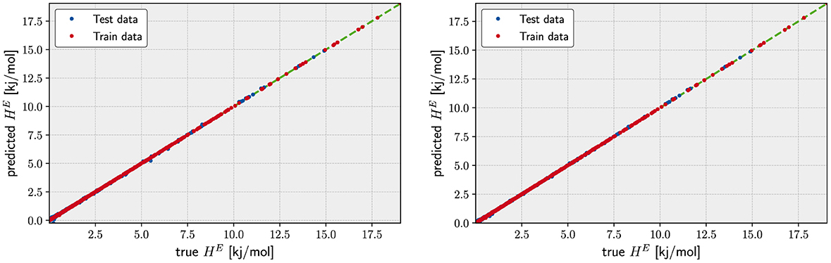
Figure 2. Regression for the Gaussian Kernel (left) and the degree 3 polynomial Kernel (right). The scatter plot corresponds to a trained model whose hyperparameters have been already fitted. Gaussian best fit: λ = 10^−13.46, γ = 10^−5.90 with an MAE of 1.07 × 10⁻² kJ/mol. Degree 3 polynomial the best fit: λ = 10^4.73, γ = 10^5.79, c = 10^0.37 with an MAE of 9.00 × 10⁻³ kJ/mol.

The Laplacian (Equation 6) and Gaussian (Equation 5) kernels are by far the most used in KRR because they provide the most effective map since they use a virtually limitless number of functions as the prior of our statistical model. On the other hand, our aim is to employ a set of kernels that use only a finite number of functions and could be, in theory, inverted. Once (approximately) inverted, such kernels, which, in this study, are represented by the polynomial kernels of increasing degree, could return a functional expression for the coefficients α in terms of the descriptors. Being able to statistically infer such functional expression would allow us to go beyond the prediction of target values for new solid solutions and understand which descriptors are more relevant and contribute the most to determine the target values. Moreover, in applying KKR, we focus on polynomial kernels and use the accuracy of results coming from Gaussian and Laplacian to monitor how closely the accuracy of the former come to the latter. In this sense, the polynomial kernels that will be closest in error to the Gaussian or Laplacian kernels will provide a hint on the order of polynomial functions that should be included in our previous study.

With this information, we can manually construct thousands of candidate functions of the original elementals $x_i^{(t)}$ that could faithfully represent the underlying surrogate space. In our application, we refer to these candidate functions as v = [v₁; v₂; ⋯ ;v_M], where M can range from $\mathcal{O}(10^3)$ to $\mathcal{O}(10^4)$. Each v_k is a function of one of more $x_i^{(t)}$ up to degree p. For example, a degree 3 function could be $x_2^{(7)}{(x_3^{(3)})}^2$. We then apply a sparsification technique, which amounts to find the most relevant among the v_k by forcing as many coefficients of the statistical model to be zeros. In Section 3.1, justified by the KRR results, we show how each distinct v_k is constructed from the all possible polynomial functions of the original descriptors up to degree p.

The objective of sparsification is finding the most relevant term(s) among v_k which contributes the most to the target values. Moreover, the number of the relevant terms should be also controllable. A straightforward sparsification technique that one can employ is the LASSO [15] approach where the ℓ₁ is substituted with an ℓ₀ regularization. This combination is able to sparsify the coefficients of LASSO regression into a small determined number. The minimization problem to be solved is given as follows:

$\begin{array}{ll}arg{\displaystyle \underset{\gamma \in {ℝ}^M}{min}}{\displaystyle \sum _i^N}{(\langle \gamma ,v_i\rangle -y_i)}^2+\widehat{\lambda }||\gamma {||}_0.& (7)\end{array}$

In this formula, the ℓ₀-norm of a coefficient vector γ is defined as follows:

$\begin{array}{l}||\gamma {||}_0=\#\left\{j:{\gamma }_j\ne 0\right\},j=1,\dots ,M\end{array}$

indicating the number of non-zero elements of the γ vector. A vector γ ∈ ℝ^M is called κ-sparse if ||γ||₀ ≤ κ.

While the minimization with the ℓ₀ regularization is the exact problem we want to solve, it has a significant drawback: this minimization problem is not convex. This leads to an “NP-hard problem” ¹ which is infeasible when M is large. Therefore, ℓ₀ cannot be directly applied to sparsify the candidate functions in v. To compromise between the convexity and sparsity of the coefficient vector, we first utilize a Manhattan ℓ₁-norm regularization λ||γ||₁ (which is the standard definition of LASSO) to carry out an initial feature selection, out of which we can achieve the sparsification of v [14].

$\begin{array}{ll}arg{\displaystyle \underset{\gamma \in {ℝ}^M}{min}}{\displaystyle \sum _i^N}{(\langle \gamma ,v_i\rangle -y_i)}^2+\widehat{\lambda }||\gamma {||}_1.& (8)\end{array}$

This latter optimization problem is convex, which promote also sparsity. In Equation (8), $\widehat{\lambda }>0$ is the penalty parameter which is able to control the sparsity of the coefficient vector v: the larger $\widehat{\lambda }$ is, the smaller the ℓ₁-norm ||γ||₁ would be, hence higher sparsity is achieved and more candidate functions are eliminated.

In our application, we start from a very small $\widehat{\lambda }$, then increase it with a fixed step. With the increase in $\widehat{\lambda }$, we observed that a large number of constructed functions in v gets quickly eliminated to rapidly flatten the curve which stagnates even for much larger λ values; in other words, the minimization process with the ℓ₁-norm reduces the vector γ to be at most κ-sparse, κ being ~20 in our application. In practice, we compressed a very large feature space spanned by v into a tiny one spanned by v′, in which v′ is a subset of v whose number of elements is smaller than κ. Due to the low dimension of feature space selected by LASSO, the Equation (7) can be solved for v′ in place of v rather effectively with a brute force approach. More details of numerical results are shown in Section 3. In the rest of the study, we refer to the use of LASSO together with the further sparsification using an ℓ₀ regularization as LASSO+ℓ₀.

This method, combining LASSO with a sparsification of the coefficient vector, has been developed in the context of compressed sensing [14], where one is interested in reproducing the gathered data with as few as possible degrees of freedom. Unlike the article in the study mentioned in [14], our approach starts with a Kernel Ridge Regression and maps the descriptors x_i to a much larger but finite dimensional input space, where the new features v_k are made out of a finite number of selected functions of the original descriptors x_i. We additionally integrate domain-knowledge by modifying the initial selection of descriptors and features to ensure scientific consistency with the existing knowledge from the physics of solid solutions. The necessity of tuning of the descriptors and the features is also confirmed by the inefficiency of the LASSO method when the original descriptors x_i are used.

In the next section, we observed that KRR polynomial kernel with degree p = 3 returns one of the lowest statistical error. We capitalize on such a result and make the plausible hypothesis that a polynomial map of degree at most 3 for LASSO should identify the most promising functions of the descriptors $x_k^{(t)}$. We then show that the results of feature selection by LASSO suggest the selection of a modified set of descriptors that guarantees scientific consistency. Finally, through the ℓ_o regularization, we determine the desired functions which map the elemental descriptors to the excess of enthalpy for both monazite and xenotime.

2.3 Dataset generation

The dataset used by the selected learning methods was computed with the Quantum-ESPRESSO code using the approach of [28, 34]. The solid solutions were modeled with special quasi-random structures constructed using procedure of the study mentioned in [39]. All the structures were modeled with supercells containing 192 atoms (32 formula units). We applied the PBEsol exchange-correlation functional [40], and the f electrons were included into the pseudopotential core. It has been shown that this setup results in a very good predictions of structures and thermodynamic parameters of lanthanide phosphates, including formation enthalpies [30, 32, 41, 42]. The excess enthalpies of mixing and Margules interaction parameters were derived from differences in the total energies of the mixed cation structure and weighted (according to the solid solution composition) sum of the end members.

The dataset consists of excess enthalpies of formation among all 15 lanthanides, which leads to 105 possible combinations ($\sum _{i=1}^{14}i=105$). Those 105 combinations were then modeled for five different mixture ratios m = 0.25, 0.375, 0.50, 0.625, and 0.75, giving 525 data points. Two distinct datasets were generated for the two lanthanide orthophosphate phases, monazite and xenotime, which correspond to the two possible coordination numbers, R⁸ and R⁹, of the lanthanides (see Table 1). In the following, we will test our models on three distinct configurations of these data: monazite only (525 data points), xenotime only (525 data points), and fused (1, 050 data points). Not all these points are used to train the learning model. A subset is reserved for testing and validation purposes.

All the data and the scripts used to generate the results presented in this study are publicly available at https://github.com/SimLabQuantumMaterials/MLESS.

3 Regression, sparsification, and interpretable formulas

The first step before determining the coefficients α of our KRR models is to determine the optimal value of the corresponding hyperparameters. To this aim, the entire given dataset is typically split in to two parts. The training dataset $(x_i,y_i)\in \mathcal{T}$ is used to compute the actual coefficients α of the regression that appear in Equation (3). The testing or prediction dataset $({x^{\prime }}_i,y_i^{\prime })\in \mathcal{P}$ is separate and is used to evaluate the quality of a given set of hyperparameter values for predicting unseen data ŷ = α^𝖳K′, where $K_{ij}^{\prime }=k(x_i,{x^{\prime }}_j)$. The optimal set of parameters is selected when the predictions (i.e., ŷ_i) are in the best possible agreement with the known values from the testing dataset (i.e., $y_i^{\prime }$). Different error functions are commonly used to quantifying the quality of a prediction. The most common are the Mean Squared Error (MSE), Mean Absolute Error (MAE), and Maximum Error (ME). In this study, we use exclusively the MAE

$\text{MAE}=\frac{1}{N}{\displaystyle \sum _i}|{ŷ}_i({x^{\prime }}_i)-y_i^{\prime }|,$

because it is the one giving the most sensible measurement of error throughout the entire set of solid solutions.

Because possible hyperparameter values may span over multiple dozens of orders of magnitude, brute force methods that quickly scan the entire space in a grid-like pattern are preferred to conventional minimization methods. Once an approximate local minimum is found, local optimizations are used to refine the values of the hyperparameters. In the following, we do not report the hyperparameter search results which is a standard procedure in the use of ML algorithms. In all the scatter plots and tables, it is implicitly intended that all hyperparameters have been opportunely optimized following the procedure just described.

3.1 Predicting excess of enthalpies with KRR

In the search for optimal hyperparameters, we have split the total subset of data in to two parts between $\mathcal{T}$ and $\mathcal{P}$. The ratio of the data size between $\mathcal{T}$ and $\mathcal{P}$ is 4:1. Once the hyperparamete search is completed, we fitted the data of the training set $\mathcal{T}$ using all three distinct kernels for the KRR model. It has to be noted that instead of the standard polynomial formulation of Equation (4) K(x, y) = (x^𝖳y+c)d, we have used a slightly modified kernel k(x, y) = (γx^𝖳y+c)d that produces slightly better results. Additionally, we unified the notation and used the symbol γ for both multiplicative factors changed to k(x, y) = exp(−γ·||…||) (the $\frac{1}{2{\sigma }^2}$ and $\frac{1}{\sigma }$ for the Gaussian and Laplacian kernels, respectively).

In Table 3, we report the results obtained for all kernels with MAE for both sets $\mathcal{T}$ and $\mathcal{P}$ on the fused data set configuration (similar results are obtained for the other two configurations). Despite its remarkable low errors on the $\mathcal{T}$ set, the Laplacian kernel does not return a satisfactory result on the set of prediction data $\mathcal{P}$. In fact, no choice of hyperparameters returns a reliable regression for unseen data: the search space minimization return a value for λ numerically indistinguishable from zero. This is a typical sign that KRR with this kernel is overfitting the data and returning an in-sample error much smaller of the out-of-sample error. For this reason, we discarded the learning model using the Laplacian kernel.

Table 3

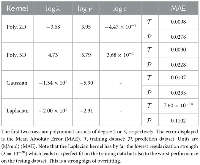
Table 3. Kernel Ridge Regression results on the Excess Formation Enthalpy dataset for different Kernel types.

The low order polynomial and the Gauss kernels return a much nicer picture in terms of the errors. Already the degree 2 polynomial kernel is able to fit the data quite well. Its MAE differs only ≈ 1 × 10⁻³ kJ/mol from the error of the degree 3 kernel and the Gaussian Kernel. Judging from the fact that the degree 3 polynomial kernel returns an MAE as low as ≈ 2 × 10⁻² kJ/mol for the $\mathcal{P}$ set which indicates that the underlying function for the excess of Enthalpy could be represented by functions of the descriptors having up to cubic terms. Since the actual values for the excess enthalpy of the formation for the lanthanide orthophosphates span a range going from of 0.5 to 1.00 × 10¹ kJ/mol, the relative errors of our model represent the same level of uncertainty returned by the DFT simulations. In other words, the prediction provided by the KRR model with either a degree 3 polynomial or the Gauss kernel are indistinguishable from the finite accuracy of the in silico simulation used to generate the data used in both sets $\mathcal{T}$ and $\mathcal{P}$ (see Figure 2).

What distinguishes the Gaussian and the degree 3 polynomial kernels are the value of the hyperparameters: the degree 3 kernel requires a quite large value of λ and γ respect to the Gaussian. This is not necessarily a negative result but it points out that our choice of descriptors may not be ideal when the kernel represents a finite set of prior functions such as in the case of the degree 3 polynomial. When the set of prior functions becomes virtually infinite (the Gaussian kernel can be observed as an infinite series of polynomials), the descriptor choice becomes unimportant. We will observe in the following subsection how the choice of descriptors becomes significant when one would like to sparsify the vector of coefficients α starting from a finite set of prior functions of the descriptors.

To ensure that our KRR models provide a good fit for all data independently on how they are split between $\mathcal{T}$ and $\mathcal{P}$, we have used cross validation. In practice, we run the KRR models, fitting several different choices of training and testing datasets always keeping the same choices of values for the hyperparameters that were previously selected. If the results with the original dataset were truly a product of chance, a fit with an entirely new combination of data points should show a different performance. Table 4 shows the results for repeating the KRR with polynomial kernel of degree 3 for five different subsets, some of which even showed slightly better performance than the original regression. The MAE over the five different sets ranges between 0.052 and 0.082 kJ/mol, confirming the quality of the original regression.

Table 4

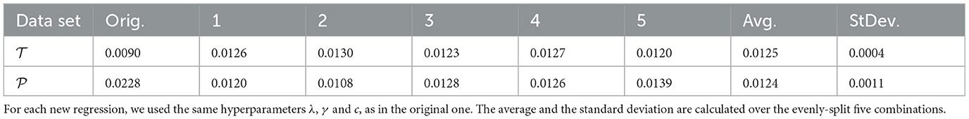
Table 4. MAE (kJ/mol) of the excess of enthalpy for the cross-validation of polynomial kernel of degree 3 with five different combinations of data points evenly split between $\mathcal{T}$ and $\mathcal{P}$.

3.2 LASSO + ℓ₀

In the previous section, we have concluded that KRR with Gaussian and degree 3 polynomial kernel performs very similarly with a slight advantage for the latter kernel. In this section, we want to pursue the road of finding a surrogate model that is explainable: we aim at formulation of the excess enthalpy of mixing that can provide the domain scientist with an understandable function of a small number of descriptors. We are driven to recover this result by the observation that already polynomial functions of degree 3 provide enough prior to get an accurate KRR model. We achieve this result through a so-called sparsification process.

3.2.1 Sparsification with descriptors in KRR

A large number of candidate functions have been built from the polynomial kernel of degree 3 based on the 27 elemental descriptors introduced in Section 2.1. Denoting the group of 27 elemental descriptors as ${\mathcal{D}}_1$, a group of candidate functions with polynomial of degree 2, denoted as ${\mathcal{D}}_2$, can be defined as a commutative element-wise vector product d_id_j, with $d_i,d_j\in {\mathcal{D}}_1$. The number of descriptors in ${\mathcal{D}}_2$ is 378. The group of candidate functions with polynomial of degree 3, denoted as ${\mathcal{D}}_3$, can be defined in a similar way, as a commutative element-wise product of three vectors d_id_jd_k with d_i, d_j, $d_k\in {\mathcal{D}}_1$. The number of descriptors in ${\mathcal{D}}_3$ is 3.30 × 103. Therefore, all the candidate functions are a union of ${\mathcal{D}}_1$, ${\mathcal{D}}_2$, and ${\mathcal{D}}_3$, which is denoted as $\mathcal{D}$. $\mathcal{D}$ is a dense matrix of size 1, 050 × 3, 708 for the fused data set and of size 525 × 3, 708 for both monazite and xenotime data set configurations.

As described in Section 2.2, a feature selection step has been performed on $\mathcal{D}$ through the LASSO method. Increasing the penalty parameter λ, the size of feature space is reduced as more candidate functions are removed. In the numerical experiments, λ is increased from 1 × 10⁻³ to 9.60 × 10⁻² in incremental steps of 5 × 10⁻³. We performed the same feature selection step not only for the fused data but also separately for monazite and xenotime data configurations. The results are shown in Figure 3, which shows the variation of the MAE and the size of the reduced feature space.

Figure 3

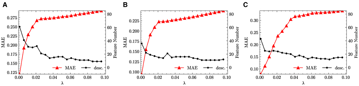
Figure 3. LASSO results with descriptors used in KRR. (A) Fused. (B) Monazite. (C) Xenotime.

From Figure 3, we infer that with the increase of λ, the feature space size can be quickly reduced to <30. This is good news, since sparsifying a feature space of size ~ 3.00 × 101 through LASSO+ℓ₀ into a determined size smaller than 5 is still feasible². At the same time, we observed that all the errors increase with the increase of λ. This behavior is to be expected and is the direct consequence of the reduction of the feature space size. Unfortunately, the errors increase too quickly and show an exponential growth that plateaus already for small values of λ. For example, for fused data, the MAE increases from ~ 3 × 10⁻² to more than 2.50 × 10⁻¹ when λ is only increased from 1 × 10⁻³ to 2.10 × 10⁻². When increasing λ from 0.021 to 0.096, the feature space size continues to be reduced however, the changes of error flatten. Similar trends can also be observed separately for the monazite and xenotime data. This result signals that the generated feature space does not capture well the functional dependence of the excess enthalpy on the descriptors. In other words, we cannot find a simple functional dependence of H^E and need many hundreds of functions to faithfully predict the enthalpy.

To confirm our concerns, we perform a LASSO+ℓ₀ step on the reduced feature space separately for the fused, monazite, and xenotime dataset configurations. At most, three leading terms have been selected, which are shown in Table 5, along with their corresponding MAEs. As expected, the errors of candidate functions selected by LASSO+ℓ₀ are more than one of order of magnitude larger than the ones derived by KRR. What is more remarkable is the fact that the errors do not seem to decrease much as we consider more terms. In fact, for the fused data configuration, the MAE actually increases going from 2 to 3 leading terms. The errors for the other data configuration seem a bit better but are still far from what we would like to observe. From these tables and the plots shown in Figure 3, we conclude that the choice of prior candidate functions cannot be effectively exploited by the sparsification process.

Table 5

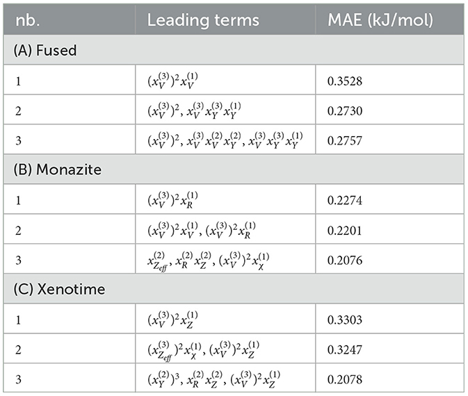
Table 5. LASSO+ℓ₀ results for fused, monazite, and xenotime with descriptors used in KRR.

3.2.2 Sparsification with descriptors built with prior knowledge

To overcome the shortcomings of the sparsification process seemingly caused by the choice of descriptors, we simplify the form of the descriptors and exploit the existing knowledge from the application domain. Based on the insight provided by the simple model with the Margules interaction parameter W and the expression in Equation (1), we make three additional assumptions: (i) the polynomial degree of m and 1 − m may not be in accordance with each other and the polynomial degree of the elemental property ϵ_k, (ii) negative power of the descriptors may appear in the Margules parameter and, (iii) the volume V, ionic radius R, and mixing ratio m play a special role than the other elemental properties and may contribute with monomials of degree higher than 3.

The direct consequence of (i) is that m and 1 − m have been decoupled from the elemental descriptors and included as descriptors on their own. This may seem a strange choice since they do not depend on the lanthanides but are the same for all. On the other hand, decoupling the mixing ratio allows more freedom in the way it appears in the degree 3 polynomial functions that are part of $\mathcal{D}$. The indirect consequence is that we do not have anymore three types of descriptors for each elemental property ϵ_k but only two: we drop the weighted quadratic mean, convert the weighted mean to a simple arithmetic mean, $\overline{{ϵ}_k}$ and keep the absolute difference Δϵ_k (see Table 6).

Table 6

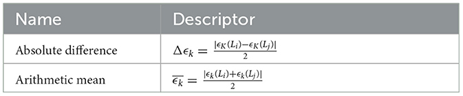
Table 6. Two basic descriptors of elemental property ϵ_k.

The second hypothesis implies that the inverse of each elemental property Δϵ_k and $\overline{{ϵ}_k}$ is also included explicitly in the descriptor. Additionally, due to the third hypothesis, we include as descriptors monomials of degree higher than one for m, V, and R. In particular, for m, and 1 − m we include up to quadratic terms (and their inverse), and for V and R, we include up to cubic terms (and their inverse).

All these descriptors build up a basic feature space ${\mathcal{D}}_1$ of size 58. Analogously as done for the original descriptors, the groups ${\mathcal{D}}_2$ and ${\mathcal{D}}_3$ are built as the element-wise product of two or three features out of ${\mathcal{D}}_1$, respectively. Feature space ${\mathcal{D}}_2$ is of size 1647 after removing 6 features with standard deviation being 0, such as the element-wise product of $\frac{1}{m}$ and m. The size of feature space ${\mathcal{D}}_3$ is 30, 856. The sum of all candidate functions is collected into $\mathcal{D}={\mathcal{D}}_1\cup {\mathcal{D}}_2\cup {\mathcal{D}}_3$. The size of data $\mathcal{D}$ is 1, 050 × 3, 2561 and 525 × 32, 561 for fused and monazite/xenotime data configurations. These choices imply that terms can have orders higher than degree 3 for m, m − 1, V, and R. For example in Table 7(C), one can have the term $\frac{{(\Delta V)}^2}{{(\overline{V})}^3\overline{V}}$ which is in the form d_id_jd_k, with $d_i={(\Delta V)}^2$, $d_j={(\overline{V})}^{-3}$, and $d_k={(\overline{V})}^{-1}$.

Table 7

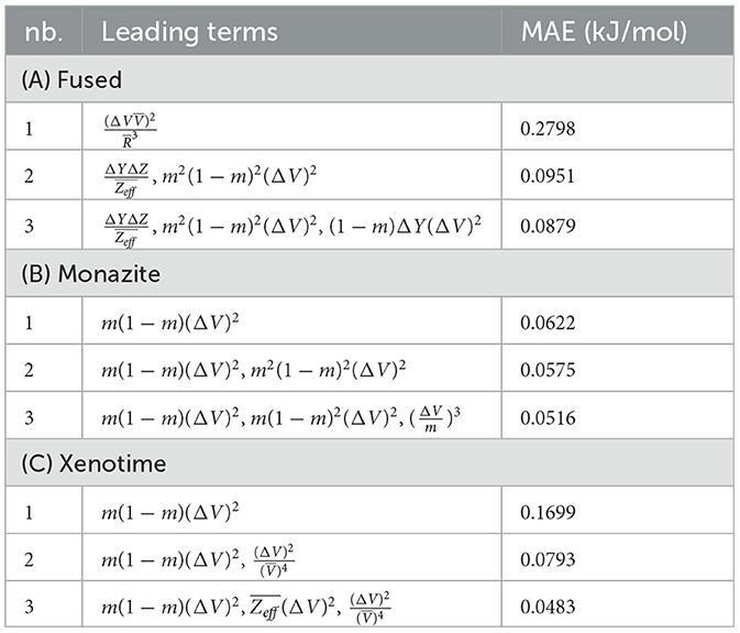
Table 7. LASSO+ℓ₀ results for fused, monazite, and xenotime with descriptors defined only by arithmetic means and absolute difference.

We run the same LASSO as in Section 3.2.1, the results of which are shown in Figure 4. Compared with the Figure 3, the results we obtained are quite more promising. For fused data in Figure 4, the size of reduced feature space drops down quickly below 40 which is already at very small value of λ. Afterward, with the increase of λ, the decrease in the size of reduced feature space slows down, which implies that the reduced feature space contains always important features for the target problem. Meanwhile, with the increase of λ, the errors increase moderately and linearly, which is a second sign that the feature space is reduced into a good choice of representative functions.

Figure 4

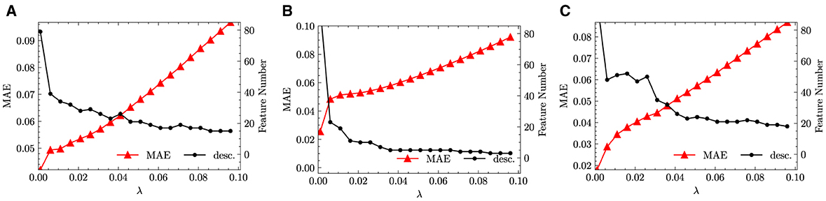
Figure 4. LASSO results with descriptors defined only by arithmetic means and absolute difference. (A) Fused. (B) Monazite. (C) Xenotime.

After applying LASSO+ℓ₀ on the vector of descriptors spanning the reduced space, the first three leading terms and their corresponding errors for fused, monazite and xenotime data configurations are shown in Table 7. It is important to notice that while the errors may still be quite high for keeping only the leading term, they decrease rapidly when we include higher terms. Moreover, the first leading term for the monazite, and xenotime data configurations resemble closely the expression of Equation (1). We will analyze in more details the results and interpret their physical meaning up to five leading terms in the next section.

4 Numerical results

As shown in Section 1.1, the discrepancies between existing models and the data make the computation of the excess of enthalpy for solid solutions of both monazite and xenotime, a clear cut example to demonstrate the validity of our statistical approach in retrieving an explainable expression for H^E. We will (1) show which descriptor provides the most reliable leading term for the mixing enthalpy between ionic radii of the mixing cations and the volumes of the pure phases, (2) identify the first sub-leading term, which enhances the accuracy of the H^E prediction of xenotime-type solid solutions.

To address the points (1) and (2), we apply the sparsification integrated with previous knowledge to a variety of scenarios: (i) using all modified descriptors illustrated in Section 3.2.2, (ii) using all modified descriptors excluding the one based on ionic radii elementals R⁸ and R⁹, (iii) using all modified descriptors excluding the one based on the volume elemental V, and (iv) using only descriptors based on the volume V, mixing ratio m and Young modulus Y elementals. In addition, we used three different sets of data—monazite, xenotime, fused—for each of the four cases (i)–(iv). In total, we produced 12 separate sparsification scenarios, each specifying functions up to five leading terms and the relative errors. In the analysis that follows, we remind the reader that all the numerical coefficients are not dimensionless and may carry different SI units. Consequently, we cannot compare coefficients across terms featuring distinct elemental descriptors.

The (1) statement is inferred from the direct inspection of cases (ii) and (iii) over the fused data set (see Tables 8, 9). Comparing the two tables, one can observe that several functions where ΔV appears in Table 8 correspond to similar functions of ΔR in Table 9. On the other hand, the MAE is comparatively smaller in Table 8 than Table 9 for any count of descriptor number. This is suggestive of the fact that either the ionic radius or the volume should be included in the list of elemental properties. TP understand which among these two elemental properties should be eliminated, we look next to the cases (ii) and (iii) applied separately to monazite (Tables 10, 11) and xenotime (Tables 12, 13) data sets. Comparing the MAE, one notices that descriptors without the volume V return always larger errors than descriptors without the ionic radius R, for both monazite and xenotime data sets. This is a strong indication that V should be preferred over R as the elemental property of choice. This concludes statement (1) and excludes from further analysis cases (i) and (iii) which include R.

Table 8

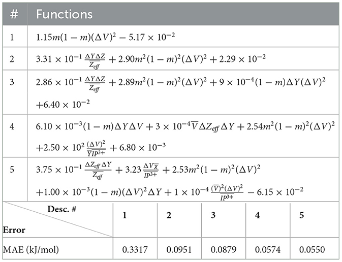
Table 8. Fused: all elemental descriptors except Ionic radius coordination.

Table 9

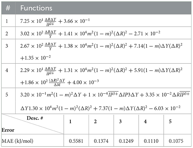
Table 9. Fused: all elemental descriptors except volume.

Table 10

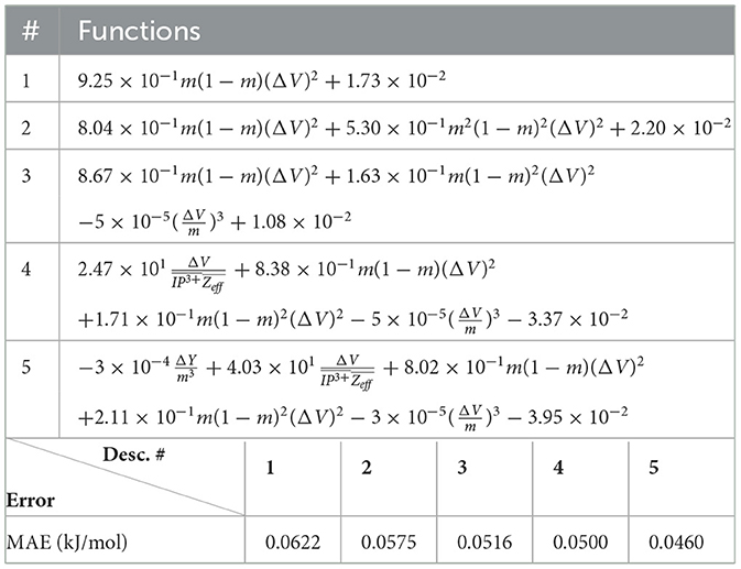
Table 10. Monazite: all elemental descriptors except Ionic radius coordination.

Table 11

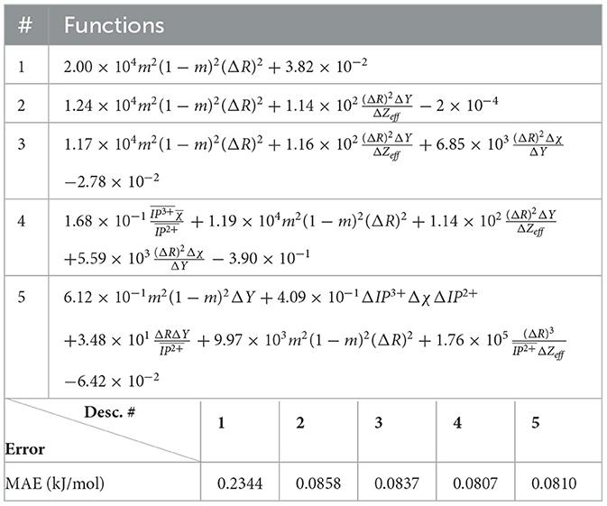
Table 11. Monazite: all elemental descriptors except volume.

Table 12

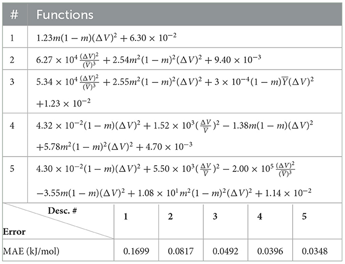
Table 12. Xenotime: all elemental descriptors except Ionic radius coordination.

Table 13

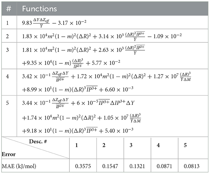
Table 13. Xenotime: all elemental descriptors except volume.

Next, we look at cases (ii) and (iv) applied to all three sets of data (Tables 10, 14 for monazite, Tables 12, 15 for xenotime, and Tables 8, 16 for fused). The first observation is that no matter what dataset or case one looks at, all the one-term functions are of the form m(1−m)(ΔV)². Unequivocally, this is the first leading term describing the excess enthalpy, H^E. We also notice that sub-leading terms for monazite and xenotime datasets are dominated by the volume elemental but this dominance manifests itself differently for each distinct dataset and with errors that vary from case to case. For xenotime, the prediction of H^E with only one term returns an MAE which is twice the one for monazite indicating that additional terms are needed to get better accuracy. In both data sets, the leading term is m(1−m)ΔV², but the numerical coefficient for xenotime is substantially larger than the one obtained for monazite (1.23 vs. 0.94). Although this difference could be possibly explained with on average larger Young's moduli of xenotime phases than monazite [see Equation (1)], this observation also indicates that additional terms are essential to obtain an equation that consistently described both structures. When we look at the results for xenotime alone (Tables 12, 15), there is some discordance between sub-leading terms usually involving some power of the difference and the average of the volume and/or the Young's modulus. We conclude that only simultaneous fit to monazite and xenotime datasets could shed light on the functional form of the sub-leading terms.

Table 14

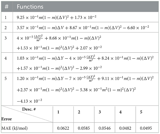
Table 14. Monazite: only Volume and Young modulus.

Table 15

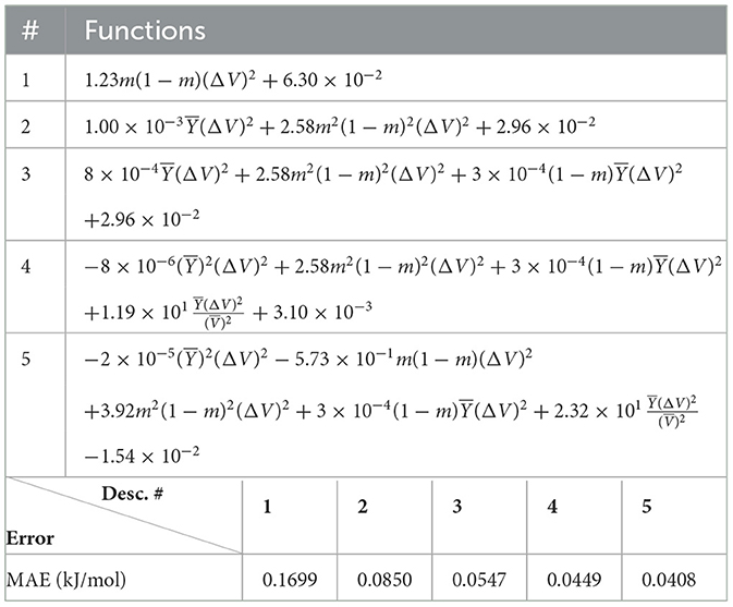
Table 15. Xenotime: only Volume and Young modulus.

Table 16

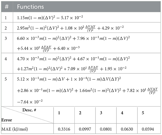
Table 16. Fused: only Volume and Young modulus.

Looking at the fused data (Tables 8, 16), it becomes clear that both the volume and the Young modulus Y play a central role in many of the sub-leading terms: Using descriptors of only V and Y consistently returns smaller MAEs. Incidentally, Young's moduli and volumes/ionic radii are the elemental properties used in models [26] and [34]. To provide some clearer evidence of this statement, we focus on the leading and sub-leading terms shown in Table 16, where all elementals apart from m, V, and Y are discarded. The second leading term contains product of ΔV and ΔY. Combining the two terms m(1 − m)ΔV² and $\Delta Y\Delta V/{\bar{V}}^2$, one can satisfactorily express H^E for both sets of data.

This indicates that in addition to difference in volume, the difference in Young's modulus plays a significant role in determining the excess of enthalpy of mixing. To better understand the role of this second term, we plot in Figure 5A the variation of Young's modulus as a function of ΔV for the two phases. For the considered range of elastic moduli and volumes, there is a clear linear relationship between the two. However, the linear relationship is much steeper for xenotime than monazite, with the slope about three times higher in the former case. This makes the $\Delta Y\Delta V/{\bar{V}}^2$ term much larger (by a factor ~3) for the xenotime, putting it on equal footing with the leading term m(1 − m)ΔV². This explains why the absence of this term, in the description of xenotime-type solid solutions, causes a discrepancy of a factor ~2 between the ab initio data and the previously discussed theoretical models (see Figure 1).

Figure 5

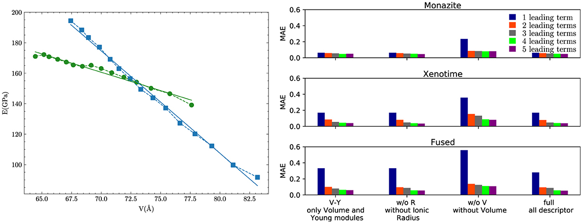
Figure 5. Young modulus vs. Volume and MAE for the LASSO + ℓ₀ sparsification. (A) The Young's modulus as a function of volume for monazite (green circles) and xenotime (blue squares) phases. The lines represent the linear regression fits. (B) The mean absolute error in kJ/mol of the LASSO + ℓ₀ sparsification for the monazite, xenotime, and fused cases obtained with the set of 1–5 leading terms.

In general, adding more terms improves the fit only marginally (see Figure 5B). On the other hand, one can observe from Table 16 that for any choice of number of terms, the factor $\Delta Y\Delta V/{\bar{V}}^2$ is always present, confirming its importance in contributing to the expression of H^E. This concludes the statement (2).

5 Summary and conclusion

In this study, we report on a three-step approach that combines distinct methods from classical Machine Learning to reach a scientifically consistent explainable methodology. First, we use a KRR approach on the generated data and evaluate which kernel returns the least amount of error. Then, using the results of KRR, we reverse engineer the model and proceed to sparsify the vector of coefficients using a so-called LASSO+ℓ₀ procedure. Finally, we integrate domain-specific knowledge to force an a-posteriori scientific consistency of the reverse model.

To demonstrate the feasibility and potential of this methodology, we have applied it to the computation of the excess of enthalpy of formation H^E of solid solutions of lanthanide Orthophosphates. This particular class of materials is present in nature in two distinct crystal structures—monazite and xenotime—for which no single formula is capable of describing accurately H^E. Applying our machine learning–based three-step method to a set of in silico data, we were able to retrieve sub-leading corrections to known expressions for H^E, which represent an important step in resolving a conflicting description of the excess of enthalpy for both types of structures. We expect that the importance of accounting for the gradient of elastic moduli when estimating the excess enthalpy of mixing will trigger follow-up theoretical studies, aiming at providing physical interpretation of the origin of this phenomenon. The successful application of our procedure shows the potential of its application to other areas of Quantum Chemistry and Materials Science, where explainability of machine learning models is an essential feature. It also shows that sometimes the inclusion of a large variety of independent variables (here representing physical properties of the chemical elements) to form descriptors is not really necessary while it is more important to allow for a large set of functions depending on a small set of variables.

Data availability statement

The raw data supporting the conclusions of this article will be made available by the authors, without undue reservation.

Author contributions

ED: Investigation, Methodology, Supervision, Writing – original draft, Writing – review & editing. XW: Methodology, Software, Writing – original draft, Writing – review & editing. TB: Data curation, Writing – review & editing. PK: Data curation, Investigation, Supervision, Writing – original draft, Writing – review & editing.

Funding

The author(s) declare that no financial support was received for the research, authorship, and/or publication of this article.

Acknowledgments

The authors gratefully acknowledge the computing time granted by the JARA Vergabegremium and provided on the JARA Partition of the supercomputers JURECA at Forschungszentrum Jülich and CLAIX at RWTH Aachen University.

Conflict of interest

The authors declare that the research was conducted in the absence of any commercial or financial relationships that could be construed as a potential conflict of interest.

The author(s) declared that they were an editorial board member of Frontiers, at the time of submission. This had no impact on the peer review process and the final decision.

Publisher's note

All claims expressed in this article are solely those of the authors and do not necessarily represent those of their affiliated organizations, or those of the publisher, the editors and the reviewers. Any product that may be evaluated in this article, or claim that may be made by its manufacturer, is not guaranteed or endorsed by the publisher.

Footnotes

1. ^A NP-hard problem means that the solution cannot be found in polynomial time with respect to M.

2. ^This is an NP-hard problem which can still be solved by brute-force for such small size.

References

1. Mjolsness E, DeCoste D. Machine Learning for Science: State of the Art and Future Prospects. Washington, DC: American Association for the Advancement of Science (2001).

PubMed Abstract | Google Scholar

2. Ramprasad R, Batra R, Pilania G, Mannodi-Kanakkithodi A, Kim C. Machine Learning in Materials Informatics: Recent Applications and Prospects. London: Springer Nature (2017).

Google Scholar

3. Sutton C, Boley M, Ghiringhelli LM, Rupp M, Vreeken J, Scheffler M. Identifying domains of applicability of machine learning models for materials science. Nat Commun. (2020) 11:4428. doi: 10.1038/s41467-020-17112-9

PubMed Abstract | Crossref Full Text | Google Scholar

4. LeCun Y, Cortes C, Burges C. THE MNIST DATABASE of Handwritten Digits. The Courant Institute of Mathematical Sciences (1998).

Google Scholar

5. Bolme DS, Lui YM, Draper B, Beveridge JR, Chin TJ, James U, et al. Deepface. Department of Computer Science University of Maryland College Park (2015).

Google Scholar

6. Wagstaff KL. Machine learning that matters. In: Proceedings of the 29th International Conference on Machine Learning. Madison, WI: ICML (2012).

Google Scholar

7. Roscher R, Bohn B, Duarte MF, Garcke J. Explainable machine learning for scientific insights and discoveries. IEEE Access. (2020) 8:42200–16. doi: 10.1109/ACCESS.2020.2976199

Crossref Full Text | Google Scholar

8. von Rueden L, Mayer S, Beckh K, Georgiev B, Giesselbach S, Heese R, et al. informed machine learning - a taxonomy and survey of integrating prior knowledge into learning systems. IEEE Transact Knowl Data Eng. (2021) 35:1. doi: 10.1109/TKDE.2021.3079836

Crossref Full Text | Google Scholar

9. Stevanović V, Lany S, Zhang X, Zunger A. Correcting density functional theory for accurate predictions of compound enthalpies of formation: fitted elemental-phase reference energies. Phys Rev B. (2012) 85:115104. doi: 10.1103/PhysRevB.85.115104

Crossref Full Text | Google Scholar

10. Deml AM, O'Hayre R, Wolverton C. Stevanović V. Predicting density functional theory total energies and enthalpies of formation of metal-nonmetal compounds by linear regression. Phys Rev B. (2016) 93:085142. doi: 10.1103/PhysRevB.93.085142

Crossref Full Text | Google Scholar

11. Ubaru S, Miedlar A, Saad Y, Chelikowsky JR. Formation enthalpies for transition metal alloys using machine learning. Phys Rev B. (2017) 95:214102. doi: 10.1103/PhysRevB.95.214102

Crossref Full Text | Google Scholar

12. Hofmann T, Schölkopf B, Smola AJ. Kernel methods in machine learning. Ann Stat. (2008) 36:1171–220. doi: 10.1214/009053607000000677

Crossref Full Text | Google Scholar

13. Ghiringhelli LM, Vybiral J, Levchenko SV, Draxl C, Scheffler M. Big data of materials science: critical role of the descriptor. Phys Rev Lett. (2015). doi: 10.1103/PhysRevLett.114.105503

PubMed Abstract | Crossref Full Text | Google Scholar

14. Ghiringhelli LM, Vybiral J, Ahmetcik E, Ouyang R, Levchenko SV, Draxl C, et al. Learning physical descriptors for materials science by compressed sensing. N J Phys. (2017) 19:023017. doi: 10.1088/1367-2630/aa57bf

Crossref Full Text | Google Scholar

15. Santosa F, Symes WW. Linear inversion of band-limited reflection seismograms. SIAM J Sci Stat Comp. (1986) 7:1307–30. doi: 10.1137/0907087

Crossref Full Text | Google Scholar

16. Ji Y, Kowalski PM, Kegler P, Huittinen N, Marks NA, Vinograd VL, et al. Rare-earth orthophosphates from atomistic simulations. Front Chem. (2019) 7:197. doi: 10.3389/fchem.2019.00197

PubMed Abstract | Crossref Full Text | Google Scholar

17. Clavier N, Podor R, Dacheux N. Crystal chemistry of the monazite structure. J Eur Ceram Soc. (2011) 31:941–76. doi: 10.1016/j.jeurceramsoc.2010.12.019

Crossref Full Text | Google Scholar

18. Ni Y, Hughes JM, Mariano AN. Crystal chemistry of the monazite and xenotime structures. Am Mineral. (1995) 80:21. doi: 10.2138/am-1995-1-203

Crossref Full Text | Google Scholar

19. Neumeier S, Arinicheva Y, Ji Y, Heuser JM, Kowalski PM, Kegler P, et al. New insights into phosphate based materials for the immobilisation of actinides. Radiochim Acta. (2017) 105:961–84. doi: 10.1515/ract-2017-2819

Crossref Full Text | Google Scholar

20. Schlenz H, Heuser J, Neumann A, Schmitz S, Bosbach D. Monazite as a suitable actinide waste form. Z Kristallogr. (2013) 228:113–23. doi: 10.1524/zkri.2013.1597

Crossref Full Text | Google Scholar

21. Ewing R, Wang L. Phosphates as nuclear waste forms. Rev Mineral Geochem. (2002) 48:673–99. doi: 10.2138/rmg.2002.48.18

Crossref Full Text | Google Scholar

22. Stoll W. Thorium and Thorium Compounds. Hoboken, NJ: American Cancer Society (2000).

Google Scholar

23. McGill I. Rare Earth Elements. Reston, VA: American Cancer Society (2000).

Google Scholar

24. Glynn P. Solid-solution solubilities and thermodynamics: sulfates, carbonates and halides. Rev Mineral Geochem. (2000) 40:481–511. doi: 10.2138/rmg.2000.40.10

Crossref Full Text | Google Scholar

25. Prieto M. Thermodynamics of solid solution-aqueous solution systems [review]. Rev Mineral Geochem. (2009) 70:47–85. doi: 10.2138/rmg.2009.70.2

Crossref Full Text | Google Scholar

26. Mogilevsky P. On the miscibility gap in monazite–xenotime systems. Phys Chem Miner. (2007) 34:201–14. doi: 10.1007/s00269-006-0139-1

Crossref Full Text | Google Scholar

27. He ZD, Tesch R, Eslamibidgoli MJ, Eikerling MH, Kowalski PM. Low-spin state of Fe in Fe-doped NiOOH electrocatalysts. Nat Commun. (2023) 14:3498. doi: 10.1038/s41467-023-38978-5

PubMed Abstract | Crossref Full Text | Google Scholar

28. Li Y, Kowalski PM, Blanca-Romero A, Vinograd V, Bosbach D. Ab initio calculation of excess properties of solid solutions. J Solid State Chem. (2014) 220:137–41. doi: 10.1016/j.jssc.2014.08.005

Crossref Full Text | Google Scholar

29. Ushakov SV, Helean KB, Navrotsky A. Thermochemistry of rare-earth orthophosphates. J Mater Res. (2001) 16:2623. doi: 10.1557/JMR.2001.0361

Crossref Full Text | Google Scholar

30. Blanca-Romero A, Kowalski PM, Beridze G, Schlenz H, Bosbach D. Performance of DFT plus U method for prediction of structural and thermodynamic parameters of monazite-type ceramics. J Comput Chem. (2014) 35:1339–46. doi: 10.1002/jcc.23618

PubMed Abstract | Crossref Full Text | Google Scholar

31. Rustad JR. Density functional calculations of the enthalpies of formation of rare-earth orthophosphates. Am Mineral. (2012) 97:791. doi: 10.2138/am.2012.3948

Crossref Full Text | Google Scholar

32. Beridze G, Birnie A, Koniski S, Ji Y, Kowalski PM. DFT + U as a reliable method for efficient ab initio calculations of nuclear materials. Prog Nucl Energ. (2016) 92:142–6. doi: 10.1016/j.pnucene.2016.07.012

Crossref Full Text | Google Scholar

33. Popa K, Konings RJM, Geisler T. High-temperature calorimetry of (La(1-x)Ln(x))PO4 solid solutions. J Chem Thermodyn. (2007) 39:236–9. doi: 10.1016/j.jct.2006.07.010

Crossref Full Text | Google Scholar

34. Kowalski PM, Li Y. Relationship between the thermodynamic excess properties of mixing and the elastic moduli in the monazite-type ceramics. J Eur Ceram Soc. (2016) 36:2093–6. doi: 10.1016/j.jeurceramsoc.2016.01.051

Crossref Full Text | Google Scholar

35. Ji Y, Beridze G, Li Y, Kowalski PM. Large scale simulation of nuclear waste materials. Energy Proc. (2017) 127:416–24. doi: 10.1016/j.egypro.2017.08.108

Crossref Full Text | Google Scholar

36. Christian JW. The Theory of Transformations in Metals and Alloys: An Advanced Textbook in Physical Metallurgy. 2nd ed. Oxford, UK: Pergamon Press (1975).

Google Scholar

37. Neumeier S, Kegler P, Arinicheva Y, Shelyug A, Kowalski PM, Schreinemachers C, et al. Thermochemistry of La1-xLnxPO4-monazites (Ln=Gd, Eu). J Chem Thermodyn. (2017) 105:396–403. doi: 10.1016/j.jct.2016.11.003

Crossref Full Text | Google Scholar

38. Rupp M. Machine learning for quantum mechanics in a nutshell. Int J Quantum Chem. (2015) 115:1058–73. doi: 10.1002/qua.24954

Crossref Full Text | Google Scholar

39. Zunger A, Wei S, Ferreira L, Bernard J. Special quasirandom structures. Phys Rev Lett. (1990) 65:353–6. doi: 10.1103/PhysRevLett.65.353

Crossref Full Text | Google Scholar

40. Perdew JP, Ruzsinszky A, Csonka GI, Vydrov OA, Scuseria GE, Constantin LA, et al. Restoring the density-gradient expansion for exchange in solids and surfaces. Phys Rev Lett. (2008) 100:136406. doi: 10.1103/PhysRevLett.100.136406

PubMed Abstract | Crossref Full Text | Google Scholar

41. Ji Y, Beridze G, Bosbach D, Kowalski PM. Heat capacities of xenotime-type ceramics: an accurate ab initio prediction. J Nucl Mater. (2017) 494:172–81. doi: 10.1016/j.jnucmat.2017.07.026

Crossref Full Text | Google Scholar

42. Kowalski PM, Beridze G, Vinograd VL, Bosbach D. Heat capacities of lanthanide and actinide monazite-type ceramics. J Nucl Mater. (2015) 464:147–54. doi: 10.1016/j.jnucmat.2015.04.032

Crossref Full Text | Google Scholar