Impact of COVID-19 transmission rate on co-movement of China’s stock markets

Introduction: This paper explored the impact of COVID-19 transmission rate on co-movement of China’s stock markets.

Methods: By employing the rolling time series model to measure the COVID-19 transmission rate and DCC-GARCH model to analyze co-movement of China’s Stock markets, this paper managed to demonstrate a significant correlation between COVID-19 transmission rate and co-movement of China’s stock markets.

Results: The findings revealed that co-movement of China’s stock markets was significantly affected by the COVID-19 transmission rate during the pandemic period. As the transmission rate accelerated, the co-movement among China’s stock markets intensified, indicating that the shock of the pandemic strengthened their interconnectedness, leading to a broader spread of risk.

Discussion: This result suggests that the pandemic shock not only impacted individual stock markets but also intensified the correlations and risk spillovers among them. Such findings have important implications for investors, policymakers, and regulators. Therefore, during the virus outbreak stage, attempting to diversify risk by investing funds into different stock markets is ineffective; a more viable strategy to minimize losses would be to sell their held stocks. For policymakers, promptly introducing and effectively implementing virus prevention and containment measures is a feasible approach to mitigate the epidemic’s impact on domestic financial markets and stabilize their development.

1 Introduction

In late 2019, a new type of pneumonia capable of human-to-human transmission was identified in Wuhan, Hubei Province, China (1). The disease was later named Corona Virus Disease 2019 (COVID-19) and the outbreak it caused was declared a Public Health Emergency of International Concern (PHEIC) by the World Health Organization (WHO) (2). Facing this outbreak, the Chinese government introduced a dynamic zeroing-out epidemic-containment measures (after the Chinese government issued the 20 pieces of COVID-19 prevention and control policies and the new 10 pieces of policies in December 2022, the dynamic zeroing-out policy was canceled), including but not limited to city, port and border closures, travel restrictions, free testing, etc. (3). Although the dynamic zeroing-out measures effectively suppressed COVID-19 spreading in China, it had also a huge impact on China’s import, export, consumption, investment as well as stock markets (4). Since the onset of the COVID-19 pandemic, China’s trajectory of sustained, stable, and rapid economic growth has been notably affected.

The stock markets have traditionally been regarded as the pulse of a country’s economy. On the first day of market opening after the outbreak of COVID-19 in mainland China, 3,188 stocks on the Shanghai and Shenzhen stock markets fell to the limit. Subsequently, on February 3, 2020, the China Securities 300 Index (CSI 300 Index) witnessed a steep decline of 7.88%, marking its sharpest drop since 2015. Relevant literature also indicated that the COVID-19 outbreak had adversely impacted China’s stock markets. Notably, the study by Al-Awadhi et al. presented the clearest evidence, which revealed a significant negative correlation between the number of daily new confirmed COVID-19 cases and the returns of the stocks included in two majors China’s indices, i.e., Hang Seng Index (HSI) and Shanghai Stock Exchange Index (SSE) (5). Further, Al-Awadhi et al. argued that their findings showed that, as the number of daily new confirmed COVID-19 cases increased, stock returns decreased; conversely, as the number of daily new confirmed COVID-19 cases decreased, stock returns increased. Therefore, they thought that the COVID-19 pandemic could be regarded as a powerful and stable external factor that could drive a synchronous trend of rising and falling among China’s stock markets, that in other words, the COVID-19 pandemic could enhance co-movement among China’s stock markets. This is also the hypothesis proposed by us in this paper.

To validate this hypothesis, this paper selects the returns of three stock indices, namely, Hang Seng China Enterprises Index (HSCEI), SSE and Shenzhen Stock Exchange Index (SZSE), as samples, and employs the Dynamic Conditional Correlational Autoregressive Conditional Heteroscedasticity (DCC-GARCH) model to calculate the dynamic correlation coefficient of the three stock indices, which serve as dependent variables, representing co-movement among different China’s stock markets.

Initially, this paper also employed the number of daily new confirmed COVID-19 cases as independent variable. However, after numerous attempts, including the replacement of control variables, adjustment of time windows, and the application of different regression models, the empirical results still indicated no relationship between the number of daily new confirmed COVID-19 cases and the dynamic correlation coefficient among stock indices, which is inconsistent with the hypothesis we proposed. Consequently, we conducted a more in-depth review on literature. Two articles by Ashraf argued that government interventions during the COVID-19 pandemic and people’s varying attitudes towards the pandemic were two important factors that needed to be considered, as they could have a significant impact on local stock markets (6, 7). However, these two factors are not easily quantifiable, thereby, posing a challenge for our research. Nevertheless, Xiao et al. successfully quantified the dynamic (daily) transmission rate of COVID-19 in 2023. The model by Xiao et al. did take into account the number of daily new confirmed COVID-19 cases, the Chinese government’s interventions during the outbreak and the citizen’s attitudes towards the pandemic, when calculating the dynamic transmission rate of COVID-19. This method effectively addressing the issue encountered in this research (8).

In this research, we take the dynamic transmission rate of COVID-19 as the independent variable and the dynamic correlation coefficient of stock indices as the dependent variables. Subsequently, we perform regression using both panel data models and OLS (Ordinary Least Squares) models. The regression results indicate a significant positive correlation between the dynamic transmission rate of COVID-19 and the dynamic correlation coefficient of stock indices, suggesting that the dynamic transmission rate of COVID-19 can increase co-movement among the China’s stock markets. This conclusion aligns with the hypothesis we proposed in this paper.

Currently, quite a number of researches have investigated the impact of the COVID-19 pandemic on stock prices and returns, with only a limited focus on co-movement among stock markets. This paper contributes to enhancing this academic domain.

The reason why few scholars have explored the impact of the COVID-19 pandemic on co-movement among stock markets is likely due to the unsatisfactory results obtained when using the number of new confirmed COVID-19 cases as the independent variable. This paper innovatively introduces the dynamic COVID-19 transmission rate as the independent variable in the regression equation, portraying the pandemic from a novel perspective and ultimately achieving satisfactory regression results. The research method proposed in this paper provides a novel direction of thinking and researching for subsequent scholars.

2 Literature review

2.1 COVID-19 transmission rate

The COVID-19 transmission rate stands as a key metric for quantifying the disease’s feature. Initially, researchers centered on leveraging the changes of other variables to study the changes in the COVID-19 transmission rate. Johnson et al. ventured to ascertain if public green spaces could mitigate the COVID-19 transmission rate by formulating a baseline transmission model. Their methodology involved utilizing the changes in the variables such as mobility, baseline health and population density to represent the changes in the COVID-19 transmission rate under the influence of public green spaces (9). Carleton and Meng used a rather simpler method than Johnson et al.’s when investigating the effect of temperature on the COVID-19 transmission rate, i.e., the logarithm of daily confirmed COVID-19 cases was used as the independent variable in their model (9, 10). Subsequently, with the pandemic swiftly spreading around the world, the COVID-19 transmission was more concerned by researchers, who tried to quantify the COVID-19 transmission rate in different ways. Mahmoudi et al. utilized fuzzy clustering method combined with artificial intelligence to make comparisons on the COVID-19 transmission rates among high-risk countries such as the United States, Germany, the United Kingdom, Italy, etc. However, the COVID-19 transmission rate was not specifically quantified in their studies (11). Almost at the same time, Samui et al. analyzed the COVID-19 transmission in India by constructing the susceptible-exposed-infected-recovered (SEIR) model and used the constructed model to forecast the COVID-19 transmission process over the subsequent 60 days in India (12). Their paper proposed that the COVID-19 transmission rate in India was not a constant value, but a dynamic sequence that was changing over time, which laid a foundation for the subsequent study by Mbuvha and Marwala, who analyzed the COVID-19 transmission rate in South Africa by building SEIR and susceptible-infected-recovered (SIR) models and argued that the COVID-19 transmission rate was not constant, but rather a time-varying sequence (12, 13). Their paper utilized Markov Chain Monte Carlo (MCMC) and publicly available data to perform Bayes Inference on SIR and SEIR models. As of 20 April, they had obtained their results, consistent with the mean baseline the basic reproduction number (R₀) is the number of cases directly caused by an infected individual throughout his infectious period. R₀ is used to determine the ability of a disease to spread within a given population. The reproduction number represents the transmissibility of a disease, the mean latency and the mean infection in the existed literature (14).

2.2 Impact of COVID-19 on co-movement among stock markets

Currently, some studies turned to concern the impact of COVID-19 pandemic on co-movement among stock markets. Zehri analyzed the impact of COVID-19 on co-movement among both the US and East Asian stock markets using the Generalized Autoregressive Conditional Heteroskedastic-Copula-Conditional Value-at-Risk (GARCH- Copula-CoVaR) approach, whose findings emphasized a greater downside spillover effect from the US to East Asian stock markets, particularly throughout the COVID-19 pandemic period (15). Besides, they also found that the indirect spillover effect of the US stock markets on China’s is more significant than the direct one. Later, Cheng and Glascock used the Exponential Generalized Autoregressive Conditional Heteroskedasticity (EGARCH) model to further analyze the co-movement dynamics in the US and China’s stock markets during the COVID-19 pandemic period, and their findings confirmed the presence of an asymmetric volatility spillover effect across the stock markets of the two countries, which also shared a bidirectional spillover significantly. This indicates that the stock markets in both countries are highly correlated, which was consistent with the former studies by Zehri (15, 16).

Carausu and Lupu used a wavelet analysis to analyze co-movement among the stock markets in emerging European countries during the COVID-19 period, and the results showed that the COVID-19 crisis had led to the growth and strengthening of existed connections among all Eastern European countries’ stock markets (17). Ali et al. also used this method to analyze co-movement among the Pakistan’s stock markets during COVID-19 pandemic, yet got quite different results, which indicated that there was no significant co-movement among the Pakistan’s stock markets (18). Additionally, the research by Junior et al. found that COVID-19 had not strengthened co-movement among the stock markets in Africa (19). In contrast, Verma argued that co-movement among the stock markets in Asia showed alternating upward and downward trends during the COVID-19 pandemic, but he did not explain why (20). Later, Phiri et al. analyzed the co-movement between COVID-19 and G20 stock market returns using the DCC-GARCH and the wavelet analysis, whose findings revealed that the co-movement between COVID-19 and G20 stock market returns were frequently switched between negative and positive correlations across the entire time window, which indicated that the direction of the COVID-19 impact on co-movement among the stock market returns was not fixed (21). Besides, Huang et al. clearly stated that the COVID-19 pandemic had strengthened co-movement among global stock markets, and they also argued that during the COVID-19 pandemic, co-movement among the stock markets in advanced markets was higher than that in emerging ones, but such co-movement increased more greatly in emerging markets than in advanced markets (22).

However, so far, few papers have investigated the impact of the COVID-19 transmission rate on co-movement among the stock markets. This paper attempts to do so. Based on the analysis by Mbuvha and Marwala, that the COVID-19 transmission rate is a time-varying series, this paper utilizes a rolling time series method to quantify the COVID-19 transmission rate and the DCC-GARCH model to analyze co-movement among China’s stock markets. It is hoped that this paper could provide insights for further relevant researches in this field (13).

3 Methodology

In this paper, the DCC-GARCH Model is employed for assessing co-movement among China’s stock markets. The rolling time series model is used for measuring the COVID-19 transmission rate. While the panel data model is developed to examine the impact of the COVID-19 transmission rate on Co-movement among China’s Stock Markets.

3.1 DCC-GARCH model

The Autoregressive Conditional Heteroscedasticity (ARCH) models, proposed by Engle, are parametric time series models and have been playing a primary role for modeling volatility of discrete time series (23). This model can well capture the characteristics of the time series of financial asset returns. Bollerslev extended ARCH Model to a more general model, GARCH Model (24). Bollersev et al. extended GARCH Model to a multivariate situation, giving rise to Multivariate Generalised Autoregressive Conditional Heteroscedasticity (MGARCH) Model (25). Thus, MGARCH model can be used to characterize the volatility of several variables in more than one stock market.

The DCC-GARCH Model proposed by Engle solves the complexity of calculating a large number of time-varying conditional variance–covariance matrices and simplifies the estimation of the correlation between multiple variables, and based on it, the dynamic time-varying correlation coefficients between different variables can be obtained (26).

The GARCH Model is relatively good at capturing the time-varying characteristics of volatility of a single financial market. When multiple time series are examined, it is necessary to model each market separately in order to examine their respective conditional volatility. The DCC-GARCH Model builds a dynamic conditional correlation coefficient estimation equation, which solves the problem of not being able to describe the dynamic changes in the conditional coefficients of each variable. The process is illustrated by the following Equations 1–7.

$\begin{array}{ll}{r}_t=E\left(r_t|F_{t-1}\right)+{\epsilon }_t={\mu }_t+{\epsilon }_t& (1)\end{array}$

$\begin{array}{ll}{\epsilon }_t\mid F_{t-1}~N\left(0,H_t\right)& (2)\end{array}$

$\begin{array}{ll}{H}_t=D_t{R}_t{D}_t& (3)\end{array}$

$\begin{array}{ll}{D}_t=\mathit{diag}\left\{\mathit{sqrt}\left(H_t\right)\right\}& (4)\end{array}$

$\begin{array}{ll}{R}_t=\mathit{diag}{\left\{Q_t\right\}}^{-\frac{1}{2}}{Q}_t\mathit{diag}{\left\{Q_t\right\}}^{-\frac{1}{2}}& (5)\end{array}$

$\begin{array}{ll}{Q}_t=\left(1-{\displaystyle \sum }_{m-1}^M{\alpha }_m-{\displaystyle \sum }_{n-1}^N{\beta }_n\right)\overline{Q}+{\displaystyle \sum }_{m-1}^M{\alpha }_m{\epsilon }_{t-m}{\epsilon }_{t-m}^{-1}+{\displaystyle \sum }_{n-1}^N{\beta }_n{Q}_{t-n}& (6)\end{array}$

$\begin{array}{ll}{Z}_t=D_t^{-1}{\epsilon }_t& (7)\end{array}$

Let r_t be a k × 1 vector, representing the conditional returns of k stock indices, based on DCC-GARCH Model, assuming that rt. follow a multivariate normal distribution with the mean 0 and conditional variance -covariance matrix H_t. F_t−1 is the set of all information prior to period t; sqrt is a function that takes the square root of each element in a matrix; diag is a diagonal matrix function that assigns the diagonal elements of the matrix to the diagonal elements of the matrix and assigns other elements to zero; D_t is a k × k diagonal matrix formed by the conditional standard deviation computed by the single-variable GARCH Model; R_t is a dynamic conditional correlation matrix; Z_t is a vector standardized residual; $\overline{Q}$ is a matrix of the unconditional variance of the standard residuals; α_m and β_m are parameters of DCC Model (m and n are lag orders).

3.2 Method to calculate COVID-19 transmission rate

The method for determining the COVID-19 transmission rate, proposed in the article “Novel Method for Estimating Time-Varying COVID-19 Transmission Rate” by Xiao et al., was referred to in this paper (8). Xiao et al. thought that the transmission of COVID-19 occurred through person-to-person contact, and as COVID-19-infected individuals received treatment or isolation, the individual transmission capacity gradually diminished over time.

This phenomenon is analogous to the situation in stock markets where the price at time t − 1 has the greatest influence on the price at time t, and the influence of the price at time t − i on the price at time t would decrease with the increase of i. Therefore, Equation 8 is an AR(i) model without a constant term or control variables. Additionally, Xiao et al. believed that during the COVID-19 outbreak, the Chinese government implemented policies including conducting COVID-19 tests at 24-h or 48-h intervals, and isolating areas where COVID-19 cases were present, followed by conducting multiple COVID-19 tests in those areas. Therefore, the recording time for confirmed COVID-19 cases in China is relatively accurate.

COVID-19 primarily spreads from person to person. The new confirmed cases on Day t_n can be viewed as the number of individuals infected by confirmed cases from Day t_n−1 to Day t_n−k, tested positive on Day t_n. Let New Case_n represent the number of new confirmed cases on Day t_n, and β_n−k denote the COVID-19 transmission rate for cases on Day t_n−k. Thus, Equation 8 can be expressed as follows.

$\begin{array}{ll}\mathit{New}Cas{e}_n={\beta }_{n-i,n}\times \mathit{New}Cas{e}_{n-i}+{\epsilon }_{\left(1\right)}& (8)\end{array}$

β_n−i,n is a 1 × n column vector, while New Case_n−i is an n × 1 row vector. New Case_n−i represents the number of new COVID-19 confirmed cases on Day t, and β_n−i,n × New Case_n−i indicates the number of new infections from cases on Day t_n−i, tested positive on Day t_n. Therefore, β_n−i,n reflects the COVID-19 transmission rate from Day t_n−i to Day t_n. While the likelihood of animals or objects transmitting COVID-19 to healthy individuals is very low, it is not zero. Thus, ε₍₁₎ represents the transmission not from person-to-person.

The data for this study were collected from Mainland China (excluding Hong Kong, Macao, and Taiwan) between January 19, 2020, and October 28, 2022, sourced from the National Health Commission of the People’s Republic of China database. Under the Dynamic Zeroing-out policy in Mainland China, confirmed COVID-19 cases are isolated immediately, meaning that the time any confirmed case remains in the community should not exceed one day. Therefore, it can be assumed that i = 1, leading to the derivation of Equation 9.

$\begin{array}{ll}\mathit{New}Cas{e}_n={\beta }_{n-1,n}\times \mathit{New}Cas{e}_{n-1}+{\epsilon }_{\left(2\right)}& (9)\end{array}$

The rolling time series model, using 30 days as a time unit, is employed to calculate the COVID-19 transmission rate. Let the daily data cover the days from 19 January 2020 to 18 February 2020, the value of β_n−1,n is obtained by inputting the above data into Equation 9, and this value is considered as the COVID-19 transmission rate in mainland China on 19 January 2020. Similarly, for the period from January 20, 2020, to February 19, 2020, a new β_n−1, n value is calculated for January 20, 2020, using the same method. If β_n−1, n > 1, it indicates that COVID-19 is spreading in Mainland China; if 0 < β_n−1, n < 1, it suggests that the situation is under control.

The time window extended from January 19, 2020, to October 28, 2022, encompassing a dataset of 985 time series, and the Augmented Dickey-Fuller (ADF) test was employed for assessing the stationarity of time series. Consequently, the results indicated that the time series consisting of the number of daily new confirmed COVID-19 cases in mainland China within the specified period from January 19, 2020, to October 28, 2022 was stationary. Subsequently, the ADF test was conducted on each of the 985 time series, revealing that some possessed a unit root while others did not. However, after applying the first-order difference to those time series initially identified with a unit root, all successfully passed the ADF test, confirming the elimination of unit roots.

For the time series that exhibited a unit root, the model should be modified to Equation 10.

$\begin{array}{l}\mathit{New}C\mathrm{a}s{e}_n-\mathit{New}Cas{e}_{n-1}={\beta }^{\ast }\\ \times \left(\mathit{New}Cas{e}_{n-1}-\mathit{New}Cas{e}_{n-2}\right)+{\epsilon }_{\left(3\right)}\end{array}\text{ (10)}$

Rearrange Equation 10 to obtain Equation 11.

$\begin{array}{ll}\mathit{New}Cas{e}_n=\left({\beta }^{\ast }+1\right)\times \mathit{New}Cas{e}_{n-1}-{\beta }^{\ast }\times \mathit{New}Cas{e}_{n-2}+{\epsilon }_{\left(4\right)}& (11)\end{array}$

According to Equation 11, (β^* + 1) is the COVID-19 transmission rate on Day t_n−1, while −β^* is the transmission rate on Day t_n−2. If β^* < 0, then −β^* > 0, indicating that both the confirmed cases on Day t_n−1 and Day t_n−2 have the potential to transmit the virus on Day t_n−2, indicating that the detection capacity of COVID-19 in mainland China has decreased during this period and there is a risk of an outbreak, but it does not necessarily mean that the outbreak has really occurred.

If β^* > 0, then −β^* < 0. We need to address this situation separately and rearrange Equation 11 to derive Equation 12.

$\begin{array}{l}\mathit{New}Cas{e}_n={\beta }^{\ast }\times \left(\mathit{New}Cas{e}_{n-1}-\mathit{New}Cas{e}_{n-2}\right)\\ +\mathit{New}Cas{e}_{n-1}+{\epsilon }_{\left(5\right)}\end{array}\text{ (12)}$

If New Case_n−1 > New Case_n−2 and β^* > 0, the epidemic is considered to be in the outbreak phase. This means that on Day t_n, the number of new COVID-19 confirmed cases increases by β^* × (New Case_n−1-New Case_n−2) compared to Day t_n−1. Conversely, if New Case_n−1 < New Case_n−2 and β^* > 0, the epidemic is deemed to be under control, indicating that on Day t_n, the number of new confirmed cases decreases by β^* × (New Case_n−1−New Case_n−2) compared to Day t_n−1.

Finally, this paper selected the AR (1) model for estimation. Because, based on the analysis above, we believe that the AR (1) model is most applicable to the situation of mainland China, and the values of AIC and BIC also indicate that the AR (1) model is appropriate. Then, we conducted the White Noise Test on the residuals of each time series to check whether the model employed in this paper was correct or not, and the results indicated that the residuals passed the test.

The results of the White Noise Test are shown in Appendix 3.

3.3 Panel model

In this paper, the HSCEI, SSE and SZSE are selected as research objects; Return_i,t is the return of the index and log(index_i,t) is the logarithm of the index, as shown in Equation 13.

$\begin{array}{ll}\mathit{Retur}{n}_{i,t}=log\left(\mathit{Inde}{x}_{i,t}\right)-log\left(\mathit{Inde}{x}_{i,t-1}\right)& (13)\end{array}$

DCC-GARCH model was used to obtain the dynamic correlation coefficients of Return_i,t of HSCEI, SSE and SZSE. Then, taking the dynamic correlation coefficients of the Return_i,t of HSCEI, SSE and SZSE as the dependent variables, and the COVID-19 transmission rate as the independent variable, we established panel data model. Besides, to avoid the impact of macroeconomic variables on the model’s estimations, we selected some macroeconomic variables to serve as control variables.

Referring to two literature sources, Ashraf and Feng et al., we selected Gross Domestic Product (GDP), Consumer Price Index (CPI), and Long-term Policy Interest Rate as the control variables. At the same time, considering the impact of Renminbi (RMB) exchange rate and RMB issuance on China’s stock markets, we also used Broad measure of money supply (M2) and China Foreign Exchange Trade System (CFETS) RMB Exchange Rate Index as the control variables. In addition, in order to eliminate the influence of the US stock markets and Singapore stock markets on China’s stock markets, we used Standard & Poor’s 500 Index (S&P 500 Index), National Association of Securities Dealers Automated Quotations Composite Index (NASDAQ Composite Index), Financial Times Stock Exchange Singapore Straits Times Index (FTSE Singapore STI Index) as the control variables too (27, 28).

In this paper, the ADF tests were carried out for independent variable, dependent variables and control variables. The test results showed that all the variables reject the initial hypothesis at the 5% significance level, which means that there is no unit roots for all the variables.

Based on F-test, an individual fixed effect was found, but time fixed effect was not found, so an individual fixed effect model was established.

$\begin{array}{ll}{y}_{\mathit{it}}=\beta x_t+k{\delta }_t+{\mu }_i+c+{\epsilon }_{\mathit{it}}& (14)\end{array}$

y_it denotes the dynamic correlation coefficient between stock indices. In this paper, three stock indices (HSCEI, SZSE, SSE) are selected as samples, resulting in three sets of dynamic correlation coefficients of stock indices: HSCEI&SSE, HSCEI&SZSE, and SSE&SZSE. Each set of the dynamic correlation coefficients form one time series, and collectively, these three sets constitute a panel sequence. x_t denotes the COVID-19 transmission rate, a 2 × 1 vector comprising the transmission rates on the first and second day, as analyzed in Section 3.2. In addition, this paper selects eight variables as control variables, denoted with δ_t, which is an 8 × 1 vector. μ_i is the individual fixed difference that does not change over time. c is the constant term, and ε_it is the residual.

3.4 Empirical procedures

The dependent and independent variables utilized in this paper are both derived from calculations grounded in specific models. Consequently, we provide a brief introduction to the models employed in our study.

First, the COVID-19 transmission rate is designated as the independent variable, denoted as x_it in Equation 14, which is calculated using the model introduced in Section 3.2. Second, the dynamic correlation coefficients between stock indices (HSCEI&SSE, HSCEI&SZSE, SSE&SZSE) serve as dependent variables, denoted as y_it in Equation 14, which are calculated using the DCC-GARCH model introduced in Section 3.1. Third, polynomial interpolation is used to adjust the monthly and quarterly data of control variables to daily data, as the dependent and independent variables selected in this paper are daily data. At last, dependent variables, the independent variable, and control variables are all fed into Equation 14 to obtain the final empirical results.

3.5 Data source

This paper selects HSCEI, SSE, and SZSE as samples. The DCC-GARCH model is employed to calculate the dynamic correlation coefficient between the returns of these sample stock indices, serving as dependent variables. Meanwhile, the COVID-19 transmission rate is designated as the independent variable. The return rates of three additional stock indices, namely, NASDAQ Composite Index, S&P 500 Index, and FTSE Singapore STI Index, along with the long-term policy interest rate of the People’s Bank of China, CFETS RMB exchange rate index, China’s CPI, real GDP, and M₂, are included as control variables. The data for this study source from both the Wind database and the World Health Organization. The research period spans from January 19, 2020, to October 28, 2022.

A multicollinearity test is performed on control variables, with the variance inflation factors (VIF) of the results no greater than 2, indicating no multicollinearity among these variables.

4 DCC-GARCH model result

4.1 Unit root test, auto-correlation test and ARCH test

ADF test was used to test whether the daily return series of HSCEI, SSE and SZSE were stationary, and then it was found that the results of ADF test were all zero, which indicated that the return series of HSCEI, SSE and SZSE were stationary time series, and fulfilled the basic conditions for constructing GARCH Model.

In Table 1, the J-B statistic shows that the daily return series of each stock index is significantly different from the normal distribution at 1% significance level. The Ljung-Box Q statistic shows that the daily return series of all the three stock indices are significant at 1% significance level, indicating the presence of long-term memory of fluctuations, and then we can use GARCH model to characterize the time-varying characteristics of fluctuations. From the 20-lag ARCH test, the daily returns of the three stock indices have significant heteroskedasticity at the 1% significance level, which is suitable for the GARCH model.

Table 1

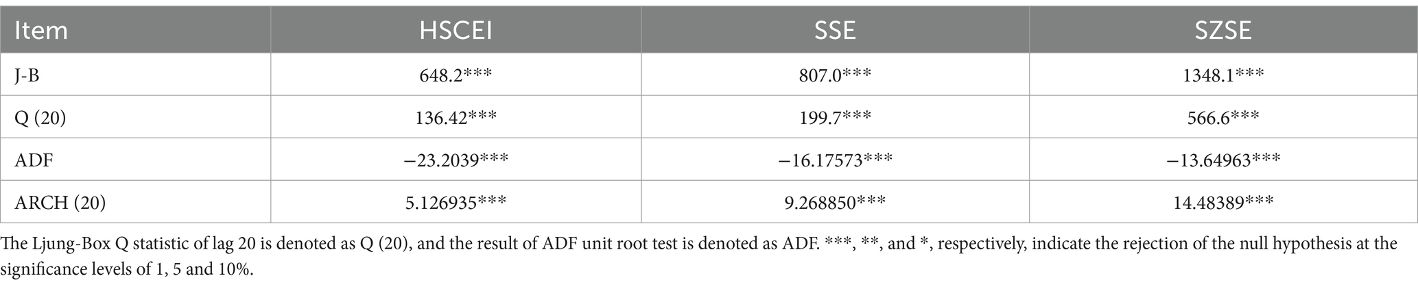
Table 1. Test results.

Using Lagrange multiplier method, we obtained the test results that the p-values of the residual series of the daily return from the 1^st to the 5^th order are all 0 at 5% significance level, indicating that there is a significant ARCH effect in the residual of the daily return.

4.2 Dynamic correlation coefficient

There is a significant serial correlation in the daily return series of all HSCEI, SSE and SZSE based on the correlation test. Therefore, the equation of the AR model was used when constructing the mean equation of the single-variable GARCH model. After multiple comparisons with Eviews, the optimal form of the mean equation is obtained based on the SC minimum principle. This process is illustrated by the following Equations 15–17.

$\begin{array}{ll}{R}_{\mathit{HSCEI},t}=k_t{R}_{\mathit{HSCEI},t-1}+c+e_t& (15)\end{array}$

$\begin{array}{ll}{R}_{SSE,t}=k_1{R}_{SSE,t-1}+k_2{R}_{SSE,t-2}+k_3{R}_{SSE,t-3}+c+e_t& (16)\end{array}$

$\begin{array}{l}{R}_{\mathit{SZSE},t}=k_1{R}_{\mathit{SZSE},t-1}+k_2{R}_{\mathit{SZSE},t-2}+k_3{R}_{\mathit{SZSE},t-3}\\ +k_4{R}_{\mathit{SZSE},t-4}+c+e_t\end{array}\text{ (17)}$

The Ljung-Box Q statistic test was performed on the residual series of the above three equations, and the corresponding p values were relatively large, so the initial hypothesis was accepted, which showed that there was no auto-correlation in these equations. The ARCH test was performed on the residual series, and the results showed that there was a significant ARCH effect in them, which could be further analyzed by building a GARCH model.

Research by Baillie and Bollerslev showed that GARCH (1,1) could well fit the stock market returns volatility, meanwhile with the simplicity as its advantage. Therefore, this paper selected the GARCH (1,1) model to analyze the returns volatility (29). Based on the mean equation of the auto-regressive form that was determined in this section, the GARCH (1,1) model was used to re-fit the returns volatility. The results of the maximum likelihood estimation of the parameters are in Table 2. The estimated results of the parameters in Table 2 show that the estimated value of each parameter is significant, and the value of α + β is close to 1, indicating that the volatility of each stock index has significant persistence.

Table 2

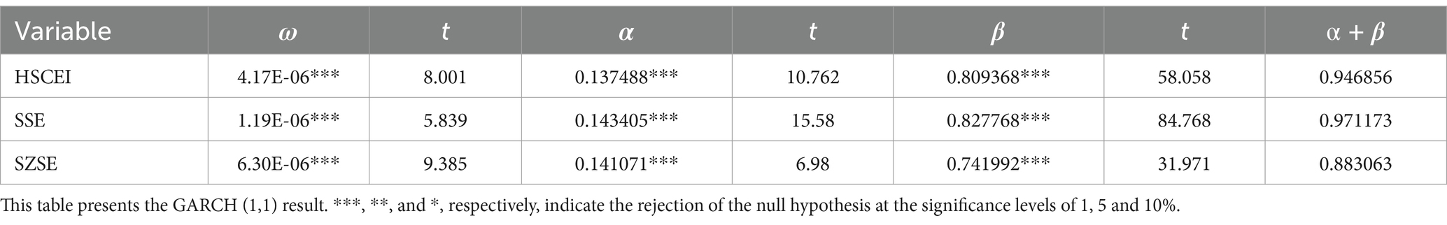
Table 2. GARCH (1,1) result.

This paper used GARCH (1,1) to estimate the standardized mean equation residuals of HSCEI, SSE and SZSE. Based on the dynamic correlation coefficient in the DCC-GARCH model, Figures 1–3 are obtained, where the blue line is the dynamic correlation coefficient of the stock indices and the red line is the COVID-19 transmission rate.

Figure 1

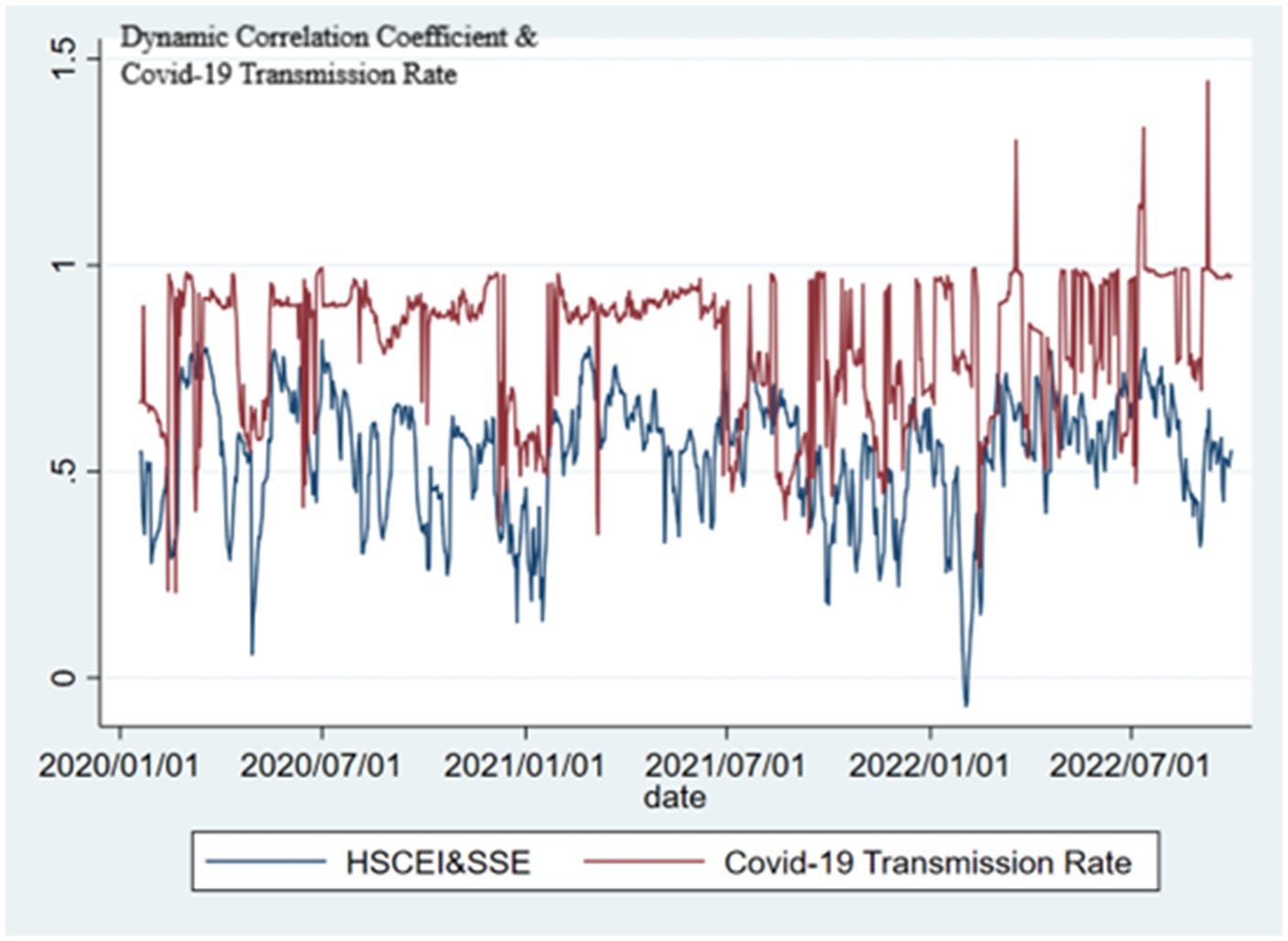
Figure 1. HSCEI&SSE dynamic correlation coefficient.

Figure 2

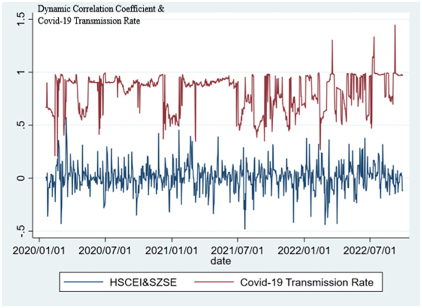
Figure 2. HSCEI&SZSE dynamic correlation coefficient.

Figure 3

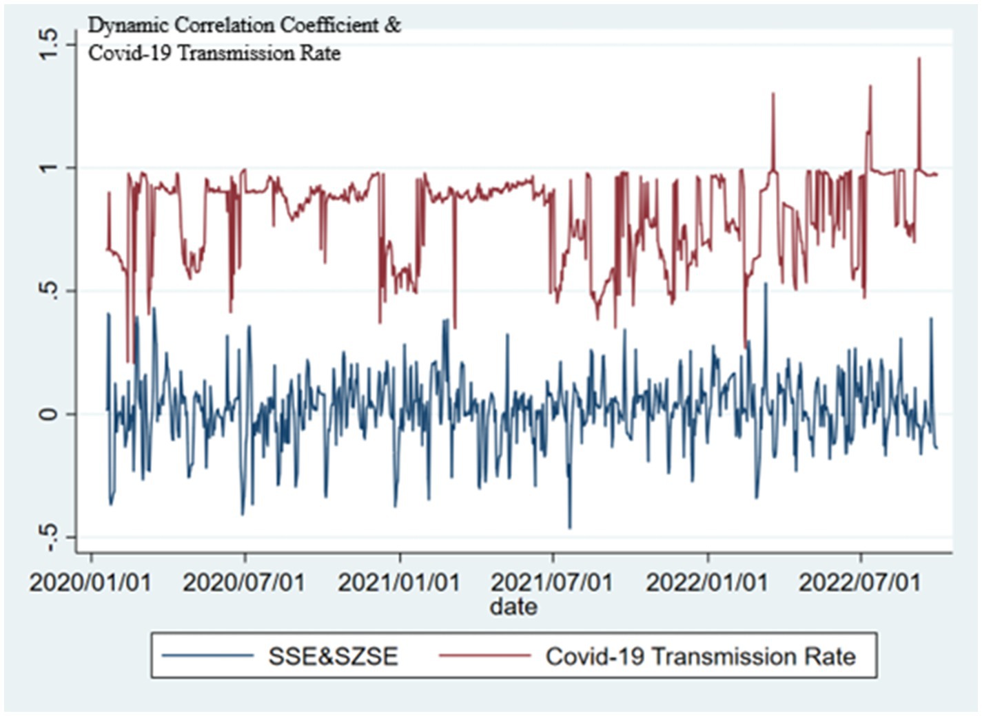
Figure 3. SSE&SZSE dynamic correlation coefficient.

The DCC-GARCH model is used to estimate the correlation coefficient of the daily returns of the HSCEI, SSE and SZSE. Here, the conditional variances are set to the form of GARCH (1,1) and the order of the DCC model is also set to 1. The estimation results are shown in Table 3 that α and β are significantly different from 0, indicating that the lagged period standardized residual value has a significant effect on the dynamic correlation coefficient. α and β have obvious statistical properties that can be used to assess the existence of variable conditional correlation coefficients.

Table 3

Table 3. DCC-GARCH results.

5 Empirical result

5.1 Descriptive statistics

Table 4 shows that the mean of the first-day COVID-19 transmission rate is 0.811, which is less than 1, indicating that the overall COVID-19 transmission in mainland China is under control. However, the maximum is 1.445, indicating that there have been outbreaks of COVID-19 in mainland China in a short term. The mean of the second-day COVID-19 transmission rate is 0.128, and the maximum is 0.792, both of which are less than 1, indicating that in most cases, even if COVID-19 outbreaks occurred in mainland China, they would be quickly contained. Meanwhile, it can be seen from Table 5 that the dynamic correlation between HSCEI&SSE is the strongest, indicating a close connection between Hong Kong stock market and Shanghai stock market, while Shenzhen stock market is relatively independent.

Table 4

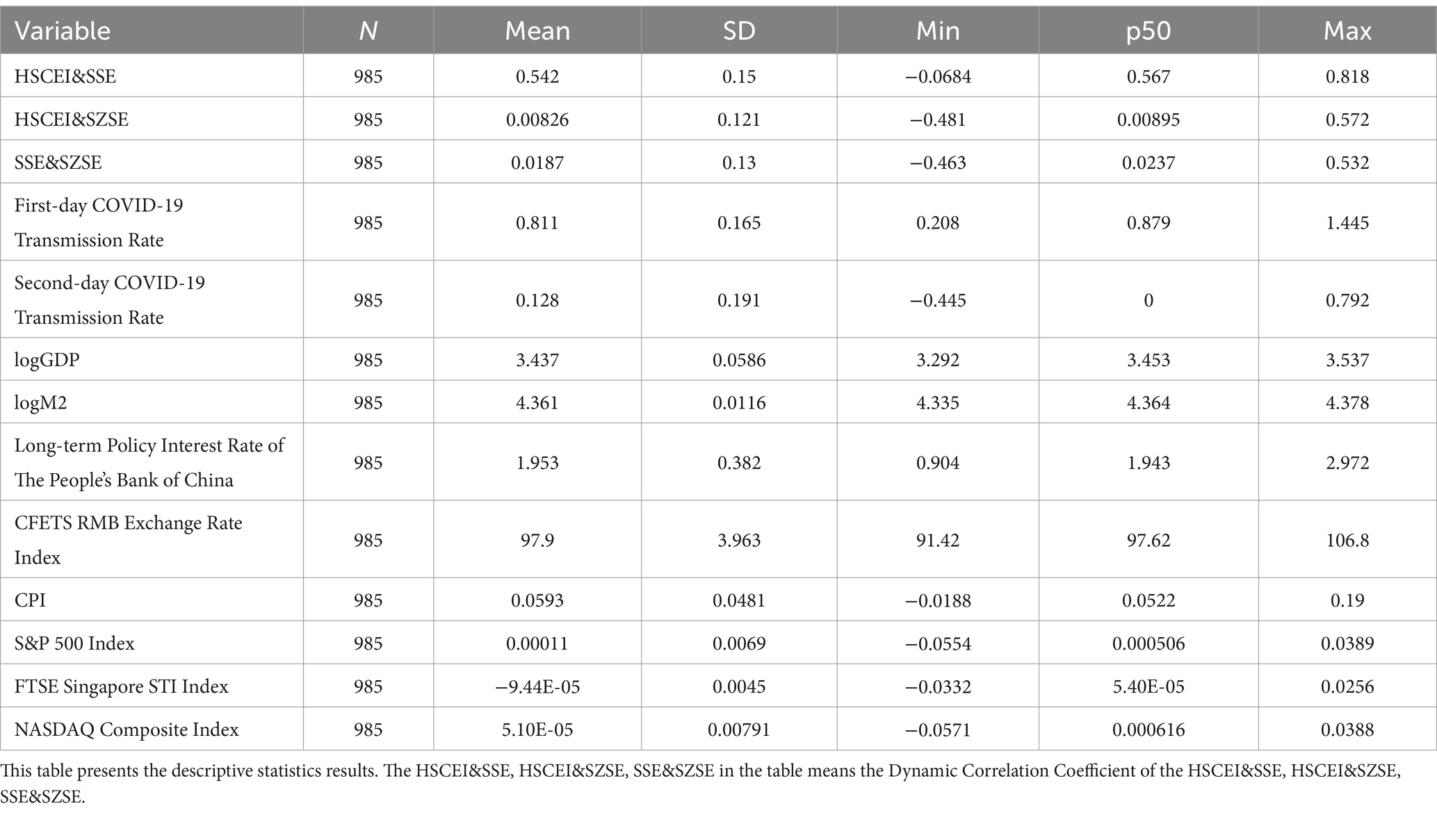
Table 4. Descriptive statistics.

Table 5

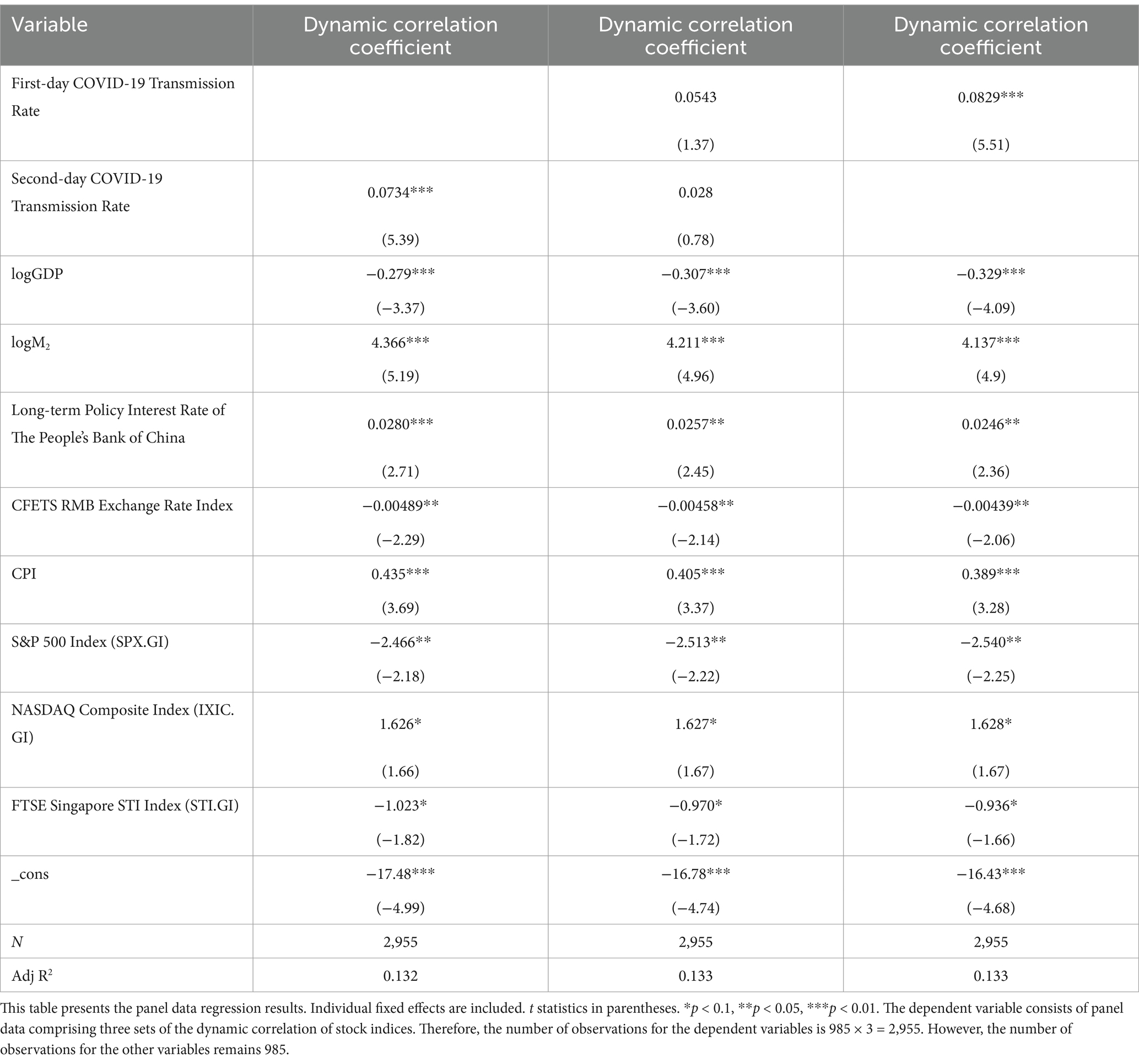
Table 5. Panel data regression result.

5.2 Panel data model regression

The regression results of the panel data model are presented in Table 5.

The results in Table 5 show that there is a significant positive correlation between the dynamic correlation coefficient between stock indices and the COVID-19 transmission rate. This indicates that as the transmission rate of the COVID-19 increases, the correlation between stock indices becomes stronger; conversely, as the transmission rate decreases, the correlation weakens.

It is noteworthy that when both the first-day COVID-19 transmission rate and the second-day COVID-19 transmission rate are included as independent variables, the regression results obtained are not significant. The reason for this outcome is that there exists a certain correlation between the first-day COVID-19 transmission rate and the second-day COVID-19 transmission rate, and when they are both used as independent variables, they can influence each other.

6 Robustness test

6.1 OLS model regression

In this paper, the three group of the dynamic correlation of stock indices is taken as the dependent variables respectively, and an OLS model is established for regression analysis. In this section, the selected control variables remain unchanged. The regression results of the model are presented in Tables 6–8.

Table 6

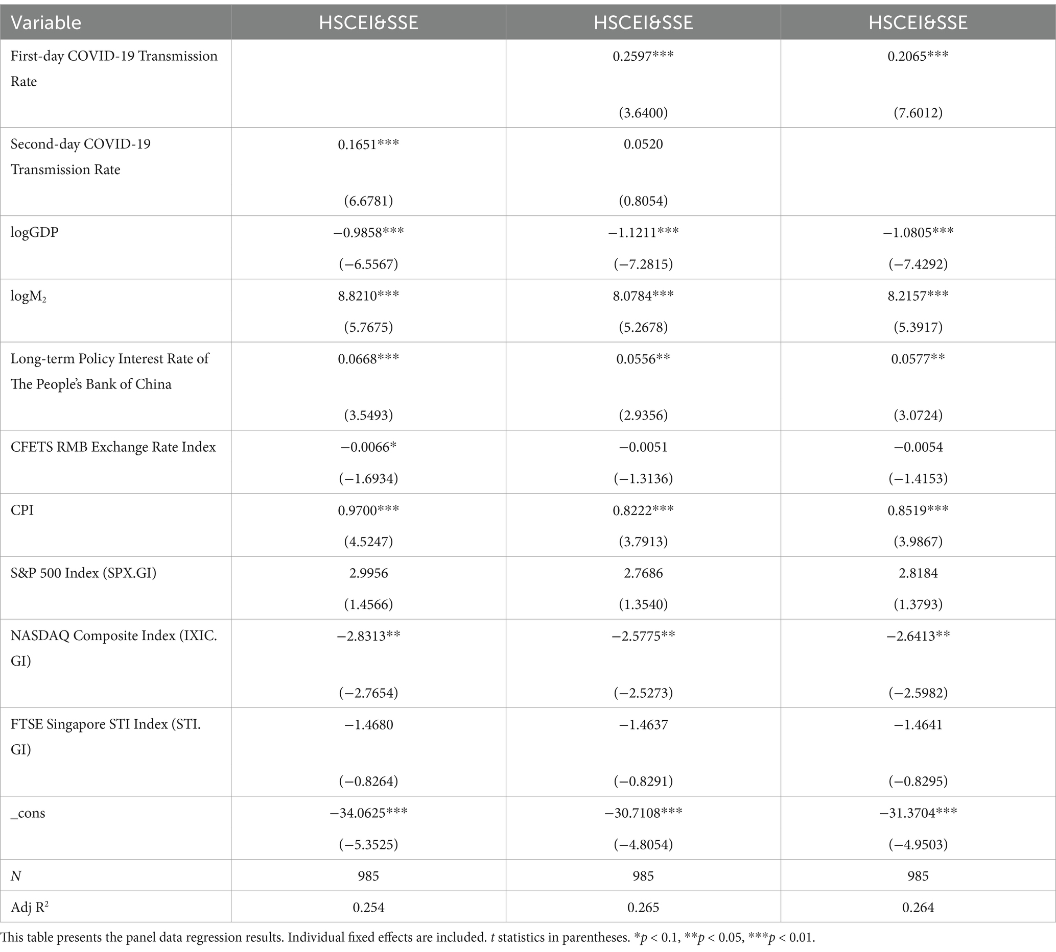
Table 6. HSCEI&SSE regression result.

Table 7

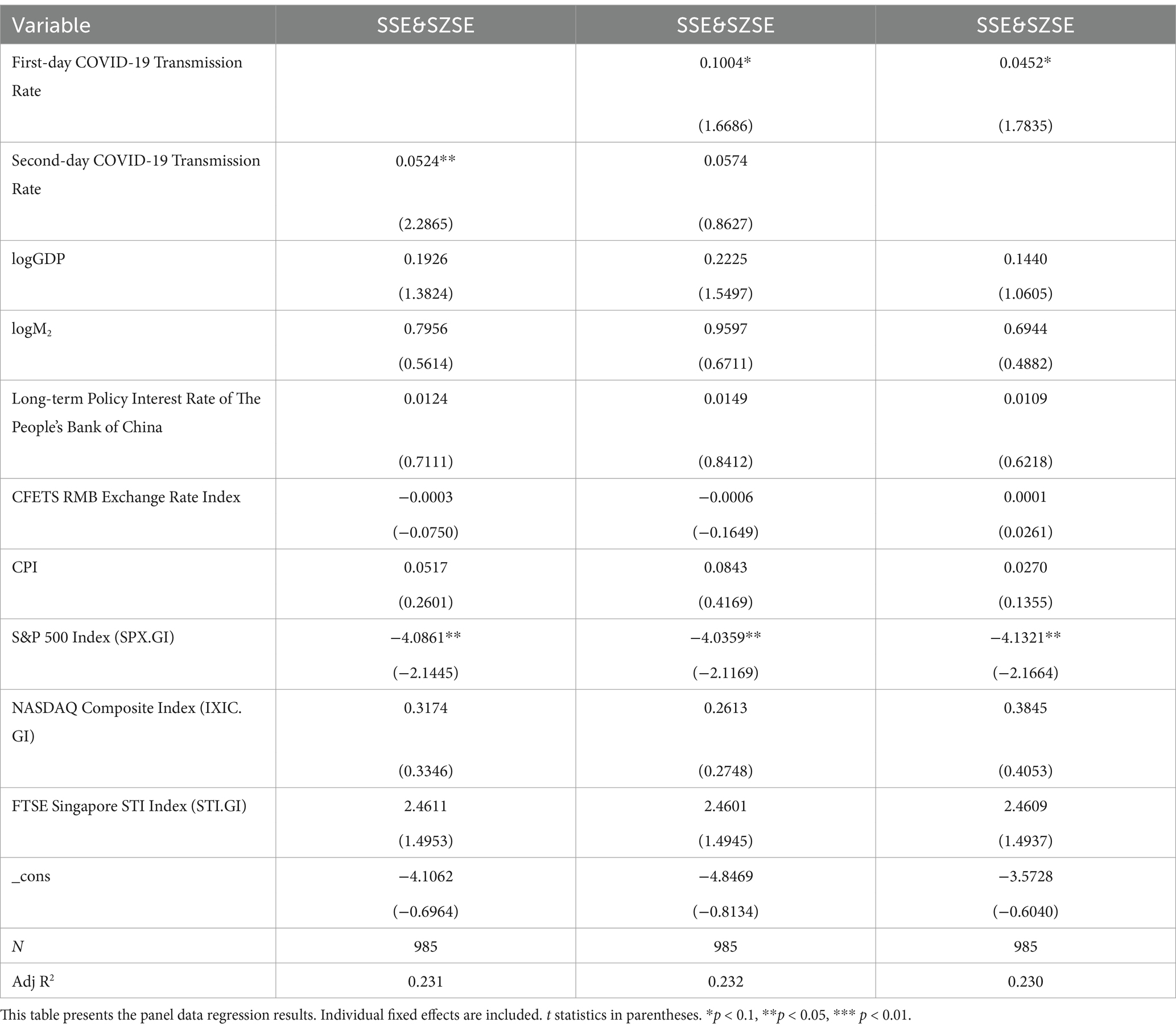
Table 7. SSE&SZSE regression result.

Table 8

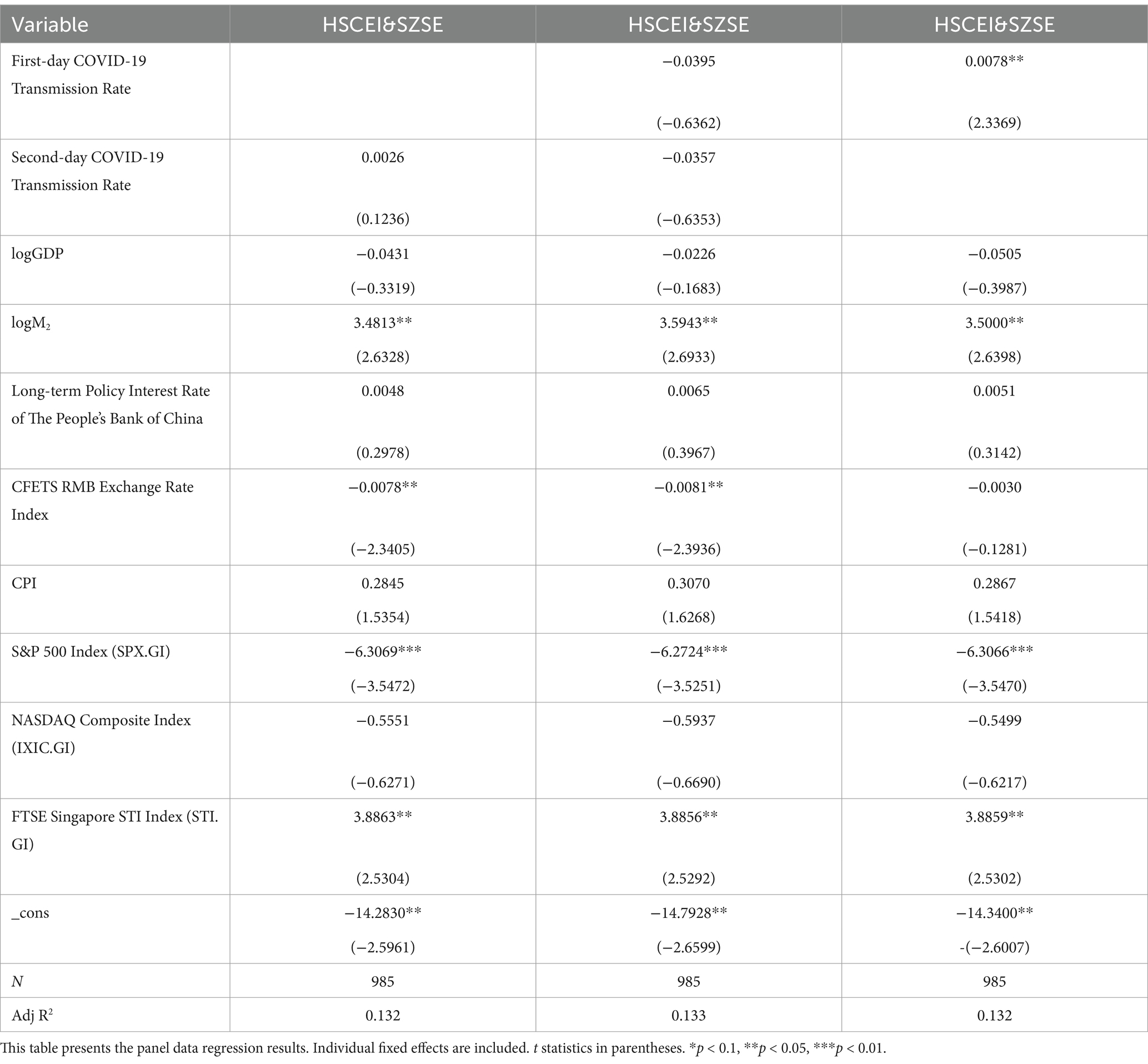
Table 8. HSCEI&SZSE regression result.

Table 6 shows that there is a significant positive correlation between the First-day COVID-19 Transmission Rate and the dynamic correlation coefficient of HSCEI&SSE, and similarly, there is also a significant positive correlation between the Second-day COVID-19 Transmission Rate and the dynamic correlation coefficient of HSCEI&SSE.

Table 7 reveals a significant positive correlation between the First-day COVID-19 Transmission Rate and the dynamic correlation coefficient of SSE&SZSE. Additionally, a significant positive correlation is also observed between the Second-day COVID-19 Transmission Rate and the dynamic correlation coefficient of HSCEI&SSE.

Table 8 demonstrates a significant positive correlation between the First-day COVID-19 Transmission Rate and the dynamic correlation coefficient of HSCEI&SZSE. However, no significant correlation is found between the Second-day COVID-19 Transmission Rate and the dynamic correlation coefficient of HSCEI&SSE.

In summary, the First-day COVID-19 Transmission Rate demonstrates a significant positive correlation with the dynamic correlation coefficient of HSCEI&SSE, SSE&SZSE, and HSCEI&SZSE, respectively. This finding aligns with the results from the empirical testing section of this paper. The Second-day COVID-19 Transmission Rate, on the other hand, shows no correlation with the dynamic correlation coefficient of HSCEI&SZSE, but exhibits a significant positive correlation with the dynamic correlation coefficient of HSCEI&SSE and SSE&SZSE.

This indicates that the COVID-19 pandemic has increased the co-movements among stock markets. In other words, the outbreak of COVID-19 can be viewed as a systemic risk, prompting Chinese investors to sell their stocks and hold cash as a means of risk aversion in response to the outbreak. Nevertheless, once the outbreak is brought under control, these investors would reinvest their cash holdings back into the stock market, causing a synchronized rise and fall across different stock markets during the COVID-19 pandemic. This article believes that this is the reason why the three co-movements react in the same manner to the COVID-19 transmission rate fluctuations.

Furthermore, the coefficients of the COVID-19 transmission rate presented in Table 7 (SSE & SZSE) and Table 8 (HSCEI & SZSE) are significantly smaller than those in Table 6 (HSCEI & SSE). This paper attributes this phenomenon to the significantly higher proportion of pharmaceutical stocks in the SZSE compared to the SSE and HSCEI. During the COVID-19 pandemic, pharmaceutical stocks exhibited an upward trend, resulting in a lower degree of co-movement between SZSE and either SSE or HSCEI compared to the co-movement between SSE and HSCEI.

To sum up, we can conclude that the results of the robustness test still indicate that an increase in the COVID-19 transmission rate reinforced the dynamic correlation coefficient of stock indices, which passed the robustness test.

6.2 Government intervention and public opinion

There was evidence that the government intervention (30) and the public opinion (31), related to COVID-19, had influenced co-movement among stock markets during the COVID-19 pandemic, so this paper incorporates these two elements as additional control variables in the panel data model regression (15). Considering that government intervention and public opinion are not in quantitative form, so they need to be quantified.

Drawing on the quantification method for public opinion proposed by Chang et al. and Chen et al., and the quantification method for government intervention proposed by Diepeveen et al., and considering China’s conditions at that time, the quantification method utilized in this paper is as follows. First, Baidu Index, the index of the largest search engine within mainland China, is selected as the data source, which is used to reflect the times that the words or the sentences containing these words were searched for on a given day. Then the Baidu Index of the keywords related to government intervention and public opinion are used to indicate the attention to government intervention and daily public opinion on COVID-19 (32–34).

This paper selects five keywords related to COVID-19 to assess the public opinion during the COVID-19 pandemic, namely, the Chinese characters for COVID-19, COVID-19, the Chinese characters for DAILY NEW CONFIRMED CASES, the Chinese characters for VIRUS, and the Chinese characters for DEATHS, and another five keywords related to COVID-19 to assess the government intervention during the COVID-19 pandemic, namely, the Chinese characters for LOCKDOWN, the Chinese characters for MAKESHIFT HOSPITAL, the Chinese characters for HEALTH CODE, the Chinese characters for COVID-19 TESTING, and the Chinese characters for GOVERNMENT INTERVENTION.

The multicollinearity test reveals that the Baidu Index for the five keywords which represent the COVID-19 related public opinion exhibit multicollinearity. Similarly, the Baidu Index for the five keywords which represent the COVID-19 related government intervention also show multicollinearity. To tackle this issue, the method of principal components analysis (PCA) is employed to eliminate such multicollinearity, creating two composite variables, one representing the COVID-19 related public opinion and the other representing the COVID-19 related government intervention. Subsequently, the multicollinearity tests on these two composite variables, along with all the other control variables and the explanatory variable (the dynamic COVID-19 Transmission Rate) reveal that no multicollinearity is found (35, 36).

The regression results are shown in Table 9.

Table 9

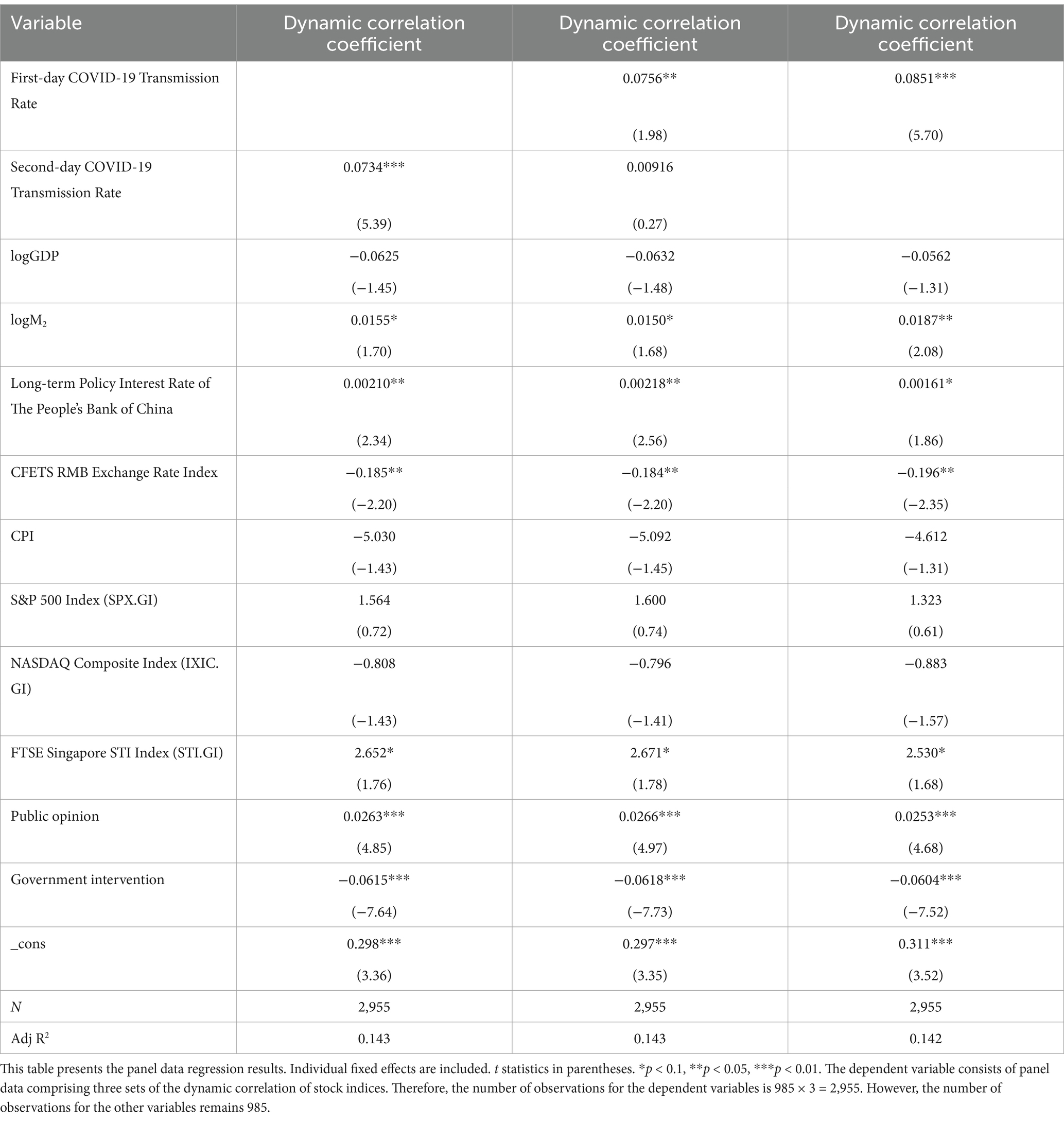
Table 9. Panel data regression result (including government intervention and public opinion).

Table 9 shows that although adding these two control variables, which represent the COVID-19 related government intervention and the COVID-19 related public opinion, the regression coefficient of the dynamic COVID-19 transmission rate remains significant. Meanwhile, when both the First-day and the Second-day COVID-19 transmission rate are used as explanatory variables concurrently, the regression coefficient of the First-day rate appears significant. In contrast, the regression analyses in Section 5 reveal that the regression coefficients of both are insignificant. Therefore, the inclusion of the COVID-19 related public opinion and government intervention as control variables justifies.

Table 9 shows that the COVID-19 related public opinion has a positive regression coefficient, while the COVID-19 related government intervention has a negative one. This is because the enhancement in public opinion often accompanies epidemic spread, while more government intervention tends to contain it. The spread of the epidemic generally leads to the declines of the stock prices, increasing co-movement of stock markets. However, as the epidemic is brought under control, market responses diverge based on regional economic conditions, policy interventions, and sectoral resilience, leading to varied recovery speeds and degrees. This divergence diminishes synchronized market movements, thereby reducing overall co-movement of stock markets. This also helps explain why the regression coefficient of the dynamic COVID-19 transmission rate is positive.

6.3 Lag effects

This paper holds that the impact of the dynamic COVID-19 transmission rate on co-movement among stock markets has lag effects. Therefore, this paper introduces 1-day, 5-day, and 7-day lags for the original explanatory variables, specifically the First-day COVID-19 Transmission Rate and the Second-day COVID-19 Transmission Rate. These lagged variables are subsequently used for the regression of the panel data model. The regression results are presented in Table 10.

Table 10

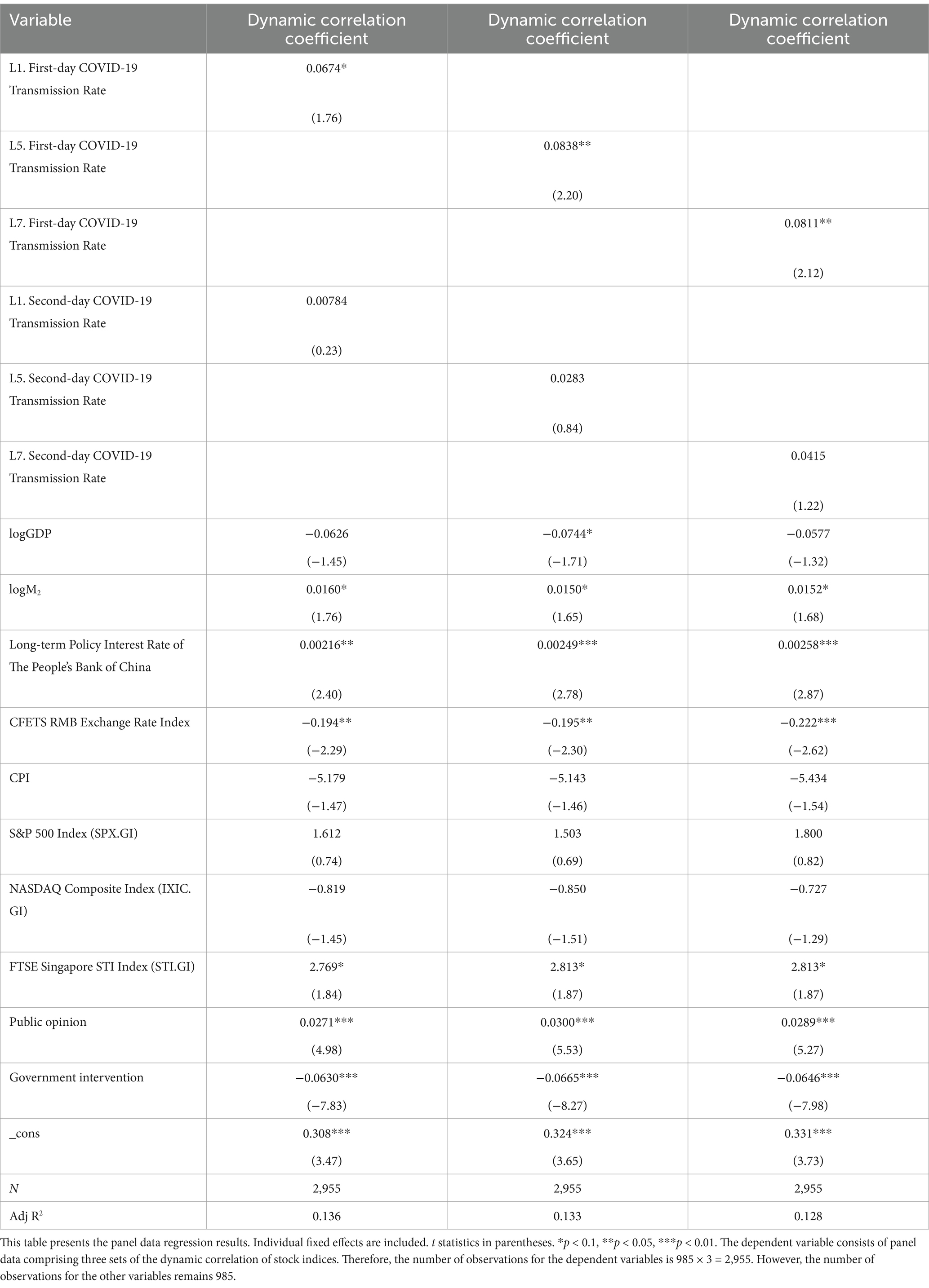
Table 10. Panel data regression results related to lag effects.

Table 10 shows that the coefficient for the First-day COVID-19 Transmission Rate lagged by 1, 5, and 7 days, are all significant. This means the dynamic COVID-19 transmission rate affects co-movement among stock markets not only in the short-term period but also in the long-term, with the effect persisting for over 1 week.

Further, the regression coefficient for the First-day COVID-19 Transmission Rate lagged by 10 days remains significant. When the lag extends to 11 days, the coefficient becomes insignificant. The results are detailed in Table A1 in Appendix 4.

7 Discussion

This paper holds that the dynamic transmission rate and the number of daily new confirmed COVID-19 cases both can serve as key variables describing the COVID-19 pandemic. However, as mentioned in the “Introduction” section, when the number of daily new confirmed COVID-19 cases are used as an explanatory variable, the results of regression analysis indicate no significant correlation between the number of these cases and co-movement of stock markets.

For the lack of significant correlation between the number of daily new confirmed COVID-19 cases and co-movement of stock markets, this paper proposes the following explanations: first, the dynamic transmission rate may be influenced by both external factors (e.g., government intervention, public opinion) and internal factors (e.g., virus mutation); second, the number of daily new confirmed cases may depend not only on the external and internal factors mentioned above, but also on the number of new confirmed cases in the previous period. In addition, from a theoretical standpoint, the number of new confirmed cases in the previous period should not affect the co-movement of the current stock markets. Two simulation scenarios are designed for further explanation.

Scenario 1: Suppose that both the government intervention and the public opinion keep stable and virus strain remain unchanged, and then the co-movement of stock markets would be unlikely to change significantly. Under a transmission rate of 1.1, if there are 100 new confirmed cases on Day t, the number of new confirmed cases would rise to 110 on Day t + 1, a 10-case increase from Day t. Similarly, the number would increase to 121 on Day t + 2, an 11-case rise from Day t + 1.

The regression coefficient of the explanatory variable in the regression equation is assumed to be k. When the COVID-19 dynamic transmission rate serves as the explanatory variable, the co-movement of the stock markets calculated from the regression equation will not change significantly, because during Day t to Day t + 2, the COVID-19 dynamic transmission rate does not change. However, when the daily number of new confirmed cases are used as the explanatory variable, the co-movement of the stock markets calculated from the regression equation will increase by 10 k on Day t + 1, and then it will increase by another 11 k on Day t + 2.

Based on the aforementioned analysis, this paper argues that utilizing the dynamic transmission rate of COVID-19 as an explanatory variable to describe the COVID-19 pandemic in regression model can better capture the pandemic’s impact on co-movement of stock markets.

Scenario 2: Suppose that both the government intervention and the public opinion keep stable and virus strain remain unchanged, and then the co-movement of stock markets would be unlikely to change significantly. Under a transmission rate of 0.9, if there are 100 new confirmed cases on Day t, the number of new confirmed cases will reduce to 90 on Day t + 1, a 10-case decrease from Day t. Similarly, the number would reduce to 81 on Day t + 2, down by 9 from Day t + 1.

The regression coefficient of the explanatory variable in the regression equation is assumed to be k. When the COVID-19 dynamic transmission rate serves as the explanatory variable, the co-movement of the stock markets calculated from the regression equation will not change significantly, because during Day t to Day t + 2, the COVID-19 dynamic transmission rate does not change. However, when using the number of daily new confirmed cases as the explanatory variable, the co-movement of the stock markets calculated from the regression equation will decrease by 10 k on Day t + 1, and then it will decrease by another 9 k on Day t + 2.

Based on the aforementioned analysis, this paper argues that utilizing the dynamic transmission rate of COVID-19 as an explanatory variable to describe the COVID-19 pandemic in regression model can better capture the pandemic’s impact on co-movement of stock markets.

To sum up, the analysis of Scenario1 and 2 reveals that the dynamic transmission rate of COVID-19 is timelier in reflecting the spread of COVID-19 than the number of daily new confirmed cases. It avoids the issue of having to consider the previous period’s confirmed cases. Therefore, using the dynamic transmission rate of COVID-19 as the explanatory variable allows for a more in-depth exploration on the relationship between the COVID-19 pandemic and co-movement of stock markets, which can also explain why there is no significant relationship between the number of daily new confirmed COVID-19 cases and co-movements of stock markets.

8 Conclusion

From 2020 to 2023, the COVID-19 pandemic swept across the globe, during which, the impact of COVID-19 on stock markets emerged as a key area of research. Many studies investigated the effects of the pandemic on stock prices and returns. However, research on how COVID-19 influences the co-movement of stock markets is still limited. To address this gap, this paper delves into the impact of the COVID-19 transmission rate on the co-movement of China’s stock markets.

This study examines three stock indices: HSCEI, SSE, and SZSE. We employ a DCC-GARCH model to calculate the dynamic correlation coefficients between these indices, specifically HSCEI&SSE, HSCEI&SZSE, and SSE&SZSE, designating them as dependent variables. Furthermore, we utilize the model developed by Xiao et al. to assess the dynamic transmission rate of COVID-19 in China, which serves as the independent variable in our analysis.

To be further clarified, we select the dynamic COVID-19 transmission rate as the independent variable in our study, rather than the number of new confirmed cases, because our findings suggest that new confirmed cases do not significantly impact the co-movement of stock markets, contradicting our initial hypothesis. This may also explain why previous researchers have been hesitant to explore the impact of the COVID-19 pandemic on stock market co-movement, for co-movement among stock markets is influenced not only by the number of new confirmed cases but also by government pandemic prevention policies, and quantifying the government pandemic prevention policies properly is not an easy job. Therefore, this paper adopts the method of calculating the dynamic COVID-19 transmission rate, as proposed by Xiao et al., which incorporates both fluctuations in the number of new confirmed cases during the pandemic and the government’s pandemic prevention policies (8).

Our empirical results ultimately demonstrate a significant positive correlation between the dynamic COVID-19 transmission rate and the dynamic correlation coefficient between stock indices, indicating that COVID-19 pandemic increased co-movement among China’s stock markets. Conversely, effective containment of COVID-19 pandemic reduced co-movement among China’s stock markets. This paper innovatively selects the dynamic transmission rate of COVID-19 as the independent variable, providing a novel approach for subsequent studies on the impact of COVID-19 and other PHEIC events.

Therefore, for investors in stock markets, during a PHEIC event, attempting to diversify risk by investing funds into different stock markets is ineffective. The way to reduce losses from a PHEIC event is to sell the held stocks. For governments, in the event of a PHEIC, it is necessary to promptly introduce effective pandemic prevention measures. This can not only reduce confirmed cases and deaths but also mitigate the impact of the PHEIC event on domestic financial markets, stabilizing the development of domestic financial markets.

Data availability statement

SSE, SZSE, HSI, SPX.GI, IXIC.GI, STI.GI, GDP, M₂, Long-term Policy Interest Rate of The People’s Bank of China, CFETS RMB Exchange Rate Index, and CPI are from the Wind database; Government Intervention and Public Opinion data are from Baidu Index; COVID-19 confirmed cases data are from the World Health Organization, and the specific link is https://data.who.int/dashboards/covid19/data.

Author contributions

HX: Conceptualization, Data curation, Formal analysis, Funding acquisition, Investigation, Methodology, Project administration, Resources, Software, Supervision, Validation, Visualization, Writing – original draft, Writing – review & editing. DL: Data curation, Formal analysis, Validation, Writing – review & editing. ZZ: Investigation, Validation, Visualization, Writing – review & editing.

Funding

The author(s) declare that no financial support was received for the research and/or publication of this article.

Acknowledgments

The authors wish to express their sincere thanks to the City University of Macau for its support and assistance in this study.

Conflict of interest

HX was employed by Shenwan Hongyuan Securities Co., Ltd.

The remaining authors declare that the research was conducted in the absence of any commercial or financial relationships that could be construed as a potential conflict of interest.

Generative AI statement

The authors declare that no Gen AI was used in the creation of this manuscript.

Publisher’s note

All claims expressed in this article are solely those of the authors and do not necessarily represent those of their affiliated organizations, or those of the publisher, the editors and the reviewers. Any product that may be evaluated in this article, or claim that may be made by its manufacturer, is not guaranteed or endorsed by the publisher.

Supplementary material

The Supplementary material for this article can be found online at: https://www.frontiersin.org/articles/10.3389/fams.2025.1564664/full#supplementary-material

References

1. Sohrabi, C, Alsafi, Z, O’neill, N, Khan, M, Kerwan, A, Al-Jabir, A, et al. World Health Organization declares global emergency: a review of the 2019 novel coronavirus (COVID-19). Int J Surg. (2020) 76:71–6. doi: 10.1016/j.ijsu.2020.02.034

PubMed Abstract | Crossref Full Text | Google Scholar

2. Hao, R, Zhang, Y, Cao, Z, Li, J, Xu, Q, Ye, L, et al. Control strategies and their effects on the COVID-19 pandemic in 2020 in representative countries. J Biosaf Biosecur. (2021) 3:76–81. doi: 10.1016/j.jobb.2021.06.003

PubMed Abstract | Crossref Full Text | Google Scholar

3. Yang, ZH, Chen, YT, and Zhang, PM. Macroeconomic shock, financial risk transmission and governance response to major public emergencies. Manage World. (2020) 36:13–35. doi: 10.19744/j.cnki.11-1235/f.2020.0067

Crossref Full Text | Google Scholar

4. He, Q, Liu, J, Wang, S, and Yu, J. The impact of COVID-19 on stock markets. Econ Polit Stud. (2020) 8:275–88. doi: 10.1080/20954816.2020.1757570

Crossref Full Text | Google Scholar

5. Al-Awadhi, AM, Alsaifi, K, Al-Awadhi, A, and Alhammadi, S. Death and contagious infectious diseases: impact of the COVID-19 virus on stock market returns. J Behav Exp Financ. (2020) 27:100326. doi: 10.1016/j.jbef.2020.100326

PubMed Abstract | Crossref Full Text | Google Scholar

6. Ashraf, BN. Economic impact of government interventions during the COVID-19 pandemic: international evidence from financial markets. J Behav Exp Financ. (2020) 27:100371. doi: 10.1016/j.jbef.2020.100371

PubMed Abstract | Crossref Full Text | Google Scholar

7. Ashraf, BN. Stock markets’ reaction to Covid-19: moderating role of national culture. Financ Res Lett. (2021) 41:101857. doi: 10.1016/j.frl.2020.101857

PubMed Abstract | Crossref Full Text | Google Scholar

8. Xiao, H, Lin, D, and Li, S. Novel method for estimating time-varying COVID-19 transmission rate. Mathematics. (2023) 11:2383. doi: 10.3390/math11102383

Crossref Full Text | Google Scholar

9. Johnson, TF, Hordley, LA, Greenwell, MP, and Evans, LC. Associations between COVID-19 transmission rates, park use, and landscape structure. Sci Total Environ. (2021) 789:148123. doi: 10.1016/j.scitotenv.2021.148123

PubMed Abstract | Crossref Full Text | Google Scholar

10. Carleton, T., and Meng, K. C. (2020). Causal empirical estimates suggest COVID-19 transmission rates are highly seasonal. MedRxiv, 2020–2003.

Google Scholar

11. Mahmoudi, MR, Baleanu, D, Mansor, Z, Tuan, BA, and Pho, KH. Fuzzy clustering method to compare the spread rate of COVID-19 in the high risks countries. Chaos Solitons Fractals. (2020) 140:110230. doi: 10.1016/j.chaos.2020.110230

PubMed Abstract | Crossref Full Text | Google Scholar

12. Samui, P, Mondal, J, and Khajanchi, S. A mathematical model for COVID-19 transmission dynamics with a case study of India. Chaos Solitons Fractals. (2020) 140:110173. doi: 10.1016/j.chaos.2020.110173

PubMed Abstract | Crossref Full Text | Google Scholar

13. Mbuvha, R, and Marwala, T. Bayesian inference of COVID-19 spreading rates in South Africa. PLoS One. (2020) 15:e0237126. doi: 10.1371/journal.pone.0237126

PubMed Abstract | Crossref Full Text | Google Scholar

14. Dharmaratne, S, Sudaraka, S, Abeyagunawardena, I, Manchanayake, K, Kothalawala, M, and Gunathunga, W. Estimation of the basic reproduction number (R0) for the novel coronavirus disease in Sri Lanka. Virol J. (2020) 17:1–7. doi: 10.1186/s12985-020-01411-0

PubMed Abstract | Crossref Full Text | Google Scholar

15. Zehri, C. Stock market comovements: evidence from the COVID-19 pandemic. J Econ Asymmetries. (2021) 24:e00228. doi: 10.1016/j.jeca.2021.e00228

PubMed Abstract | Crossref Full Text | Google Scholar

16. Cheng, H, and Glascock, JL. Dynamic linkages between the greater China economic area stock markets—mainland China, Hong Kong, and Taiwan. Rev Quant Finan Acc. (2005) 24:343–57. doi: 10.1007/s11156-005-7017-7

Crossref Full Text | Google Scholar

17. Carausu, D. N., and Lupu, D. (2022). COVID-19 and stock markets comovement in emerging Europe. In Proceedings of the International Conference on Business Excellence (Vol. 16, No. 1, pp. 660–669).

Google Scholar

18. Ali, S, Naveed, M, Saleem, A, and Nasir, MW. Time-frequency co-movement between COVID-19 and Pakistan’s stock market: empirical evidence from wavelet coherence analysis. Ann Finan Econ. (2022) 17:2250026. doi: 10.1142/S2010495222500269

Crossref Full Text | Google Scholar

19. Junior, PO, Tetteh, JE, Nkrumah-Boadu, B, and Adjei, AN. Comovement of African stock markets: any influence from the COVID-19 pandemic? Heliyon. (2024) 10. doi: 10.1016/j.heliyon.2024.e29409

Crossref Full Text | Google Scholar

20. Verma, R. Comovement of stock markets pre-and post-COVID-19 pandemic: a study of Asian markets. IIM Ranchi J Manage Stud. (2024) 3:25–38. doi: 10.1108/IRJMS-09-2022-0086

Crossref Full Text | Google Scholar

21. Phiri, A, Anyikwa, I, and Moyo, C. Co-movement between COVID-19 and G20 stock market returns: a time and frequency analysis. Heliyon. (2023) 9:e14195. doi: 10.1016/j.heliyon.2023.e14195

PubMed Abstract | Crossref Full Text | Google Scholar

22. Huang, W, Wang, H, Wei, Y, and Chevallier, J. Complex network analysis of global stock market co-movement during the COVID-19 pandemic based on intraday open-high-low-close data. Financ Innov. (2024) 10:1–50. doi: 10.1186/s40854-023-00548-5

PubMed Abstract | Crossref Full Text | Google Scholar

23. Engle, RF. Autoregressive conditional heteroscedasticity with estimates of the variance of United Kingdom inflation. Econometrica. (1982) 50:987–1007. doi: 10.2307/1912773

Crossref Full Text | Google Scholar

24. Bollerslev, T. Generalized autoregressive conditional heteroskedasticity. J Econ. (1986) 31:307–27. doi: 10.1016/0304-4076(86)90063-1

Crossref Full Text | Google Scholar

25. Bollerslev, T, Engle, RF, and Wooldridge, JM. A capital asset pricing model with time-varying covariances. J Polit Econ. (1988) 96:116–31. doi: 10.1086/261527

Crossref Full Text | Google Scholar

26. Engle, R. New frontiers for ARCH models. J Appl Econ. (2002) 17:425–46. doi: 10.1002/jae.683

Crossref Full Text | Google Scholar

27. Ashraf, BN. Stock markets’ reaction to COVID-19: cases or fatalities? Res Int Bus Financ. (2020) 54:101249. doi: 10.1016/j.ribaf.2020.101249

PubMed Abstract | Crossref Full Text | Google Scholar

28. Feng, GF, Yang, HC, Gong, Q, and Chang, CP. What is the exchange rate volatility response to COVID-19 and government interventions? Econ Anal Policy. (2021) 69:705–19. doi: 10.1016/j.eap.2021.01.018

Crossref Full Text | Google Scholar

29. Baillie, RT, and Bollerslev, T. Prediction in dynamic models with time-dependent conditional variances. J Econometrics. (1992) 52:91–13.

Google Scholar

30. Yang, C, Abedin, MZ, Zhang, H, Weng, F, and Hajek, P. An interpretable system for predicting the impact of COVID-19 government interventions on stock market sectors. Ann Oper Res. (2023):1–28. doi: 10.1007/s10479-023-05311-8

PubMed Abstract | Crossref Full Text | Google Scholar

31. Nian, R, Xu, Y, Yuan, Q, Feng, C, and Lendasse, A. Quantifying time-frequency co-movement impact of COVID-19 on US and China stock market toward investor sentiment index. Front Public Health. (2021) 9:727047. doi: 10.3389/fpubh.2021.727047

PubMed Abstract | Crossref Full Text | Google Scholar

32. Chang, Y. C., Lee, F. Y., and Chen, C. H. (2018). A public opinion keyword vector for social sentiment analysis research. In 2018 tenth international conference on advanced computational intelligence (ICACI) (pp. 752–757). IEEE.

Google Scholar

33. Chen, L, Liu, Y, Chang, Y, Wang, X, and Luo, X. Public opinion analysis of novel coronavirus from online data. J Safety Sci Resilience. (2020) 1:120–7. doi: 10.1016/j.jnlssr.2020.08.002

Crossref Full Text | Google Scholar

34. Diepeveen, S, Ling, T, Suhrcke, M, Roland, M, and Marteau, TM. Public acceptability of government intervention to change health-related behaviours: a systematic review and narrative synthesis. BMC Public Health. (2013) 13:1–11. doi: 10.1186/1471-2458-13-756

PubMed Abstract | Crossref Full Text | Google Scholar

35. Maćkiewicz, A, and Ratajczak, W. Principal components analysis (PCA). Comput Geosci. (1993) 19:303–42. doi: 10.1016/0098-3004(93)90090-R

Crossref Full Text | Google Scholar

36. Groth, D, Hartmann, S, Klie, S, and Selbig, J. Principal components analysis. Comput Toxicol. (2013) 930:527–47. doi: 10.1007/978-1-62703-059-5_22

Crossref Full Text | Google Scholar