Dynamics and stability of a within-host HIV-HBV co-infection model with time delays

Human immunodeficiency virus (HIV) and hepatitis B virus (HBV) co-infection is common due to their shared transmission routes. Understanding their interaction within host cells is key to improving treatment strategies. Mathematical models are crucial tools for analyzing within-host viral dynamics and informing therapeutic interventions. This study presents a mathematical framework designed to investigate the interactions and progression of HIV-HBV co-infection within a host. The model captures the distinct biological characteristics of the two viruses: HBV primarily infects liver cells (hepatocytes), while HIV targets CD4⁺ T cells and can also infect hepatocytes. A system of seven non-linear delay differential equations (DDEs) is formulated to represent the dynamic interactions among uninfected and virus-infected hepatocytes, uninfected and HIV-infected CD4⁺T cells, as well as circulating HIV and HBV particles. The model incorporates two biologically significant time delays: the first represents the latency between the initial infection and the onset of productive infection in host cells, while the second accounts for the maturation duration of newly produced virions before they become infectious. The model's mathematical consistency is verified by showing that its solutions remain bounded and non-negative throughout the system's dynamics. Equilibrium points and their associated threshold parameters are identified, with conditions for existence and stability rigorously derived. Global stability of the equilibria is established through the application of carefully designed Lyapunov functionals in conjunction with Lyapunov-LaSalle asymptotic stability theorem, ensuring a rigorous and comprehensive analysis of the system's long-term behavior. The theoretical findings are corroborated by numerical simulations. We conducted a sensitivity analysis of the basic reproduction numbers, R₀ for HIV and R₁ for HBV. The effects of antiviral treatment and time delays on the HIV-HBV co-dynamics are discussed. Minimum efficacy thresholds for anti-HIV and anti-HBV therapies are Determined, and when drug effectiveness surpasses these levels, the model predicts the full elimination of both viruses from the host. Additionally, the length of the time delay interval plays a role similar to that of antiviral treatment, suggesting a potential strategy for developing drug therapies aimed at extending the time delay period. The results of this study highlight the importance of incorporating time delays in models of dual viral infection and support the development of treatment strategies that enhance therapeutic outcomes by extending these delays.

1 Introduction

Two deadly viruses for the human body are the human immunodeficiency virus (HIV) and hepatitis B virus (HBV). In several patients, co-infection with these two viruses occurs because they share common transmission routes, such as blood transfusions, use of contaminated syringes, unprotected sexual intercourse, and others [1]. It is estimated that 8% to 10% of people diagnosed with HIV are also infected with HBV worldwide, making it important to study the co-infection of these two viruses. The co-infection with both viruses may increase the symptoms of each disease. This is due to the weakening and deterioration of the patient's immune system and the difficulty of determining effective treatments for both viruses [2, 3]. HIV is a single-stranded RNA virus that primarily infects CD4⁺ T cells, which are key components of the adaptive immune system. Over time, if left untreated, the number of CD4⁺ T cells declines, eventually leading to a disease called acquired immunodeficiency syndrome (AIDS) [4]. AIDS infection exposes the patient to opportunistic diseases and cancers. Besides infecting CD4⁺ T cells, HIV is also capable of invading other immune cells like dendritic cells and macrophages, resulting in their reduction and impaired function. The HIV also has the ability to infect different liver cells, including hepatocytes, Kupffer cells, and infiltrating T cells [5, 6]. HBV is a double-stranded DNA virus that primarily targets liver cells (hepatocytes) [7]. Over time, if left untreated, this infection can lead to chronic hepatitis, which may progress to cirrhosis and hepatocellular carcinoma.

Studying the interactions between viruses and target cells within the host, as well as immune responses, through laboratory experiments is not only difficult but also expensive. Therefore, mathematical modeling and simulation have become essential and important tools for understanding the dynamics of viruses within the host, as well as the role of the immune system in combating them. Furthermore, mathematical models may help design appropriate therapeutic strategies. In [8, 9], the basic models of HIV and hepatitis B virus (HBV) infection, respectively, have been formulated. These models consist of three main compartments: uninfected target cells (CD4⁺ T cells for HIV and hepatocytes for HBV), infected cells, and free viral particles. To take into account different biological phenomena not covered by these basic models, various extensions and generalizations have been made. One of the most important of these phenomena is the time delay during biological reactions. Examples of time delays include the time delay until a cell becomes infected, the time required for activation of the virus released from the cells, and the delay in the immune response. Time delays contribute to the development of accurate models that help understand the evolution of the virus within the host. Numerous studies have explored the incorporation of time delays into HIV single-infection models (see, e.g., [10–16]). On the other hand, HBV single-infection models with delay have also been formulated in some studies (e.g., [17–20]).

Mathematical modeling of HIV and hepatitis B virus co-infection at the population level has received considerable attention from researchers. These models play an important role in understanding patterns of infectious disease transmission within populations. These models may also play a significant role in formulating epidemic control strategies. Therefore, several mathematical models have been developed for the coinfection of HBV and HIV (see, e.g., [3, 21–26]). In contrast, within-host models that examine the biological interactions and co-dynamics of HIV and HBV at the cellular level are relatively scarce. To our knowledge, only a limited number of studies, notably [27, 28], have addressed the within-host interplay between these two viruses. This highlights a significant gap in the literature, underscoring the need for more comprehensive investigations into their intracellular co-infection dynamics.

The HIV-HBV co-infection model proposed by [28] is formulated as follows:

$\begin{array}{l}\dot{x}(t)={\displaystyle \underset{\text{production of uninfected hepatocytes}}{{\displaystyle \underbrace{\lambda }}}}-{\displaystyle \underset{\text{death}}{{\displaystyle \underbrace{dx(t)}}}}\\ -{\displaystyle \underset{\text{HIV-hepatocytes incidence}}{{\displaystyle \underbrace{{\beta }_{1}x(t)v_1(t)}}}}-{\displaystyle \underset{\text{HBV-hepatocytes incidence}}{{\displaystyle \underbrace{{\beta }_{2}x(t)v_2(t)}}}},\\ {\dot{y}}_1(t)={\displaystyle \underset{\text{formation of HIV-infected hepatocytes}}{{\displaystyle \underbrace{e^{-n_1{\tau }_1}{\beta }_{1}x(t-{\tau }_1)v_1(t-{\tau }_1)}}}}-{\displaystyle \underset{\text{death}}{{\displaystyle \underbrace{a_1{y}_1(t)}}}},\\ {\dot{y}}_2(t)={\displaystyle \underset{\text{formation of HBV-infected hepatocytes}}{{\displaystyle \underbrace{e^{-n_2{\tau }_2}{\beta }_{2}x(t-{\tau }_2)v_2(t-{\tau }_2)}}}}-{\displaystyle \underset{\text{death}}{{\displaystyle \underbrace{a_2{y}_2(t)}}}},\\ {\dot{v}}_1(t)={\displaystyle \underset{\text{generation of HIV from HIV-infected hepatocytes}}{{\displaystyle \underbrace{k_1{a}_1{y}_1(t)}}}}\\ +{\displaystyle \underset{\text{generation of HIV from infected other infected cells}}{{\displaystyle \underbrace{m}}}}\\ -{\displaystyle \underset{\text{death}}{{\displaystyle \underbrace{c_1{v}_1(t)}}}},\\ {\dot{v}}_2(t)={\displaystyle \underset{\text{generation of HBV from HBV-infected hepatocytes}}{{\displaystyle \underbrace{k_2{a}_2{y}_2(t)}}}}\\ -{\displaystyle \underset{\text{death}}{{\displaystyle \underbrace{c_2{v}_2(t)}}}}.\end{array}$

At time t, the variables x(t), y₁(t), y₂(t), v₁(t), and v₂(t) denotes the concentrations of uninfected hepatocytes, hepatocytes infected with HIV, hepatocytes infected with HBV, free HIV virions, and free HBV virions, respectively. τ₁ and τ₂ denote the respective time delays associated with the development of HIV-infected and HBV-infected hepatocytes. The factor $e^{-n_i{\tau }_i}$, i = 1, 2 represents the probability of survival of infected hepatocytes throughout the delay time [t − τ_i, t], and n_i > 0.

Notably, the model presented in [28] has certain limitations:

(i) it overlooks the dynamic evolution of both uninfected and HIV-infected CD4⁺ T cell populations, opting instead to assume a fixed rate of HIV production from infected CD4⁺ T cells, thereby ignoring their temporal variation;

(ii) it does not account for the maturation delay of newly produced virions;

(iii) Global stability was established exclusively for the infection-free equilibrium.

Limitation (i) was partially resolved in the model proposed by [27], which incorporated the dynamics of CD4⁺ T lymphocyte populations. However, the mathematical analysis in that study was largely confined to establishing the boundedness and positivity of the solutions. In addition, only the infection-free equilibrium was identified and analyzed for local stability, while a comprehensive investigation of other possible equilibria was not pursued.

This study builds upon and extends the models presented in [27, 28] by addressing key limitations. We explicitly model the dynamics of both uninfected and HIV-infected CD4⁺ T lymphocytes, replace the assumption of a constant HIV production rate with a more realistic approach, and include a biologically relevant time delay to reflect delays in viral production and virion maturation. A rigorous mathematical analysis, including equilibrium identification and global stability examination, provides deeper insights into the system's long-term dynamics. These findings are supported by numerical simulations and sensitivity analyses that highlight the influence of critical parameters.

The main contributions of this study are:

• Model enhancement: Addressing limitations of previous models to better capture HIV-HBV co-infection dynamics.

• Explicit immune cell dynamics: Including both uninfected and infected CD4⁺ T cells, with state-dependent HIV production.

• Intracellular delay: Introducing a time delay to represent the lag in viral production and the maturation process.

• Mathematical analysis: Identifying equilibria and establishing global stability for a comprehensive understanding.

• Numerical simulations: Illustrating biologically relevant scenarios that validate theoretical results.

• Sensitivity analysis: Exploring parameter impacts to inform potential control strategies.

2 Model formulation

In this section formulate our proposed model on based on the next Hypotheses:

(H1): Seven populations are depicted in the model: Uninfected hepatocytes, x₁(t), HIV-infected hepatocytes, y₁(t), HBV-infected hepatocytes, y₂(t), uninfected CD4⁺ T cells, x₂(t), HIV-infected CD4⁺ T cells, z(t), free HIV, v₁(t), free HBV, v₂(t), where t is the time. Compartments (x₁, y₁, y₂, x₂, z₁, v₁, v₂) die (or clear) at rates (d₁x₁, a₁y₁, a₂y₂, d₂x₂, a₃z₁, c₁v₁, c₂v₂), respectively. The co-dynamics of HIV and HBV are illustrated in the schematic diagram shown in Figure 1.

(H2): HBV targets uninfected hepatocytes of the liver [9], whereas HIV targets two cell types: uninfected hepatocytes [5, 6] and uninfected CD4⁺ T cells [8]. When HIV enters the liver, it has a probability (p) of infecting a hepatocyte, and a probability of 1 − p of infecting a CD4⁺ T cell [27] .

(H3): Uninfected hepatocytes are generated at rate λ₁ and are infected via two competing viruses, HIV and HBV, with rates pβ₁x₁v₁ and β₂x₁v₂, respectively [27] (see Equation 1).

(H4): HIV-infected and HBV-infected hepatocytes are generated at rates of pβ₁x₁v₁ and β₂x₁v₂, respectively (see Equations 2, 3).

(H5): Uninfected CD4⁺ T cells are generated at rate λ₂ and can be infected by HIV at rate of (1 − p)β₁x₁v₁ [8, 27] (see Equation 4).

(H6): HIV-infected CD4⁺ T cells are formed at rate of (1 − p)β₁x₁v₁ [27] (see Equation 5).

(H7): HIV particles are produced from two sources, HIV-infected hepatocytes and HIV-infected CD4⁺ T cells at rates of k₁a₁y₁ and k₃a₃z₁, respectively [8, 27] (see Equation 6).

(H8): HBV-infected hepatocytes produce HBV particles at a rate k₂a₂y₂ [9, 27] (see Equation 7).

Figure 1

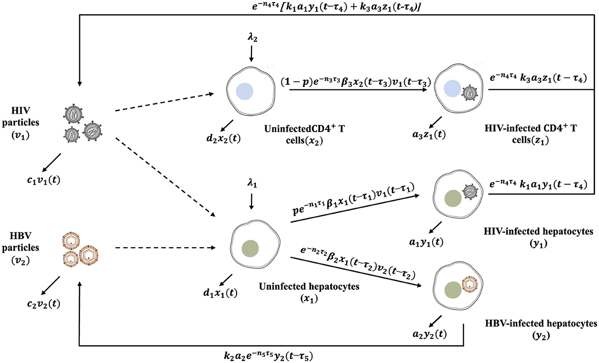
Figure 1. Schematic diagram for HIV/HBV co-infection dynamics within the host.

Based on Hypotheses (H1)-(H8), we formulate an HIV-HBV co-dynamics model with delays as follows:

$\begin{array}{ll}{\dot{x}}_1(t)={\lambda }_1-d_1{x}_1(t)-p{\beta }_1{x}_1(t)v_1(t)-{\beta }_2{x}_1(t)v_2(t),& (1)\end{array}$

$\begin{array}{ll}{\dot{y}}_1(t)=p{e}^{-n_1{\tau }_1}{\beta }_1{x}_1(t-{\tau }_1)v_1(t-{\tau }_1)-a_1{y}_1(t),& (2)\end{array}$

$\begin{array}{ll}{\dot{y}}_2(t)=e^{-n_2{\tau }_2}{\beta }_2{x}_1(t-{\tau }_2)v_2(t-{\tau }_2)-a_2{y}_2(t),& (3)\end{array}$

$\begin{array}{ll}{\dot{x}}_2(t)={\lambda }_2-d_2{x}_2(t)-(1-p){\beta }_3{x}_2(t)v_1(t),& (4)\end{array}$

$\begin{array}{ll}{\dot{z}}_1(t)=(1-p)e^{-n_3{\tau }_3}{\beta }_3{x}_2(t-{\tau }_3)v_1(t-{\tau }_3)-a_3{z}_1(t),& (5)\end{array}$

$\begin{array}{ll}{\dot{v}}_1(t)=e^{-n_4{\tau }_4}\left[k_1{a}_1{y}_1(t-{\tau }_4)+k_3{a}_3{z}_1(t-{\tau }_4)\right]-c_1{v}_1(t),& (6)\end{array}$

$\begin{array}{ll}{\dot{v}}_2(t)=k_2{a}_2{e}^{-n_5{\tau }_5}{y}_2(t-{\tau }_5)-c_2{v}_2(t).& (7)\end{array}$

The model incorporates five distinct time delays:

• The parameters τ₁, τ₂, and τ₃ correspond to the delays associated with the development of HIV-infected hepatocytes, HBV-infected hepatocytes and HIV-infected CD4⁺ T cells, respectively [28, 29]. The expression $e^{-n_i{\tau }_i}$ for i = 1, 2, 3, denotes the likelihood that hepatocytes or CD4⁺ T cells survive during the interval [t − τ_i, t], where n_i > 0.

• The delays τ₄, and τ₅ represent the time required for newly released HIV and HBV to become mature, respectively. Similarly, the term $e^{-n_i{\tau }_i}$ for i = 4, 5 reflects the survival probability of viral particles throughout the corresponding maturation period [t − τ_i, t], assuming n_i > 0.

The initial conditions for model (Equations 1–7) are given as follows:

$\{\begin{array}{l}(x_1,y_1,y_2,x_2,z_1,v_1,v_2)(\theta )=({\varphi }_1,{\varphi }_2,{\varphi }_3,{\varphi }_4,{\varphi }_5,{\varphi }_6,{\varphi }_7)(\theta )\hfill \\ {\varphi }_i(\theta )\ge 0,i=1,2,\cdots ,7,\theta \in [-{\tau }^m,0]\hfill \end{array}$

where ${\tau }^m=max\left\{{\tau }_1,{\tau }_2,\cdots ,{\tau }_5\right\},{\varphi }_i\in C(\left[-{\tau }^m,0\right],{ℝ}_{\ge 0})$, and $C:\left[-{\tau }^m,0\right]\to {ℝ}_{\ge 0}$ is the Banach space of continuous functions. The norm is defined as $\parallel {\varphi }_i\parallel ={sup}_{-{\tau }^m\le \theta \le 0}\left|{\varphi }_i(\theta )\right|$ for ϕ_i ∈ C, and i = 1, 2, ⋯ , 7. The standard theory of functional differential equations shows that, model (Equations 1–7) with initial conditions (Equation 2) has a unique solution [30, 31].

The model's variables and parameters are defined in Table 1.

Table 1

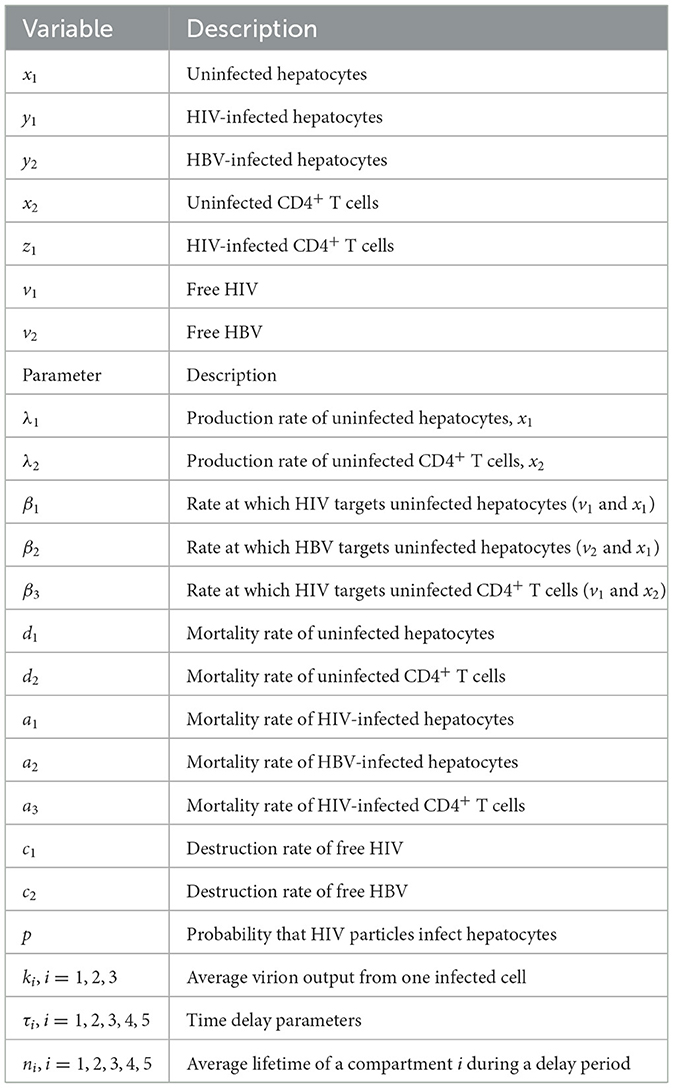
Table 1. Variables and parameters description.

3 Biological feasible domain

Let $F_i=e^{-n_i{\tau }_i}$ for i = 1, 2, ⋯ , 5, σ₁ = min{d₁, a₁, a₂} and σ₂ = min{d₂, a₃}.

Lemma 1. The dynamics (Equations 1–7) with the initial states (Equation 2) admits nonnegative and ultimately bounded solutions.

Proof. Clearly, Equations 1, 4 of model (Equations 1–7) give ẋ_i∣_{xi = 0} = λ_i > 0, which implies that x_i(t) > 0 for i = 1, 2 and all t ≥ 0. Moreover, for t ∈ [0, τ^m] we have

$\begin{array}{l}{y}_1(t)=e^{-a_{1}t}{\varphi }_2(0)+p{\beta }_1{F}_1{\displaystyle {\int }_0^t{e}^{-a_1(t-\theta )}{x}_1(\theta -{\tau }_1)v_1(\theta -{\tau }_1)d\theta ,}\\ y_2(t)=e^{-a_{2}t}{\varphi }_3(0)+{\beta }_2{F}_2{\displaystyle {\int }_0^t{e}^{-a_2(t-\theta )}}{x}_1(\theta -{\tau }_2)v_2(\theta -{\tau }_2)d\theta ,\\ z_1(t)=e^{-a_{3}t}{\varphi }_5(0)+(1-p){\beta }_3{F}_3{\displaystyle {\int }_0^t{e}^{-a_3(t-\theta )}{x}_2(\theta -{\tau }_3)v_1(\theta -{\tau }_3)d\theta ,}\\ v_1(t)=e^{-c_{1}t}{\varphi }_6(0)+F_4{\displaystyle {\int }_0^t{e}^{-c_1(t-\theta )}}[k_1{a}_1{y}_1(\theta -{\tau }_4)+k_3{a}_3{y}_3(\theta -{\tau }_4)]d\theta ,\\ v_2(t)=e^{-c_{2}t}{\varphi }_7(0)+k_2{a}_2{F}_5{\displaystyle {\int }_0^t{e}^{-c_2(t-\theta )}{y}_2(\theta -{\tau }_5)]d\theta 0,}\end{array}$

which gives (x₁, y₁, y₂, x₂, z₁, v₁, v₂)(t) ≥ 0. Hence, by recursive argumentation, we obtain that (x₁, y₁, y₂, x₂, z₁, v₁, v₂)(t) ≥ 0 for any t ≥ 0.

Next we prove the ultimately boundedness of the model's solution (x₁, y₁, y₂, x₂, z₁, v₁, v₂). From Equation 1, we have lim sup_{t → ∞} x₁(t) ≤ Γ₁, where ${\Gamma }_1=\frac{{\lambda }_1}{d_1}$. Concerning, y₁(t) and y₂(t), we define

$\begin{array}{l}{\psi }_1(t)=x_1(t)+\frac{1}{F_1}{y}_1(t+{\tau }_1)+\frac{1}{F_2}{y}_2(t+{\tau }_2).\end{array}$

Then, we get

$\begin{array}{l}{\dot{\psi }}_1(t)={\dot{x}}_1(t)+\frac{1}{F_1}{\dot{y}}_1(t+{\tau }_1)+\frac{1}{F_2}{\dot{y}}_2(t+{\tau }_2)\\ ={\lambda }_1-d_1{x}_1(t)-p{\beta }_1{x}_1(t)v_1(t)-{\beta }_2{x}_1(t)v_2(t)\\ +p{\beta }_1{x}_1(t)v_1(t)-\frac{1}{F_1}{a}_1{y}_1(t+{\tau }_1)+{\beta }_2{x}_1(t)v_2(t)-\frac{1}{F_2}{a}_2{y}_2(t+{\tau }_2)\\ ={\lambda }_1-d_1{x}_1(t)-\frac{1}{F_1}{a}_1{y}_1(t+{\tau }_1)-\frac{1}{F_2}{a}_2{y}_2(t+{\tau }_2)\\ \le {\lambda }_1-{\sigma }_1{\psi }_1(t).\end{array}$

Thus lim sup_{t → ∞} ψ₁(t) ≤ Γ₂, and hence lim sup_{t → ∞} y₁(t) ≤ Γ₂ and lim sup_{t → ∞} y₂(t) ≤ Γ₂, where ${\Gamma }_2=\frac{{\lambda }_1}{{\sigma }_1}$. From Equation 4, we have lim sup_{t → ∞} x₂(t) ≤ Γ₃, where ${\Gamma }_3=\frac{{\lambda }_2}{d_2}$. Define

$\begin{array}{l}{\psi }_2(t)=x_2(t)+\frac{1}{F_3}{z}_1(t+{\tau }_3).\end{array}$

Then, we get

$\begin{array}{l}{\dot{\psi }}_2(t)={\dot{x}}_2(t)+\frac{1}{F_3}{\dot{z}}_1(t+{\tau }_3)\\ ={\lambda }_2-d_2{x}_2(t)-(1-p){\beta }_3{x}_2(t)v_1(t)+(1-p){\beta }_3{x}_2(t)v_1(t)\\ -\frac{a_3}{F_3}{z}_1(t+{\tau }_3)\\ ={\lambda }_2-d_2{x}_2(t)-\frac{a_3}{F_3}{z}_1(t+{\tau }_3)\\ \le {\lambda }_2-{\sigma }_2{\psi }_2(t).\end{array}$

This gives lim sup_{t → ∞} ψ₂(t) ≤ Γ₄, and hence lim sup_{t → ∞} z₁(t) ≤ Γ₄ where ${\Gamma }_4=\frac{{\lambda }_2}{{\sigma }_2}$.

Note that

$\begin{array}{l}{\dot{v}}_1(t)=F_4\left[k_1{a}_1{y}_1(t-{\tau }_4)+k_3{a}_3{z}_1(t-{\tau }_4)\right]-c_1{v}_1(t)\\ \le F_4\left[k_1{a}_1{\Gamma }_2+k_3{a}_3{\Gamma }_4\right]-c_1{v}_1(t)\\ \le k_1{a}_1{\Gamma }_2+k_3{a}_3{\Gamma }_4-c_1{v}_1(t).\end{array}$

Consequently, lim sup_{t → ∞} v₁(t) ≤ Γ₅, where ${\Gamma }_5=\frac{1}{c_1}\left[k_1{a}_1{\Gamma }_2+k_3{a}_3{\Gamma }_4\right]$.

Similarly, we have

$\begin{array}{l}{\dot{v}}_2(t)=F_5{k}_2{a}_2{y}_2(t-{\tau }_5)-c_2{v}_2(t)\le F_5{k}_2{a}_2{\Gamma }_2-c_2{v}_2(t)\le k_2{a}_2{\Gamma }_2-c_2{v}_2(t).\end{array}$

This yields lim sup_{t → ∞} v₂(t) ≤ Γ₆, where ${\Gamma }_6=\frac{k_2{a}_2{\Gamma }_2}{c_2}$.

Based on Lemma 1, one can show

$\begin{array}{l}\Delta =\{\left(x_1,y_1,y_2,x_2,z_1,v_1,v_2\right)\in C_{\ge 0}^7:\Vert x_1\Vert \le {\Gamma }_1,\Vert y_1\Vert \le {\Gamma }_2,\Vert y_2\Vert \\ \le {\Gamma }_2,\Vert x_2\Vert \le {\Gamma }_3,\Vert z_1\Vert \le {\Gamma }_4,\Vert v_1\Vert \le {\Gamma }_5,\Vert v_2\Vert \le {\Gamma }_6\},\end{array}$

is positively invariant w.r.t. system (Equation 1–7).

3.1 Equilibria and thresholds

This section analyzes the existence of equilibria for the proposed model. To compute the basic reproduction number, ${\mathcal{R}}_C$, associated with the HIV-HBV co-infection dynamics, we utilize the next-generation matrix approach as described by [32] (refer to the Appendix for details). The expression obtained for ${\mathcal{R}}_C$:

$\begin{array}{l}{\mathcal{R}}_C=max\left\{{\mathcal{R}}_0,{\mathcal{R}}_1\right\},\end{array}$

where ${\mathcal{R}}_0={\mathcal{R}}_{01}+{\mathcal{R}}_{02},$ and

$\begin{array}{l}{\mathcal{R}}_{01}=\frac{k_{1}p{\beta }_1{\lambda }_1{F}_1{F}_4}{c_1{d}_1},{\mathcal{R}}_{02}=\frac{k_3(1-p){\beta }_3{\lambda }_2{F}_3{F}_4}{c_1{d}_2},\text{and}\\ {\mathcal{R}}_1=\frac{k_2{\beta }_2{\lambda }_1{F}_2{F}_5}{c_2{d}_1}.\end{array}$

Here, ${\mathcal{R}}_0$ represents the basic reproduction number for an HIV infection in isolation, while ${\mathcal{R}}_1$ corresponds to that of HBV infection alone (see Appendix for derivation). Let us define $x_1^0=\frac{{\lambda }_1}{d_1}$ and $x_2^0=\frac{{\lambda }_2}{d_2}$ and let the following two indices be denoted by ${\mathcal{R}}_i>0,$ i = 2, 3 and given by

$\begin{array}{l}{\mathcal{R}}_2=\frac{(1-p)k_2{\beta }_2{k}_3{\beta }_3{\lambda }_2{F}_2{F}_3{F}_5}{k_{1}p{\beta }_1{c}_2{d}_2{F}_1\left(\frac{{\mathcal{R}}_1}{{\mathcal{R}}_{01}}-1\right)},\text{and }{\mathcal{R}}_3=\frac{d_1(1-p){\beta }_3}{p{\beta }_1{d}_2}\left(\frac{{\mathcal{R}}_1-1}{{\mathcal{R}}_2-1}\right).\end{array}$

Therefore, we obtain the following main result regarding the existence of the equilibria of the system (Equations 1–7).

Lemma 2.

• The system (Equation 1–7) admits an infection-free equilibrium denoted by ${\mathcal{E}}_0=(x_1^0,0,0,x_2^0,0,0,0)$.

• If ${\mathcal{R}}_0>1$, then the system admits an HIV-only infection equilibrium denoted by

$\begin{array}{l}\bar{\mathcal{E}}=\left({\bar{x}}_1,{\bar{y}}_1,0,{\bar{x}}_2,{\bar{z}}_1,{\bar{v}}_1,0\right).\end{array}$

• When ${\mathcal{R}}_1>1$, the system admits an HBV-only infection equilibrium denoted by

$\begin{array}{l}\tilde{\mathcal{E}}=\left(\frac{x_1^0}{{\mathcal{R}}_1},0,\frac{c_2{d}_1}{a_2{k}_2{\beta }_2{F}_5}({\mathcal{R}}_1-1),x_2^0,0,0,\frac{d_1}{{\beta }_2}({\mathcal{R}}_1-1)\right).\end{array}$

• If ${\mathcal{R}}_1>{\mathcal{R}}_{01}$, ${\mathcal{R}}_2>1$, and ${\mathcal{R}}_3>1$, the system possesses an HIV and HBV co-infection equilibrium denoted by

$\begin{array}{l}{\mathcal{E}}^{*}=\left(x_1^{*},y_1^{*},y_2^{*},x_2^{*},z_1^{*},v_1^{*},v_2^{*}\right).\end{array}$

Proof. The equilibrium points are normally given when the time-derivatives are all set to zero, so that here we have the following:

$\{\begin{array}{l}0={\lambda }_1-d_1{x}_1-p{\beta }_1{x}_1{v}_1-{\beta }_2{x}_1{v}_2,\hfill \\ 0=p{\beta }_1{F}_1{x}_1{v}_1-a_1{y}_1,\hfill \\ 0={\beta }_2{F}_2{x}_1{v}_2-a_2{y}_2,\hfill \\ 0={\lambda }_2-d_2{x}_2-(1-p){\beta }_3{x}_2{v}_1,\hfill \\ 0=(1-p){\beta }_3{F}_3{x}_2{v}_1-a_3{z}_1,\hfill \\ 0=k_1{a}_1{F}_4{y}_1+k_3{a}_3{F}_4{z}_1-c_1{v}_1,\hfill \\ 0=k_2{a}_2{F}_5{y}_2-c_2{v}_2.\hfill \end{array}$

We have the following cases:

1. If v₁ = v₂ = 0, the model has infection-free equilibrium ${\mathcal{E}}_0=(x_1^0,0,0,x_2^0,0,0,0)$.

2. If v₁ ≠ 0 and v₂ = 0, we obtain

$\begin{array}{l}{y}_2=0,x_1=\frac{{\lambda }_1}{d_1+p{\beta }_1{v}_1},x_2=\frac{{\lambda }_2}{d_2+(1-p){\beta }_3{v}_1},\\ y_1=\frac{p{\beta }_1{\lambda }_1{F}_1{v}_1}{a_1(d_1+p{\beta }_1{v}_1)},z_1=\frac{(1-p){\beta }_3{\lambda }_2{F}_3{v}_1}{a_3(d_2+(1-p){\beta }_3{v}_1)},\end{array}$

and v₁ satisfies the following equation

$\begin{array}{l}\frac{k_{1}p{\beta }_1{\lambda }_1{F}_1{F}_4}{d_1+p{\beta }_1{v}_1}+\frac{k_3(1-p){\beta }_3{\lambda }_2{F}_3{F}_4}{d_2+(1-p){\beta }_3{v}_1}-c_1=0.\end{array}$

Define a function f by

$\begin{array}{l}f(v_1)=\frac{k_{1}p{\beta }_1{\lambda }_1{F}_1{F}_4}{d_1+p{\beta }_1{v}_1}+\frac{k_3(1-p){\beta }_3{\lambda }_2{F}_3{F}_4}{d_2+(1-p){\beta }_3{v}_1}-c_1,\end{array}$

Then we have

$\begin{array}{l}f(0)=\frac{k_{1}p{\beta }_1{\lambda }_1{F}_1{F}_4}{d_1}+\frac{k_3(1-p){\beta }_3{\lambda }_2{F}_3{F}_4}{d_2}-c_1\\ =c_1\left(\frac{k_{1}p{\beta }_1{\lambda }_1{F}_1{F}_4}{c_1{d}_1}+\frac{k_3(1-p){\beta }_3{\lambda }_2{F}_3{F}_4}{c_1{d}_2}-1\right)\\ =c_1({\mathcal{R}}_{01}+{\mathcal{R}}_{02}-1)=c_1({\mathcal{R}}_0-1).\end{array}$

Thus, f(0) > 0 when ${\mathcal{R}}_0>1$. In fact, ${\mathcal{R}}_{01}$ and ${\mathcal{R}}_{02}$ denote, respectively, the total number of newly HIV-infected hepatocytes and HIV-infected CD4⁺ T cells generated from a single HIV-infected hepatocyte and CD4⁺ T cell at the onset of HIV infection. The parameter ${\mathcal{R}}_0$ represents the basic reproductive number for a single HIV infection. We have f(v₁) → −c₁ < 0 whenever v₁ → ∞. Moreover,

$\begin{array}{l}{f}^{\prime }(v_1)=-\left(\frac{k_1{p}^2{\beta }_1^2{\lambda }_1{F}_1{F}_4}{{(d_1+p{\beta }_1{v}_1)}^2}+\frac{k_3{(1-p)}^2{\beta }_3^2{\lambda }_2{F}_3{F}_4}{{(d_2+(1-p){\beta }_3{v}_1)}^2}\right)<0.\end{array}$

Thus, f is strictly decreasing, and hence, if ${\mathcal{R}}_0>1$, there exists a unique ${\bar{v}}_1\in (0,\infty )$ satisfying $f({\bar{v}}_1)=0$. Hence, ${\bar{x}}_1=\frac{{\lambda }_1}{d_1+p{\beta }_1{\bar{v}}_1}>0$, ${\bar{y}}_1=\frac{p{\beta }_1{\lambda }_1{\bar{v}}_1{F}_1}{a_1(d_1+p{\beta }_1{\bar{v}}_1)}>0$, ${\bar{x}}_2=\frac{{\lambda }_2}{d_2+(1-p){\beta }_3{\bar{v}}_1}>0$, and ${\bar{z}}_1=\frac{(1-p){\beta }_3{\lambda }_2{\bar{v}}_1{F}_3}{a_3(d_2+(1-p){\beta }_3{\bar{v}}_1)}>0$, where ${\bar{v}}_1$ satisfies the following quadratic equation:

$\begin{array}{l}-k_{1}p{\beta }_1{\lambda }_1{F}_1{F}_4(d_2+(1-p){\beta }_3{\bar{v}}_1)-k_3(1-p){\beta }_3{\lambda }_2{F}_3{F}_4(d_1)\\ +p{\beta }_1{\bar{v}}_1+c_1(d_1+p{\beta }_1{\bar{v}}_1)(d_2+(1-p){\beta }_3{\bar{v}}_1)=0,\end{array}$

which takes the form

$\begin{array}{ll}a{\bar{v}}_1^2+b{\bar{v}}_1+c=0,& (8)\end{array}$

where

$\begin{array}{l}a=c_{1}p{\beta }_1(1-p){\beta }_3>0,\\ b=c_1(p{\beta }_1{d}_2+(1-p){\beta }_3{d}_1)-p{\beta }_1(1-p){\beta }_3{F}_4(k_1{\lambda }_1{F}_1\\ +k_3{\lambda }_2{F}_3),\\ c=c_1{d}_1{d}_2-k_{1}p{\beta }_1{\lambda }_1{d}_2{F}_1{F}_4-k_3(1-p){\beta }_3{\lambda }_2{d}_1{F}_3{F}_4\\ =c_1{d}_1{d}_2\left(1-\frac{k_{1}p{\beta }_1{\lambda }_1{F}_1{F}_4}{c_1{d}_1}-\frac{k_3(1-p){\beta }_3{\lambda }_2{F}_3{F}_4}{c_1{d}_2}\right)\\ =c_1{d}_1{d}_2\left(1-{ℛ}_0\right).\end{array}$

Clearly, c < 0 if ${\mathcal{R}}_0>1$. Equation 8 has a positive solution

$\begin{array}{l}{\bar{v}}_1=\frac{-b+\sqrt{b^2-4ac}}{2a}>0.\end{array}$

We obtain an HIV-only infection equilibrium

$\begin{array}{l}\bar{\mathcal{E}}=({\bar{x}}_1,{\bar{y}}_1,0,{\bar{x}}_2,{\bar{z}}_1,{\bar{v}}_1,0).\end{array}$

This implies that $\bar{\mathcal{E}}$ exists when ${\mathcal{R}}_0>1$.

3. If v₁ = 0 and v₂ ≠ 0, we obtain an HBV-only infection equilibrium

$\begin{array}{l}\widetilde{ℰ}=\left({\tilde{x}}_1,0,{\tilde{y}}_2,{\tilde{x}}_2,0,0,{\tilde{v}}_2\right)=(\frac{x_1^0}{{ℛ}_1},0,\frac{c_2{d}_1}{a_2{k}_2{\beta }_2{F}_5}({ℛ}_1-1),x_2^0,0,\\ 0,\frac{d_1}{{\beta }_2}({ℛ}_1-1)).\end{array}$

Clearly, $\tilde{\mathcal{E}}$ exists when ${\mathcal{R}}_1>1$.

4. If v₁ ≠ 0 and v₂ ≠ 0, we obtain an HIV and HBV co-infection equilibrium

$\begin{array}{l}{\mathcal{E}}^{*}=(x_1^{*},y_1^{*},y_2^{*},x_2^{*},z_1^{*},v_1^{*},v_2^{*})\end{array}$

where

$\begin{array}{l}{x}_1^{*}=\frac{x_1^0}{{\mathcal{R}}_1},y_1^{*}=\frac{c_2{d}_{2}p{\beta }_1{F}_1}{k_2{\beta }_2(1-p){\beta }_3{a}_1{F}_2{F}_5}({\mathcal{R}}_2-1),\\ y_2^{*}=\frac{c_2{d}_{2}p{\beta }_1}{(1-p){\beta }_2{\beta }_3{a}_2{k}_2{F}_5}({\mathcal{R}}_2-1)({\mathcal{R}}_3-1),\\ x_2^{*}=\frac{k_{1}p{\beta }_1{c}_2{F}_1}{(1-p)k_2{\beta }_2{k}_3{\beta }_3{F}_2{F}_3{F}_5}\left(\frac{{\mathcal{R}}_1}{{\mathcal{R}}_{01}}-1\right),\\ z_1^{*}=\frac{k_{1}p{\beta }_1{c}_2{d}_2{F}_1}{a_3(1-p)k_2{\beta }_2{k}_3{\beta }_3{F}_2{F}_5}\left(\frac{{\mathcal{R}}_1}{{\mathcal{R}}_{01}}-1\right)({\mathcal{R}}_2-1),\\ v_1^{*}=\frac{d_2}{(1-p){\beta }_3}({\mathcal{R}}_2-1),v_2^{*}=\frac{p{\beta }_1{d}_2}{{\beta }_2(1-p){\beta }_3}\\ ({\mathcal{R}}_2-1)({\mathcal{R}}_3-1).\end{array}$

It is evident that ${\mathcal{E}}^{*}$ exists if ${\mathcal{R}}_1>{\mathcal{R}}_{01}$, ${\mathcal{R}}_2>1$, and ${\mathcal{R}}_3>1$. This equilibrium represents the coexistence of HIV and HBV infections.

4 Global stability

The global asymptotic stability of all equilibrium points in the system (Equations 1–7) is investigated using Lyapunov's direct method in this section. The development of Lyapunov functions is based on the approach outlined in [33]. Let $\mathcal{F}$ represent the candidate Lyapunov function, and let Ω′ denote the largest invariant subset of $\Omega =\left\{(x_1,y_1,y_2,x_2,z_1,v_1,v_2):\frac{d\mathcal{F}}{dt}=0\right\}$. Consider the function Φ(X) = X − ln X − 1. Let us denote by (x₁, y₁, y₂, x₂, z₁, v₁, v₂) = (x₁, y₁, y₂, x₂, z₁, v₁, v₂)(t), and $(x_1^{\tau },y_1^{\tau },y_2,x_2^{\tau },z_1^{\tau },v_1^{\tau },v_2^{\tau })=(x_1,y_1,y_2,x_2,z_1,v_1,v_2)(t-\tau )$.

Theorem 1. The infection-free equilibrium ${\mathcal{E}}_0$ is globally asymptotically stable (GAS) when ${\mathcal{R}}_C\le 1$.

Proof. Consider ${\mathcal{F}}_0(x_1,y_1,y_2,x_2,z_1,v_1,v_2)$

$\begin{array}{l}{\mathcal{F}}_0=x_1^0\Phi \left(\frac{x_1}{x_1^0}\right)+\frac{1}{F_1}{y}_1+\frac{1}{F_2}{y}_2+\frac{F_3}{F_1}\frac{k_3}{k_1}{x}_2^0\Phi \left(\frac{x_2}{x_2^0}\right)+\frac{1}{F_1}\frac{k_3}{k_1}{z}_1\\ +\frac{1}{F_1{F}_4{k}_1}{v}_1+\frac{1}{F_2{F}_5{k}_2}{v}_2+p{\beta }_1{\displaystyle {\int }_{t-{\tau }_1}^t}{x}_1(\theta )v_1(\theta )d\theta \\ +{\beta }_2{\displaystyle {\int }_{t-{\tau }_2}^t}{x}_1(\theta )v_2(\theta )d\theta \\ +(1-p){\beta }_3\frac{k_3}{k_1}\frac{F_3}{F_1}{\displaystyle {\int }_{t-{\tau }_3}^t}{x}_2(\theta )v_1(\theta )d\theta \\ +\frac{1}{F_1{k}_1}{\displaystyle {\int }_{t-{\tau }_4}^t}(k_1{a}_1{y}_1(\theta )+k_3{a}_3{z}_1(\theta ))d\theta \\ +\frac{1}{F_2}{a}_2{\displaystyle {\int }_{t-{\tau }_5}^t}{y}_2(\theta )d\theta .\end{array}$

Calculating $\frac{d{\mathcal{F}}_0}{dt}$ along the solution of system (Equations 1–7) as

$\begin{array}{l}\frac{d{\mathcal{F}}_0}{dt}=\left(1-\frac{x_1^0}{x_1}\right){\dot{x}}_1+\frac{1}{F_1}{\dot{y}}_1+\frac{1}{F_2}{\dot{y}}_2+\frac{F_3}{F_1}\frac{k_3}{k_1}\left(1-\frac{x_2^0}{x_2}\right){\dot{x}}_2\\ +\frac{1}{F_1}\frac{k_3}{k_1}{\dot{z}}_1+\frac{1}{k_1{F}_1{F}_4}{\dot{v}}_1+\frac{1}{k_2{F}_2{F}_5}{\dot{v}}_2\\ +p{\beta }_1\left(x_1{v}_1-x_1^{{\tau }_1}{v}_1^{{\tau }_1}\right)+{\beta }_2\left(x_1{v}_2-x_1^{{\tau }_2}{v}_2^{{\tau }_2}\right)\\ +\left(1-p\right){\beta }_3\frac{k_3}{k_1}\frac{F_3}{F_1}\left(x_2{v}_1-x_2^{{\tau }_3}{v}_1^{{\tau }_3}\right)\\ +\frac{1}{k_1{F}_1}\left(k_1{a}_1{y}_1+k_3{a}_3{z}_1-k_1{a}_1{y}_1^{{\tau }_4}-k_3{a}_3{z}_1^{{\tau }_4}\right)\\ +\frac{1}{F_2}{a}_2\left(y_2-y_2^{{\tau }_5}\right).\end{array}$

From Equations 1–7 we obtain

$\begin{array}{l}\frac{d{\mathcal{F}}_0}{dt}=\left(1-\frac{x_1^0}{x_1}\right)\left({\lambda }_1-d_1{x}_1-p{\beta }_1{x}_1{v}_1-{\beta }_2{x}_1{v}_2\right)+p{\beta }_1{x}_1^{{\tau }_1}{v}_1^{{\tau }_1}\\ -\frac{1}{F_1}{a}_1{y}_1+{\beta }_2{x}_1^{{\tau }_2}{v}_2^{{\tau }_2}-\frac{1}{F_2}{a}_2{y}_2+\frac{F_3}{F_1}\frac{k_3}{k_1}\left(1-\frac{x_2^0}{x_2}\right)\\ \left({\lambda }_2-d_2{x}_2-\left(1-p\right){\beta }_3{x}_2{v}_1\right)\\ +\frac{1}{F_1}\frac{k_3}{k_1}\left(\left(1-p\right)F_3{\beta }_3{x}_2^{{\tau }_3}{v}_1^{{\tau }_3}-a_3{z}_1\right)+\frac{1}{k_1{F}_1{F}_4}\\ \left[F_4\left(k_1{a}_1{y}_1^{{\tau }_4}+k_3{a}_3{z}_1^{{\tau }_4}\right)-c_1{v}_1\right]\\ +\frac{1}{k_2{F}_2{F}_5}\left(k_2{a}_2{F}_5{y}_2^{{\tau }_5}-c_2{v}_2\right)\\ +p{\beta }_1\left(x_1{v}_1-x_1^{{\tau }_1}{v}_1^{{\tau }_1}\right)+{\beta }_2\left(x_1{v}_2-x_1^{{\tau }_2}{v}_2^{{\tau }_2}\right)\\ +\left(1-p\right){\beta }_3\frac{k_3}{k_1}\frac{F_3}{F_1}\left(x_2{v}_1-x_2^{{\tau }_3}{v}_1^{{\tau }_3}\right)\\ +\frac{1}{k_1{F}_1}\left(k_1{a}_1{y}_1+k_3{a}_3{z}_1-k_1{a}_1{y}_1^{{\tau }_4}-k_3{a}_3{z}_1^{{\tau }_4}\right)\\ +\frac{1}{F_2}{a}_2\left(y_2-y_2^{{\tau }_5}\right).\end{array}$

Collecting terms as

$\begin{array}{l}\frac{d{\mathcal{F}}_0}{dt}=\left(1-\frac{x_1^0}{x_1}\right)\left({\lambda }_1-d_1{x}_1\right)+p{\beta }_1{x}_1^0{v}_1+{\beta }_2{x}_1^0{v}_2\\ +\frac{F_3{k}_3}{F_1{k}_1}\left(1-\frac{x_2^0}{x_2}\right)\left({\lambda }_2-d_2{x}_2\right)+\frac{F_3{k}_3}{F_1{k}_1}\left(1-p\right){\beta }_3{x}_2^0{v}_1\\ -\frac{c_1}{k_1{F}_1{F}_4}{v}_1-\frac{c_2}{k_2{F}_2{F}_5}{v}_2.\end{array}$

Substituting ${\lambda }_1=d_1{x}_1^0$ and ${\lambda }_2=d_2{x}_2^0$, we obtain

$\begin{array}{l}\frac{d{\mathcal{F}}_0}{dt}=-\frac{d_1}{x_1}{\left(x_1-x_1^0\right)}^2-\frac{F_3{k}_3{d}_2}{F_1{k}_1{x}_2}{\left(x_2-x_2^0\right)}^2\\ +\frac{c_1}{F_1{F}_4{k}_1}\left(F_1{F}_4\frac{p{\beta }_1{k}_1}{c_1}{x}_1^0+F_3{F}_4\frac{\left(1-p\right){\beta }_3{k}_3}{c_1}{x}_2^0-1\right)v_1\\ +\frac{c_2}{F_2{F}_5{k}_2}\left(F_2{F}_5\frac{{\beta }_2{k}_2}{c_2}{x}_1^0-1\right)v_2\\ =-\frac{d_1}{x_1}{\left(x_1-x_1^0\right)}^2-\frac{F_3{k}_3{d}_2}{F_1{k}_1{x}_2}{\left(x_2-x_2^0\right)}^2\\ +\frac{c_1}{F_1{F}_4{k}_1}\left({\mathcal{R}}_0-1\right)v_1+\frac{c_2}{F_2{F}_5{k}_2}\left({\mathcal{R}}_1-1\right)v_2.\end{array}$

Therefore, for all x₁, y₁, y₂, x₂, z₁, v₁, v₂ > 0 we have $\frac{d{\mathcal{F}}_0}{dt}\le 0$ when ${\mathcal{R}}_C\le 1$. Moreover, $\frac{d{\mathcal{F}}_0}{dt}=0$ when $x_1=x_1^0$ , $x_2=x_2^0$, $\left({\mathcal{R}}_0-1\right)v_1=0$, and $\left({\mathcal{R}}_1-1\right)v_2=0$. According to [30], solutions of system (Equation 1–7) asymptotically approach the set ${\Omega }_0^{\prime }$, which consists of elements satisfying $x_1\left(t\right)=x_1^0$, $x_2\left(t\right)=x_2^0$ and

$\begin{array}{ll}\left({\mathcal{R}}_0-1\right)v_1=0,& (9)\end{array}$

$\begin{array}{ll}\left({\mathcal{R}}_1-1\right)v_2=0.& (10)\end{array}$

Let us consider four cases:

• If ${\mathcal{R}}_C<1$ then ${\mathcal{R}}_0<1$ and ${\mathcal{R}}_1<1$ and from Equations 9, 10, we obtain v₁ = v₂ = 0. Since ${\Omega }_0^{\prime }$ is invariant, we obtain ${\dot{v}}_1\left(t\right)={\dot{v}}_2\left(t\right)=0$. From Equations 6, 7, we have

$\begin{array}{ll}0={\dot{v}}_1=F_4{k}_1{a}_1{y}_1^{{\tau }_4}+F_4{k}_3{a}_3{z}_1^{{\tau }_4}\Rightarrow y_1\left(t\right)=z_1\left(t\right)=0,\forall t\ge 0,& (11)\end{array}$

and

$\begin{array}{ll}0={\dot{v}}_2=F_5{k}_2{a}_2{y}_2^{{\tau }_5}\Rightarrow y_2\left(t\right)=0,\forall t\ge 0.& (12)\end{array}$

Hence, ${\Omega }_0^{\prime }=\left\{{\mathcal{E}}_0\right\}.$

• If ${\mathcal{R}}_0={\mathcal{R}}_1=1$, we have $x_1=x_1^0$, $x_2=x_2^0$ then ẋ₁(t) = ẋ₂(t) = 0. From Equations 1, 4, we have

$\begin{array}{ll}{\lambda }_2-d_2{x}_2^0-\left(1-p\right){\beta }_3{x}_2^0{v}_1=0\Rightarrow v_1\left(t\right)=0,\forall t\ge 0.& (13)\end{array}$

$\begin{array}{ll}{\lambda }_1-d_1{x}_1^0-p{\beta }_1{x}_1^0{v}_1-{\beta }_2{x}_1^0{v}_2=0\Rightarrow v_2\left(t\right)=0,\forall t\ge 0,& (14)\end{array}$

Equations 11, 12 imply y₁(t) = z₁(t) = y₂(t) = 0, ∀t ≥ 0. Hence, ${\Omega }_0^{\prime }=\left\{{\mathcal{E}}_0\right\}$.

• If ${\mathcal{R}}_0<1$ and ${\mathcal{R}}_1=1$ then v₁ = 0 and thus Equation 14 gives v₂(t) = 0, ∀t ≥ 0 and from Equations 11, 12, we obtain y₁ = z₁ = y₂ = 0. Hence, ${\bar{\Omega }}^{\prime }=\left\{{\mathcal{E}}_0\right\}$.

• Similarly, if ${\mathcal{R}}_0=1$ and ${\mathcal{R}}_1<1$ then v₂ = 0 and thus Equation 13 provides v₁(t) = 0, ∀t ≥ 0. From Equations 11, 12, we obtain y₁ = z₁ = y₂ = 0. Hence, ${\Omega }_0^{\prime }=\left\{{\mathcal{E}}_0\right\}$.

Lyapunov-LaSalle asymptotic stability theorem [34–36] reveals that ${\mathcal{E}}_0=\left(x_1^0,0,0,x_2^0,0,0,0\right)$ is GAS when ${\mathcal{R}}_C\le 1$.

Theorem 2. If the HIV-only infection equilibrium $\bar{\mathcal{E}}$ exists (${\mathcal{R}}_0>1$) then it is GAS under the condition ${\mathcal{R}}_1\le 1+\frac{p{\beta }_1{\bar{v}}_1}{d_1}$.

Proof. Define a function $\bar{\mathcal{F}}\left(x_1,y_1,y_2,x_2,z_1,v_1,v_2\right)$

$\begin{array}{l}\bar{\mathcal{F}}={\bar{x}}_1\Phi \left(\frac{x_1}{{\bar{x}}_1}\right)+\frac{1}{F_1}{\bar{y}}_1\Phi \left(\frac{y_1}{{\bar{y}}_1}\right)+\frac{1}{F_2}{y}_2+\frac{F_3}{F_1}\frac{k_3}{k_1}{\bar{x}}_2\Phi \left(\frac{x_2}{{\bar{x}}_2}\right)\\ +\frac{1}{F_1}\frac{k_3}{k_1}{\bar{z}}_1\Phi \left(\frac{z_1}{{\bar{z}}_1}\right)+\frac{1}{k_1{F}_1{F}_4}{\bar{v}}_1\Phi \left(\frac{v_1}{{\bar{v}}_1}\right)+\frac{1}{k_2{F}_2{F}_5}{v}_2+p{\beta }_1{\bar{x}}_1{\bar{v}}_1{\displaystyle {\int }_{t-{\tau }_1}^t}\Phi \left(\frac{x_1(\theta )v_1(\theta )}{{\bar{x}}_1{\bar{v}}_1}\right)d\theta \\ +{\beta }_2{\displaystyle {\int }_{t-{\tau }_2}^t}{x}_1(\theta )v_2(\theta )d\theta +\left(1-p\right){\beta }_3\frac{k_3}{k_1}\frac{F_3}{F_1}{\bar{x}}_2{\bar{v}}_1{\displaystyle {\int }_{t-{\tau }_3}^t}\Phi \left(\frac{x_2(\theta )v_1(\theta )}{{\bar{x}}_2{\bar{v}}_1}\right)d\theta \\ +\frac{1}{k_1{F}_1}{\displaystyle {\int }_{t-{\tau }_4}^t}\left(k_1{a}_1{\bar{y}}_1\Phi \left(\frac{y_1(\theta )}{{\bar{y}}_1}\right)+k_3{a}_3{\bar{z}}_1\Phi \left(\frac{z_1(\theta )}{{\bar{z}}_1}\right)\right)d\theta +\frac{1}{F_2}{a}_2{\displaystyle {\int }_{t-{\tau }_5}^t}{y}_2(\theta )d\theta .\end{array}$

We calculate $\frac{d\bar{\mathcal{F}}}{dt}$ as follows:

$\begin{array}{l}\frac{d\bar{\mathcal{F}}}{dt}=\left(1-\frac{{\bar{x}}_1}{x_1}\right)\left({\lambda }_1-d_1{x}_1-p{\beta }_1{x}_1{v}_1-{\beta }_2{x}_1{v}_2\right)+\frac{1}{F_1}\left(1-\frac{{\bar{y}}_1}{y_1}\right)\left(p{\beta }_1{F}_1{x}_1^{{\tau }_1}{v}_1^{{\tau }_1}-a_1{y}_1\right)\\ +\frac{1}{F_2}\left(F_2{\beta }_2{x}_1^{{\tau }_2}{v}_2^{{\tau }_2}-a_2{y}_2\right)+\frac{F_3}{F_1}\frac{k_3}{k_1}\left(1-\frac{{\bar{x}}_2}{x_2}\right)\left({\lambda }_2-d_2{x}_2-\left(1-p\right){\beta }_3{x}_2{v}_1\right)\\ +\frac{1}{F_1}\frac{k_3}{k_1}\left(1-\frac{{\bar{z}}_1}{z_1}\right)\left(\left(1-p\right){\beta }_3{F}_3{x}_2^{{\tau }_3}{v}_1^{{\tau }_3}-a_3{z}_1\right)+\frac{1}{k_1{F}_1{F}_4}\left(1-\frac{{\bar{v}}_1}{v_1}\right)\left(F_4{k}_1{a}_1{y}_1^{{\tau }_4}+F_4{k}_3{a}_3{z}_1^{{\tau }_4}-c_1{v}_1\right)\\ +\frac{1}{k_2{F}_2{F}_5}\left(F_5{k}_2{a}_2{y}_2^{{\tau }_5}-c_2{v}_2\right)+p{\beta }_1{\bar{x}}_1{\bar{v}}_1\left(\frac{x_1{v}_1}{{\bar{x}}_1{\bar{v}}_1}-\frac{x_1^{{\tau }_1}{v}_1^{{\tau }_1}}{{\bar{x}}_1{\bar{v}}_1}+ln\left(\frac{x_1^{{\tau }_1}{v}_1^{{\tau }_1}}{x_1{v}_1}\right)\right)\\ +{\beta }_2\left(x_1{v}_2-x_1^{{\tau }_2}{v}_2^{{\tau }_2}\right)+\left(1-p\right){\beta }_3\frac{k_3}{k_1}\frac{F_3}{F_1}{\bar{x}}_2{\bar{v}}_1\left(\frac{x_2{v}_1}{{\bar{x}}_2{\bar{v}}_1}-\frac{x_2^{{\tau }_3}{v}_1^{{\tau }_3}}{{\bar{x}}_2{\bar{v}}_1}+ln\left(\frac{x_2^{{\tau }_3}{v}_1^{{\tau }_3}}{x_2{v}_1}\right)\right)\\ +\frac{1}{k_1{F}_1}\left[k_1{a}_1{\bar{y}}_1\left(\frac{y_1}{{\bar{y}}_1}-\frac{y_1^{{\tau }_4}}{{\bar{y}}_1}+ln\left(\frac{y_1^{{\tau }_4}}{y_1}\right)\right)+k_3{a}_3{\bar{z}}_1\left(\frac{z_1}{{\bar{z}}_1}-\frac{z_1^{{\tau }_4}}{{\bar{z}}_1}+ln\left(\frac{z_1^{{\tau }_4}}{z_1}\right)\right)\right]+\frac{1}{F_2}{a}_2\left(y_2-y_2^{{\tau }_5}\right).\end{array}$

Collecting terms, we get

$\begin{array}{l}\frac{d\bar{\mathcal{F}}}{dt}=\left(1-\frac{{\bar{x}}_1}{x_1}\right)\left({\lambda }_1-d_1{x}_1\right)+p{\beta }_1{\bar{x}}_1{v}_1+{\beta }_2{\bar{x}}_1{v}_2-p{\beta }_1\frac{{\bar{y}}_1}{y_1}{x}_1^{{\tau }_1}{v}_1^{{\tau }_1}+\frac{a_1}{F_1}{\bar{y}}_1\\ +\frac{F_3{k}_3}{F_1{k}_1}\left(1-\frac{{\bar{x}}_2}{x_2}\right)\left({\lambda }_2-d_2{x}_2\right)+\frac{F_3{k}_3}{F_1{k}_1}\left(1-p\right){\beta }_3{\bar{x}}_2{v}_1-\frac{F_3{k}_3}{F_1{k}_1}\left(1-p\right){\beta }_3\frac{{\bar{z}}_1}{z_1}{x}_2^{{\tau }_3}{v}_1^{{\tau }_3}\\ +\frac{a_3{k}_3}{F_1{k}_1}{\bar{z}}_1-\frac{a_1}{F_1}\frac{{\bar{v}}_1}{v_1}{y}_1^{{\tau }_4}-\frac{a_3{k}_3}{F_1{k}_1}\frac{{\bar{v}}_1}{v_1}{z}_1^{{\tau }_4}+\frac{c_1}{k_1{F}_1{F}_4}{\bar{v}}_1-\frac{c_1}{k_1{F}_1{F}_4}{v}_1-\frac{c_2}{k_2{F}_2{F}_5}{v}_2\\ +p{\beta }_1{\bar{x}}_1{\bar{v}}_{1}ln\left(\frac{x_1^{{\tau }_1}{v}_1^{{\tau }_1}}{x_1{v}_1}\right)+\frac{F_3{k}_3}{F_1{k}_1}\left(1-p\right){\beta }_3{\bar{x}}_2{\bar{v}}_{1}ln\left(\frac{x_2^{{\tau }_3}{v}_1^{{\tau }_3}}{x_2{v}_1}\right)+\frac{a_1}{F_1}{\bar{y}}_{1}ln\left(\frac{y_1^{{\tau }_4}}{y_1}\right)+\frac{k_3{a}_3}{k_1{F}_1}{\bar{z}}_{1}ln\left(\frac{z_1^{{\tau }_4}}{z_1}\right).\end{array}$

By using the equilibrium conditions

$\begin{array}{l}{\lambda }_1=d_1{\bar{x}}_1+p{\beta }_1{\bar{x}}_1{\bar{v}}_1,{\lambda }_2=d_2{\bar{x}}_2+\left(1-p\right){\beta }_3{\bar{x}}_2{\bar{v}}_1,F_4{k}_1{a}_1{\bar{y}}_1+F_4{k}_3{a}_3{\bar{z}}_1=c_1{\bar{v}}_1,\\ p{F}_1{\beta }_1{\bar{x}}_1{\bar{v}}_1=a_1{\bar{y}}_1,\left(1-p\right)F_3{\beta }_3{\bar{x}}_2{\bar{v}}_1=a_3{\bar{z}}_1,\end{array}$

we obtain

$\begin{array}{l}\frac{d\bar{\mathcal{F}}}{dt}=\left(1-\frac{{\bar{x}}_1}{x_1}\right)\left(d_1{\bar{x}}_1-d_1{x}_1\right)+p{\beta }_1{\bar{x}}_1{\bar{v}}_1\left(1-\frac{{\bar{x}}_1}{x_1}\right)+{\beta }_2{\bar{x}}_1{v}_2-p{\beta }_1\frac{{\bar{y}}_1}{y_1}{x}_1^{{\tau }_1}{v}_1^{{\tau }_1}+p{\beta }_1{\bar{x}}_1{\bar{v}}_1\\ +\frac{F_3{k}_3}{F_1{k}_1}\left(1-\frac{{\bar{x}}_2}{x_2}\right)\left(d_2{\bar{x}}_2-d_2{x}_2\right)+\frac{F_3{k}_3}{F_1{k}_1}\left(1-p\right){\beta }_3{\bar{x}}_2{\bar{v}}_1\left(1-\frac{{\bar{x}}_2}{x_2}\right)\\ -\frac{F_3{k}_3}{F_1{k}_1}\left(1-p\right){\beta }_3\frac{{\bar{z}}_1}{z_1}{x}_2^{{\tau }_3}{v}_1^{{\tau }_3}+\frac{F_3{k}_3}{F_1{k}_1}\left(1-p\right){\beta }_3{\bar{x}}_2{\bar{v}}_1-p{\beta }_1{\bar{x}}_1{\bar{v}}_1\frac{{\bar{v}}_1}{v_1}\frac{y_1^{{\tau }_4}}{{\bar{y}}_1}-\frac{F_3{k}_3}{F_1{k}_1}\left(1-p\right){\beta }_3{\bar{x}}_2{\bar{v}}_1\frac{{\bar{v}}_1}{v_1}\frac{z_1^{{\tau }_4}}{{\bar{z}}_1}\\ +p{\beta }_1{\bar{x}}_1{\bar{v}}_1+\frac{F_3{k}_3}{F_1{k}_1}\left(1-p\right){\beta }_3{\bar{x}}_2{\bar{v}}_1-\frac{c_2{v}_2}{k_2{F}_2{F}_5}+p{\beta }_1{\bar{x}}_1{\bar{v}}_{1}ln\left(\frac{x_1^{{\tau }_1}{v}_1^{{\tau }_1}}{x_1{v}_1}\right)\\ +\frac{F_3{k}_3}{F_1{k}_1}\left(1-p\right){\beta }_3{\bar{x}}_2{\bar{v}}_{1}ln\left(\frac{x_2^{{\tau }_3}{v}_1^{{\tau }_3}}{x_2{v}_1}\right)+p{\beta }_1{\bar{x}}_1{\bar{v}}_{1}ln\left(\frac{y_1^{{\tau }_4}}{y_1}\right)+\frac{F_3{k}_3}{F_1{k}_1}\left(1-p\right){\beta }_3{\bar{x}}_2{\bar{v}}_{1}ln\left(\frac{z_1^{{\tau }_4}}{z_1}\right).\end{array}$

Then

$\begin{array}{l}\frac{d\bar{\mathcal{F}}}{dt}=-d_1\frac{{\left({\bar{x}}_1-x_1\right)}^2}{x_1}-\frac{d_2{F}_3{k}_3}{F_1{k}_1}\frac{{\left({\bar{x}}_2-x_2\right)}^2}{x_2}+\frac{1}{F_2{F}_5}\left(F_2{F}_5{\beta }_2{\bar{x}}_1-\frac{c_2}{k_2}\right)v_2\\ +p{\beta }_1{\bar{x}}_1{\bar{v}}_1\left(3-\frac{{\bar{x}}_1}{x_1}-\frac{x_1^{{\tau }_1}{v}_1^{{\tau }_1}{\bar{y}}_1}{{\bar{x}}_1{\bar{v}}_1{y}_1}-\frac{y_1^{{\tau }_4}{\bar{v}}_1}{{\bar{y}}_1{v}_1}+ln\left(\frac{y_1^{{\tau }_4}}{y_1}\right)+ln\left(\frac{x_1^{{\tau }_1}{v}_1^{{\tau }_1}}{x_1{v}_1}\right)\right)\\ +\frac{F_3{k}_3}{F_1{k}_1}\left(1-p\right){\beta }_3{\bar{x}}_2{\bar{v}}_1\left(3-\frac{{\bar{x}}_2}{x_2}-\frac{x_2^{{\tau }_3}{v}_1^{{\tau }_3}{\bar{z}}_1}{{\bar{x}}_2{\bar{v}}_1{z}_1}-\frac{z_1^{{\tau }_4}{\bar{v}}_1}{{\bar{z}}_1{v}_1}+ln\left(\frac{x_2^{{\tau }_3}{v}_1^{{\tau }_3}}{x_2{v}_1}\right)+ln\left(\frac{z_1^{{\tau }_4}}{z_1}\right)\right).\end{array}$

Using the following equalities:

$\begin{array}{l}ln\left(\frac{y_1^{{\tau }_4}}{y_1}\right)+ln\left(\frac{x_1^{{\tau }_1}{v}_1^{{\tau }_1}}{x_1{v}_1}\right)=ln\left(\frac{{\bar{x}}_1}{x_1}\right)+ln\left(\frac{x_1^{{\tau }_1}{v}_1^{{\tau }_1}{\bar{y}}_1}{{\bar{x}}_1{\bar{v}}_1{y}_1}\right)+ln\left(\frac{y_1^{{\tau }_4}{\bar{v}}_1}{{\bar{y}}_1{v}_1}\right),\\ ln\left(\frac{x_2^{{\tau }_3}{v}_1^{{\tau }_3}}{x_2{v}_1}\right)+ln\left(\frac{z_1^{{\tau }_4}}{z_1}\right)=ln\left(\frac{{\bar{x}}_2}{x_2}\right)+ln\left(\frac{x_2^{{\tau }_3}{v}_1^{{\tau }_3}{\bar{z}}_1}{{\bar{x}}_2{\bar{v}}_1{z}_1}\right)+ln\left(\frac{z_1^{{\tau }_4}{\bar{v}}_1}{{\bar{z}}_1{v}_1}\right),\end{array}$

we obtain

$\begin{array}{l}\frac{d\bar{\mathcal{F}}}{dt}=-d_1\frac{{\left({\bar{x}}_1-x_1\right)}^2}{x_1}-\frac{d_2{F}_3{k}_3}{F_1{k}_1}\frac{{\left({\bar{x}}_2-x_2\right)}^2}{x_2}+\frac{1}{F_2{F}_5}\left(F_2{F}_5{\beta }_2{\bar{x}}_1-\frac{c_2}{k_2}\right)v_2\\ -p{\beta }_1{\bar{x}}_1{\bar{v}}_1\left[\Phi \left(\frac{{\bar{x}}_1}{x_1}\right)+\Phi \left(\frac{x_1^{{\tau }_1}{v}_1^{{\tau }_1}{\bar{y}}_1}{{\bar{x}}_1{\bar{v}}_1{y}_1}\right)+\Phi \left(\frac{y_1^{{\tau }_4}{\bar{v}}_1}{{\bar{y}}_1{v}_1}\right)\right]\\ -\frac{F_3{k}_3}{F_1{k}_1}\left(1-p\right){\beta }_3{\bar{x}}_2{\bar{v}}_1\left[\Phi \left(\frac{{\bar{x}}_2}{x_2}\right)+\Phi \left(\frac{x_2^{{\tau }_3}{v}_1^{{\tau }_3}{\bar{z}}_1}{{\bar{x}}_2{\bar{v}}_1{z}_1}\right)+\Phi \left(\frac{z_1^{{\tau }_4}{\bar{v}}_1}{{\bar{z}}_1{v}_1}\right)\right].\end{array}$

We have

$\begin{array}{l}{F}_2{F}_5{\beta }_2{\bar{x}}_1-\frac{c_2}{k_2}=\frac{F_2{F}_5{\beta }_2{\lambda }_1}{d_1+p{\beta }_1{\bar{v}}_1}-\frac{c_2}{k_2}=\frac{F_2{F}_5{\beta }_2{k}_2{\lambda }_1-c_2{d}_1-c_{2}p{\beta }_1{\bar{v}}_1}{k_2\left(d_1+p{\beta }_1{\bar{v}}_1\right)}=\frac{c_2{d}_1\left({\mathcal{R}}_1-1\right)}{k_2\left(d_1+p{\beta }_1{\bar{v}}_1\right)}-\frac{c_{2}p{\beta }_1{\bar{v}}_1}{k_2\left(d_1+p{\beta }_1{\bar{v}}_1\right)}.\end{array}$

Therefore,

$\begin{array}{l}\frac{d\bar{\mathcal{F}}}{dt}=-d_1\frac{{\left({\bar{x}}_1-x_1\right)}^2}{x_1}-\frac{d_2{F}_3{k}_3}{F_1{k}_1}\frac{{\left({\bar{x}}_2-x_2\right)}^2}{x_2}+\frac{c_2{d}_1}{F_2{F}_5{k}_2\left(d_1+p{\beta }_1{\bar{v}}_1\right)}\left({\mathcal{R}}_1-1-\frac{p{\beta }_1{\bar{v}}_1}{d_1}\right)v_2\\ -p{\beta }_1{\bar{x}}_1{\bar{v}}_1\left[\Phi \left(\frac{{\bar{x}}_1}{x_1}\right)+\Phi \left(\frac{x_1^{{\tau }_1}{v}_1^{{\tau }_1}{\bar{y}}_1}{{\bar{x}}_1{\bar{v}}_1{y}_1}\right)+\Phi \left(\frac{y_1^{{\tau }_4}{\bar{v}}_1}{{\bar{y}}_1{v}_1}\right)\right]\\ -\frac{F_3{k}_3}{F_1{k}_1}\left(1-p\right){\beta }_3{\bar{x}}_2{\bar{v}}_1\left[\Phi \left(\frac{{\bar{x}}_2}{x_2}\right)+\Phi \left(\frac{x_2^{{\tau }_3}{v}_1^{{\tau }_3}{\bar{z}}_1}{{\bar{x}}_2{\bar{v}}_1{z}_1}\right)+\Phi \left(\frac{z_1^{{\tau }_4}{\bar{v}}_1}{{\bar{z}}_1{v}_1}\right)\right].\end{array}$

It follows that $\frac{d\bar{\mathcal{F}}}{dt}\le 0$ when ${\mathcal{R}}_1\le 1+\frac{p{\beta }_1{\bar{v}}_1}{d_1}$. Moreover, $\frac{d\bar{\mathcal{F}}}{dt}=0$ if $\left(x_1,y_1,x_2,z_1,v_1\right)=\left({\bar{x}}_1,{\bar{y}}_1,{\bar{x}}_2,{\bar{z}}_1,{\bar{v}}_1\right)$ and

$\begin{array}{l}\left({\mathcal{R}}_1-1-\frac{p{\beta }_1{\bar{v}}_1}{d_1}\right)v_2=0.\end{array}$

We have two cases:

• ${\mathcal{R}}_1<1+\frac{p{\beta }_1{\bar{v}}_1}{d_1}$. Then v₂ = 0, and hence ${\dot{v}}_2=0$ and from Equation 7 we have $0={\dot{v}}_2=F_5{k}_2{a}_2{y}_2^{{\tau }_5}=0$ and thus y₂(t) = 0, ∀t ≥ 0. Hence, ${\bar{\Omega }}^{\prime }=\left\{\bar{\mathcal{E}}\right\}$.

• ${\mathcal{R}}_1=1+\frac{p{\beta }_1{\bar{v}}_1}{d_1}$. From Equation 1 we have $0={\dot{x}}_1={\lambda }_1-d_1{\bar{x}}_1-p{\beta }_1{\bar{x}}_1{\bar{v}}_1-{\beta }_2{\bar{x}}_1{v}_2$, hence v₂(t) = 0, and from Equation 7 we obtain y₂(t) = 0 for any t. Hence, ${\bar{\Omega }}^{\prime }=\left\{\bar{\mathcal{E}}\right\}$.

Lyapunov-LaSalle asymptotic stability theorem indicates that $\bar{\mathcal{E}}$ is GAS when ${\mathcal{R}}_0>1$ and ${\mathcal{R}}_1\le 1$.

Theorem 3. If the HBV-only infection equilibrium $\tilde{\mathcal{E}}$ exists (if ${\mathcal{R}}_1>1$) then it is GAS under the condition $\frac{{\mathcal{R}}_{01}}{{\mathcal{R}}_1}+{\mathcal{R}}_{02}\le 1$.

Proof. Consider $\tilde{\mathcal{F}}\left(x_1,y_1,y_2,x_2,z_1,v_1,v_2\right)$

$\begin{array}{l}\tilde{\mathcal{F}}={\tilde{x}}_1\Phi \left(\frac{x_1}{{\tilde{x}}_1}\right)+\frac{1}{F_1}{y}_1+\frac{1}{F_2}{\tilde{y}}_2\Phi \left(\frac{y_2}{{\tilde{y}}_2}\right)+\frac{F_3}{F_1}\frac{k_3}{k_1}{\tilde{x}}_2\Phi \left(\frac{x_2}{{\tilde{x}}_2}\right)+\frac{1}{F_1}\frac{k_3}{k_1}{z}_1+\frac{1}{k_1{F}_1{F}_4}{v}_1+\frac{1}{k_2{F}_2{F}_5}{\tilde{v}}_2\Phi \left(\frac{v_2}{{\tilde{v}}_2}\right)\\ +p{\beta }_1{\displaystyle {\int }_{t-{\tau }_1}^t}{x}_1(\theta )v_1(\theta )d\theta +{\beta }_2{\tilde{x}}_1{\tilde{v}}_2{\displaystyle {\int }_{t-{\tau }_2}^t}\Phi \left(\frac{x_1(\theta )v_2(\theta )}{{\tilde{x}}_1{\tilde{v}}_2}\right)d\theta +\frac{F_3}{F_1}\frac{k_3}{k_1}\left(1-p\right){\beta }_3{\displaystyle {\int }_{t-{\tau }_3}^t}{x}_2(\theta )v_1(\theta )d\theta \\ +\frac{1}{k_1{F}_1}{\displaystyle {\int }_{t-{\tau }_4}^t}\left(k_1{a}_1{y}_1(\theta )+k_3{a}_3{z}_1(\theta )\right)d\theta +\frac{1}{F_2}{a}_2{\tilde{y}}_2{\displaystyle {\int }_{t-{\tau }_5}^t}\Phi \left(\frac{y_2(\theta )}{{\tilde{y}}_2}\right)d\theta .\end{array}$

We calculate $\frac{d\tilde{\mathcal{F}}}{dt}$ as:

$\begin{array}{l}\frac{d\tilde{\mathcal{F}}}{dt}=\left(1-\frac{{\tilde{x}}_1}{x_1}\right)\left({\lambda }_1-d_1{x}_1-p{\beta }_1{x}_1{v}_1-{\beta }_2{x}_1{v}_2\right)+\frac{1}{F_1}\left(p{F}_1{\beta }_1{x}_1^{{\tau }_1}{v}_1^{{\tau }_1}-a_1{y}_1\right)\\ +\frac{1}{F_2}\left(1-\frac{{\tilde{y}}_2}{y_2}\right)\left(F_2{\beta }_2{x}_1^{{\tau }_2}{v}_2^{{\tau }_2}-a_2{y}_2\right)+\frac{F_3}{F_1}\frac{k_3}{k_1}\left(1-\frac{{\tilde{x}}_2}{x_2}\right)\left({\lambda }_2-d_2{x}_2-\left(1-p\right){\beta }_3{x}_2{v}_1\right)\\ +\frac{1}{F_1}\frac{k_3}{k_1}\left(\left(1-p\right)F_3{\beta }_3{x}_2^{{\tau }_3}{v}_1^{{\tau }_3}-a_3{z}_1\right)+\frac{1}{k_1{F}_1{F}_4}\left[F_4\left(k_1{a}_1{y}_1^{{\tau }_4}+k_3{a}_3{z}_1^{{\tau }_4}\right)-c_1{v}_1\right]\\ +\frac{1}{k_2{F}_2{F}_5}\left(1-\frac{{\tilde{v}}_2}{v_2}\right)\left(k_2{a}_2{F}_5{y}_2^{{\tau }_5}-c_2{v}_2\right)+p{\beta }_1\left(x_1{v}_1-x_1^{{\tau }_1}{v}_1^{{\tau }_1}\right)\\ +{\beta }_2{\tilde{x}}_1{\tilde{v}}_2\left(\frac{x_1{v}_2}{{\tilde{x}}_1{\tilde{v}}_2}-\frac{x_1^{{\tau }_2}{v}_2^{{\tau }_2}}{{\tilde{x}}_1{\tilde{v}}_2}+ln\left(\frac{x_1^{{\tau }_2}{v}_2^{{\tau }_2}}{x_1{v}_2}\right)\right)+\frac{F_3}{F_1}\frac{k_3}{k_1}\left(1-p\right){\beta }_3\left(x_2{v}_1-x_2^{{\tau }_3}{v}_1^{{\tau }_3}\right)\\ +\frac{1}{k_1{F}_1}\left[k_1{a}_1\left(y_1-y_1^{{\tau }_4}\right)+k_3{a}_3\left(z_1-z_1^{{\tau }_4}\right)\right]+\frac{1}{F_2}{a}_2{\tilde{y}}_2\left(\frac{y_2}{{\tilde{y}}_2}-\frac{y_2^{{\tau }_5}}{{\tilde{y}}_2}+ln\left(\frac{y_2^{{\tau }_5}}{y_2}\right)\right).\end{array}$

Collecting terms as:

$\begin{array}{l}\frac{d\tilde{\mathcal{F}}}{dt}=\left(1-\frac{{\tilde{x}}_1}{x_1}\right)\left({\lambda }_1-d_1{x}_1\right)+p{\beta }_1{\tilde{x}}_1{v}_1+{\beta }_2{\tilde{x}}_1{v}_2-{\beta }_2{x}_1^{{\tau }_2}{v}_2^{{\tau }_2}\frac{{\tilde{y}}_2}{y_2}+\frac{a_2}{F_2}{\tilde{y}}_2+\frac{F_3{k}_3}{F_1{k}_1}\left(1-\frac{{\tilde{x}}_2}{x_2}\right)\left({\lambda }_2-d_2{x}_2\right)\\ +\frac{F_3{k}_3}{F_1{k}_1}\left(1-p\right){\beta }_3{\tilde{x}}_2{v}_1-\frac{c_1}{k_1{F}_1{F}_4}{v}_1-\frac{c_2}{k_2{F}_2{F}_5}{v}_2-\frac{a_2}{F_2}{y}_2^{{\tau }_5}\frac{{\tilde{v}}_2}{v_2}+\frac{c_2}{k_2{F}_2{F}_5}{\tilde{v}}_2+{\beta }_2{\tilde{x}}_1{\tilde{v}}_{2}ln\left(\frac{x_1^{{\tau }_2}{v}_2^{{\tau }_2}}{x_1{v}_2}\right)\\ +\frac{a_2}{F_2}{\tilde{y}}_{2}ln\left(\frac{y_2^{{\tau }_5}}{y_2}\right).\end{array}$

By using the conditions of $\tilde{\mathcal{E}},$

$\begin{array}{l}{\lambda }_1=d_1{\tilde{x}}_1+{\beta }_2{\tilde{x}}_1{\tilde{v}}_2,F_2{\beta }_2{\tilde{x}}_1{\tilde{v}}_2=a_2{\tilde{y}}_2,{\lambda }_2=d_2{\tilde{x}}_2,F_5{k}_2{a}_2{\tilde{y}}_2=F_2{F}_5{k}_2{\beta }_2{\tilde{x}}_1{\tilde{v}}_2=c_2{\tilde{v}}_2,\end{array}$

we obtain

$\begin{array}{l}\frac{d\tilde{\mathcal{F}}}{dt}=-d_1\frac{{\left({\tilde{x}}_1-x_1\right)}^2}{x_1}-\frac{d_2{F}_3{k}_3}{F_1{k}_1}\frac{{\left({\tilde{x}}_2-x_2\right)}^2}{x_2}+\frac{1}{F_1{F}_4}\left(F_1{F}_{4}p{\beta }_1{\tilde{x}}_1+F_3{F}_4\frac{k_3}{k_1}\left(1-p\right){\beta }_3{\tilde{x}}_2-\frac{c_1}{k_1}\right)v_1\\ +{\beta }_2{\tilde{x}}_1{\tilde{v}}_2\left(3-\frac{{\tilde{x}}_1}{x_1}-\frac{y_2^{{\tau }_5}{\tilde{v}}_2}{{\tilde{y}}_2{v}_2}-\frac{x_1^{{\tau }_2}{v}_2^{{\tau }_2}{\tilde{y}}_2}{{\tilde{x}}_1{\tilde{v}}_2{y}_2}+ln\left(\frac{y_2^{{\tau }_5}}{y_2}\right)+ln\left(\frac{x_1^{{\tau }_2}{v}_2^{{\tau }_2}}{x_1{v}_2}\right)\right).\end{array}$

Applying the following equality:

$\begin{array}{l}ln\left(\frac{y_2^{{\tau }_5}}{y_2}\right)+ln\left(\frac{x_1^{{\tau }_2}{v}_2^{{\tau }_2}}{x_1{v}_2}\right)=ln\left(\frac{{\tilde{x}}_1}{x_1}\right)+ln\left(\frac{y_2^{{\tau }_5}{\tilde{v}}_2}{{\tilde{y}}_2{v}_2}\right)+ln\left(\frac{x_1^{{\tau }_2}{v}_2^{{\tau }_2}{\tilde{y}}_2}{{\tilde{x}}_1{\tilde{v}}_2{y}_2}\right),\end{array}$

we obtain

$\begin{array}{l}\frac{d\tilde{\mathcal{F}}}{dt}=-d_1\frac{{\left({\tilde{x}}_1-x_1\right)}^2}{x_1}-\frac{d_2{F}_3{k}_3}{F_1{k}_1}\frac{{\left({\tilde{x}}_2-x_2\right)}^2}{x_2}+\frac{1}{F_1{F}_4}\left(F_1{F}_{4}p{\beta }_1{\tilde{x}}_1+F_3{F}_4\frac{k_3}{k_1}\left(1-p\right){\beta }_3{\tilde{x}}_2-\frac{c_1}{k_1}\right)v_1\\ -{\beta }_2{\tilde{x}}_1{\tilde{v}}_2\left(\Phi \left(\frac{{\tilde{x}}_1}{x_1}\right)+\Phi \left(\frac{y_2^{{\tau }_5}{\tilde{v}}_2}{{\tilde{y}}_2{v}_2}\right)+\Phi \left(\frac{x_1^{{\tau }_2}{v}_2^{{\tau }_2}{\tilde{y}}_2}{{\tilde{x}}_1{\tilde{v}}_2{y}_2}\right)\right).\end{array}$

Furthermore, we have

$\begin{array}{l}{F}_1{F}_{4}p{\beta }_1{\tilde{x}}_1+F_3{F}_4\frac{k_3}{k_1}\left(1-p\right){\beta }_3{\tilde{x}}_2-\frac{c_1}{k_1}=\frac{F_1{F}_{4}p{\beta }_1{c}_2}{F_2{F}_5{k}_2{\beta }_2}+F_3{F}_4\frac{k_3\left(1-p\right){\beta }_3}{k_1}\frac{{\lambda }_2}{d_2}-\frac{c_1}{k_1}\\ =\frac{c_1}{k_1}\left(\frac{F_1{F}_4{k}_{1}p{\beta }_1{c}_2}{F_2{F}_5{c}_1{k}_2{\beta }_2}+\frac{F_3{F}_4{k}_3\left(1-p\right){\beta }_3{\lambda }_2}{c_1{d}_2}-1\right)\\ =\frac{c_1}{k_1}\left(\frac{{\mathcal{R}}_{01}}{{\mathcal{R}}_1}+{\mathcal{R}}_{02}-1\right).\end{array}$

Then, we obtain the following:

$\begin{array}{l}\frac{d\tilde{\mathcal{F}}}{dt}=-d_1\frac{{\left({\tilde{x}}_1-x_1\right)}^2}{x_1}-\frac{d_2{F}_3{k}_3}{F_1{k}_1}\frac{{\left({\tilde{x}}_2-x_2\right)}^2}{x_2}+\frac{c_1}{k_1{F}_1{F}_4}\left(\frac{{\mathcal{R}}_{01}}{{\mathcal{R}}_1}+{\mathcal{R}}_{02}-1\right)v_1\\ -{\beta }_2{\tilde{x}}_1{\tilde{v}}_2\left(\Phi \left(\frac{{\tilde{x}}_1}{x_1}\right)+\Phi \left(\frac{y_2^{{\tau }_5}{\tilde{v}}_2}{{\tilde{y}}_2{v}_2}\right)+\Phi \left(\frac{x_1^{{\tau }_2}{v}_2^{{\tau }_2}{\tilde{y}}_2}{{\tilde{x}}_1{\tilde{v}}_2{y}_2}\right)\right).\end{array}$

If $\frac{{\mathcal{R}}_{01}}{{\mathcal{R}}_1}+{\mathcal{R}}_{02}\le 1$, then we obtain $\frac{d\tilde{\mathcal{F}}}{dt}\le 0$, where $\frac{d\tilde{\mathcal{F}}}{dt}=0$ occurs at $\left(x_1,x_2,y_2,v_2\right)=\left({\tilde{x}}_1,{\tilde{x}}_2,{\tilde{y}}_2,{\tilde{v}}_2\right)$, and

$\begin{array}{ll}\left(\frac{{\mathcal{R}}_{01}}{{\mathcal{R}}_1}+{\mathcal{R}}_{02}-1\right)v_1=0.& (15)\end{array}$

We have two cases:

• $\frac{{\mathcal{R}}_{01}}{{\mathcal{R}}_1}+{\mathcal{R}}_{02}=1$, From Equation 4 we have

$\begin{array}{l}0={\dot{x}}_2={\lambda }_2-d_2{\tilde{x}}_2-\left(1-p\right){\beta }_3{\tilde{x}}_2{v}_1=-\left(1-p\right){\beta }_3{\tilde{x}}_2{v}_1\Rightarrow v_1\left(t\right)=0,\forall t\ge 0,\end{array}$

and from Equation 6 we have then

$\begin{array}{ll}0={\dot{v}}_1=F_4{k}_1{a}_1{y}_1^{{\tau }_4}+F_4{k}_3{a}_3{z}_1^{{\tau }_4}\Rightarrow y_1\left(t\right)=z_1\left(t\right)=0,\forall t\ge 0.& (16)\end{array}$

Hence, ${\tilde{\Omega }}^{\prime }=\left\{\tilde{\mathcal{E}}\right\}.$

• $\frac{{\mathcal{R}}_{01}}{{\mathcal{R}}_1}+{\mathcal{R}}_{02}<1$, then v₁ = 0 and from Equation 16 we obtain y₁ = z₁ = 0. Hence, ${\tilde{\Omega }}^{\prime }=\left\{\tilde{\mathcal{E}}\right\}.$

Lyapunov-LaSalle asymptotic stability theorem indicates that $\tilde{\mathcal{E}}$ is GAS when $\frac{{\mathcal{R}}_{01}}{{\mathcal{R}}_1}+{\mathcal{R}}_{02}\le 1$.

Theorem 4. If the HIV and HBV co-infection equilibrium ${\mathcal{E}}^{*}$ exists (if ${\mathcal{R}}_1>{\mathcal{R}}_{01}$, ${\mathcal{R}}_2>1$ and ${\mathcal{R}}_3>1$) then it is GAS.

Proof. Define ${\mathcal{F}}^{*}\left(x_1,y_1,y_2,x_2,z_1,v_1,v_2\right)$ be defined as:

$\begin{array}{l}{\mathcal{F}}^{*}=x_1^{*}\Phi \left(\frac{x_1}{x_1^{*}}\right)+\frac{1}{F_1}{y}_1^{*}\Phi \left(\frac{y_1}{y_1^{*}}\right)+\frac{1}{F_2}{y}_2^{*}\Phi \left(\frac{y_2}{y_2^{*}}\right)+\frac{F_3}{F_1}\frac{k_3}{k_1}{x}_2^{*}\Phi \left(\frac{x_2}{x_2^{*}}\right)\\ +\frac{1}{F_1}\frac{k_3}{k_1}{z}_1^{*}\Phi \left(\frac{z_1}{z_1^{*}}\right)+\frac{1}{k_1{F}_1{F}_4}{v}_1^{*}\Phi \left(\frac{v_1}{v_1^{*}}\right)+\frac{1}{k_2{F}_2{F}_5}{v}_2^{*}\Phi \left(\frac{v_2}{v_2^{*}}\right)\\ +p{\beta }_1{x}_1^{*}{v}_1^{*}{\displaystyle {\int }_{t-{\tau }_1}^t}\Phi \left(\frac{x_1(\theta )v_1(\theta )}{x_1^{*}{v}_1^{*}}\right)d\theta +{\beta }_2{x}_1^{*}{v}_2^{*}{\displaystyle {\int }_{t-{\tau }_2}^t}\Phi \left(\frac{x_1(\theta )v_2(\theta )}{x_1^{*}{v}_2^{*}}\right)d\theta \\ +\frac{F_3}{F_1}\frac{k_3}{k_1}\left(1-p\right){\beta }_3{x}_2^{*}{v}_1^{*}{\displaystyle {\int }_{t-{\tau }_3}^t}\Phi \left(\frac{x_2(\theta )v_1(\theta )}{x_2^{*}{v}_1^{*}}\right)d\theta \\ +\frac{1}{k_1{F}_1}{\displaystyle {\int }_{t-{\tau }_4}^t}\left(k_1{a}_1{y}_1^{*}\Phi \left(\frac{y_1(\theta )}{y_1^{*}}\right)+k_3{a}_3{z}_1^{*}\Phi \left(\frac{z_1(\theta )}{z_1^{*}}\right)\right)d\theta +\frac{1}{F_2}{a}_2{y}_2^{*}{\displaystyle {\int }_{t-{\tau }_5}^t}\Phi \left(\frac{y_2(\theta )}{y_2^{*}}\right)d\theta .\end{array}$

Calculating $\frac{d{\mathcal{F}}^{*}}{dt}$ as:

$\begin{array}{l}\frac{d{\mathcal{F}}^{*}}{dt}=\left(1-\frac{x_1^{*}}{x_1}\right)\left({\lambda }_1-d_1{x}_1-p{\beta }_1{x}_1{v}_1-{\beta }_2{x}_1{v}_2\right)+\frac{1}{F_1}\left(1-\frac{y_1^{*}}{y_1}\right)\left(p{F}_1{\beta }_1{x}_1^{{\tau }_1}{v}_1^{{\tau }_1}-a_1{y}_1\right)\\ +\frac{1}{F_2}\left(1-\frac{y_2^{*}}{y_2}\right)\left(F_2{\beta }_2{x}_1^{{\tau }_2}{v}_2^{{\tau }_2}-a_2{y}_2\right)+\frac{F_3}{F_1}\frac{k_3}{k_1}\left(1-\frac{x_2^{*}}{x_2}\right)\left({\lambda }_2-d_2{x}_2-\left(1-p\right){\beta }_3{x}_2{v}_1\right)\\ +\frac{1}{F_1}\frac{k_3}{k_1}\left(1-\frac{z_1^{*}}{z_1}\right)\left(\left(1-p\right)F_3{\beta }_3{x}_2^{{\tau }_3}{v}_1^{{\tau }_3}-a_3{z}_1\right)+\frac{1}{k_1{F}_1{F}_4}\left(1-\frac{v_1^{*}}{v_1}\right)\left[F_4\left(k_1{a}_1{y}_1^{{\tau }_4}+k_3{a}_3{z}_1^{{\tau }_4}\right)-c_1{v}_1\right]\\ +\frac{1}{k_2{F}_2{F}_5}\left(1-\frac{v_2^{*}}{v_2}\right)\left(k_2{a}_2{F}_5{y}_2^{{\tau }_5}-c_2{v}_2\right)+p{\beta }_1{x}_1^{*}{v}_1^{*}\left(\frac{x_1{v}_1}{x_1^{*}{v}_1^{*}}-\frac{x_1^{{\tau }_1}{v}_1^{{\tau }_1}}{x_1^{*}{v}_1^{*}}+ln\left(\frac{x_1^{{\tau }_1}{v}_1^{{\tau }_1}}{x_1{v}_1}\right)\right)\\ +{\beta }_2{x}_1^{*}{v}_2^{*}\left(\frac{x_1{v}_2}{x_1^{*}{v}_2^{*}}-\frac{x_1^{{\tau }_2}{v}_2^{{\tau }_2}}{x_1^{*}{v}_2^{*}}+ln\left(\frac{x_1^{{\tau }_2}{v}_2^{{\tau }_2}}{x_1{v}_2}\right)\right)+\frac{F_3}{F_1}\frac{k_3}{k_1}\left(1-p\right){\beta }_3{x}_2^{*}{v}_1^{*}\left(\frac{x_2{v}_1}{x_2^{*}{v}_1^{*}}-\frac{x_2^{{\tau }_3}{v}_1^{{\tau }_3}}{x_2^{*}{v}_1^{*}}+ln\left(\frac{x_2^{{\tau }_3}{v}_1^{{\tau }_3}}{x_2{v}_1}\right)\right)\\ +\frac{1}{k_1{F}_1}\left[k_1{a}_1{y}_1^{*}\left(\frac{y_1}{y_1^{*}}-\frac{y_1^{{\tau }_4}}{y_1^{*}}+ln\left(\frac{y_1^{{\tau }_4}}{y_1}\right)\right)+k_3{a}_3{z}_1^{*}\left(\frac{z_1}{z_1^{*}}-\frac{z_1^{{\tau }_4}}{z_1^{*}}+ln\left(\frac{z_1^{{\tau }_4}}{z_1}\right)\right)\right]\\ +\frac{1}{F_2}{a}_2{y}_2^{*}\left(\frac{y_2}{y_2^{*}}-\frac{y_2^{{\tau }_5}}{y_2^{*}}+ln\left(\frac{y_2^{{\tau }_5}}{y_2}\right)\right).\end{array}$

Collecting terms we obtain the following:

$\begin{array}{l}\frac{d{\mathcal{F}}^{*}}{dt}=\left(1-\frac{x_1^{*}}{x_1}\right)\left({\lambda }_1-d_1{x}_1\right)+p{\beta }_1{x}_1^{*}{v}_1+{\beta }_2{x}_1^{*}{v}_2+\frac{a_1}{F_1}{y}_1^{*}+\frac{a_2}{F_2}{y}_2^{*}+\frac{F_3{k}_3}{F_1{k}_1}\left(1-\frac{x_2^{*}}{x_2}\right)\left({\lambda }_2-d_2{x}_2\right)\\ +\frac{F_3{k}_3}{F_1{k}_1}\left(1-p\right){\beta }_3{x}_2^{*}{v}_1+\frac{a_3{k}_3}{F_1{k}_1}{z}_1^{*}-\frac{c_1}{k_1{F}_1{F}_4}{v}_1+\frac{c_1}{k_1{F}_1{F}_4}{v}_1^{*}-\frac{c_2}{k_2{F}_2{F}_5}{v}_2\\ +\frac{c_2}{k_2{F}_2{F}_5}{v}_2^{*}-p{\beta }_1\frac{x_1^{{\tau }_1}{v}_1^{{\tau }_1}{y}_1^{*}}{y_1}+p{\beta }_1{x}_1^{*}{v}_1^{*}ln\left(\frac{x_1^{{\tau }_1}{v}_1^{{\tau }_1}}{x_1{v}_1}\right)-{\beta }_2\frac{x_1^{{\tau }_2}{v}_2^{{\tau }_2}{y}_2^{*}}{y_2}+{\beta }_2{x}_1^{*}{v}_2^{*}ln\left(\frac{x_1^{{\tau }_2}{v}_2^{{\tau }_2}}{x_1{v}_2}\right)\\ -\frac{F_3{k}_3}{F_1{k}_1}\left(1-p\right){\beta }_3\frac{x_2^{{\tau }_3}{v}_1^{{\tau }_3}{z}_1^{*}}{z_1}+\frac{F_3{k}_3}{F_1{k}_1}\left(1-p\right){\beta }_3{x}_2^{*}{v}_1^{*}ln\left(\frac{x_2^{{\tau }_3}{v}_1^{{\tau }_3}}{x_2{v}_1}\right)\\ -\frac{a_1}{F_1}\frac{y_1^{{\tau }_4}{v}_1^{*}}{v_1}+\frac{a_1}{F_1}{y}_1^{*}ln\left(\frac{y_1^{{\tau }_4}}{y_1}\right)-\frac{a_3{k}_3}{F_1{k}_1}\frac{z_1^{{\tau }_4}{v}_1^{*}}{v_1}+\frac{a_3{k}_3}{F_1{k}_1}{z}_1^{*}ln\left(\frac{z_1^{{\tau }_4}}{z_1}\right)-\frac{a_2}{F_2}\frac{y_2^{{\tau }_5}{v}_2^{*}}{v_2}+\frac{a_2}{F_2}{y}_2^{*}ln\left(\frac{y_2^{{\tau }_5}}{y_2}\right).\end{array}$

By using the equilibrium conditions

$\begin{array}{l}{\lambda }_1=d_1{x}_1^{*}+p{\beta }_1{x}_1^{*}{v}_1^{*}+{\beta }_2{x}_1^{*}{v}_2^{*},F_{1}p{\beta }_1{x}_1^{*}{v}_1^{*}=a_1{y}_1^{*},F_2{\beta }_2{x}_1^{*}{v}_2^{*}=a_2{y}_2^{*},{\lambda }_2=d_2{x}_2^{*}+\left(1-p\right){\beta }_3{x}_2^{*}{v}_1^{*},\\ F_3\left(1-p\right){\beta }_3{x}_2^{*}{v}_1^{*}=a_3{z}_1^{*},c_1{v}_1^{*}=F_4{k}_1{a}_1{y}_1^{*}+F_4{k}_3{a}_3{z}_1^{*},c_2{v}_2^{*}=F_5{k}_2{a}_2{y}_2^{*},\end{array}$

we obtain

$\begin{array}{l}\frac{d{\mathcal{F}}^{*}}{dt}=-d_1\frac{{\left(x_1-x_1^{*}\right)}^2}{x_1}-\frac{d_2{F}_3{k}_3}{F_1{k}_1}\frac{{\left(x_2-x_2^{*}\right)}^2}{x_2}\\ +p{\beta }_1{x}_1^{*}{v}_1^{*}\left(3-\frac{x_1^{*}}{x_1}-\frac{y_1^{{\tau }_4}{v}_1^{*}}{y_1^{*}{v}_1}-\frac{x_1^{{\tau }_1}{v}_1^{{\tau }_1}{y}_1^{*}}{x_1^{*}{v}_1^{*}{y}_1}+ln\left(\frac{y_1^{{\tau }_4}}{y_1}\right)+ln\left(\frac{x_1^{{\tau }_1}{v}_1^{{\tau }_1}}{x_1{v}_1}\right)\right)\\ +{\beta }_2{x}_1^{*}{v}_2^{*}\left(3-\frac{x_1^{*}}{x_1}-\frac{y_2^{{\tau }_5}{v}_2^{*}}{y_2^{*}{v}_2}-\frac{x_1^{{\tau }_2}{v}_2^{{\tau }_2}{y}_2^{*}}{x_1^{*}{v}_2^{*}{y}_2}+ln\left(\frac{y_2^{{\tau }_5}}{y_2}\right)+ln\left(\frac{x_1^{{\tau }_2}{v}_2^{{\tau }_2}}{x_1{v}_2}\right)\right)\\ +\frac{F_3{k}_3}{F_1{k}_1}\left(1-p\right){\beta }_3{x}_2^{*}{v}_1^{*}\left(3-\frac{x_2^{*}}{x_2}-\frac{z_1^{{\tau }_4}{v}_1^{*}}{z_1^{*}{v}_1}-\frac{x_2^{{\tau }_3}{v}_1^{{\tau }_3}{z}_1^{*}}{x_2^{*}{v}_1^{*}{z}_1}+ln\left(\frac{z_1^{{\tau }_4}}{z_1}\right)+ln\left(\frac{x_2^{{\tau }_3}{v}_1^{{\tau }_3}}{x_2{v}_1}\right)\right).\end{array}$

Applying the following equalities:

$\begin{array}{l}ln\left(\frac{y_1^{{\tau }_4}}{y_1}\right)+ln\left(\frac{x_1^{{\tau }_1}{v}_1^{{\tau }_1}}{x_1{v}_1}\right)=ln\left(\frac{x_1^{*}}{x_1}\right)+ln\left(\frac{y_1^{{\tau }_4}{v}_1^{*}}{y_1^{*}{v}_1}\right)+ln\left(\frac{x_1^{{\tau }_1}{v}_1^{{\tau }_1}{y}_1^{*}}{x_1^{*}{v}_1^{*}{y}_1}\right),\\ ln\left(\frac{y_2^{{\tau }_5}}{y_2}\right)+ln\left(\frac{x_1^{{\tau }_2}{v}_2^{{\tau }_2}}{x_1{v}_2}\right)=ln\left(\frac{x_1^{*}}{x_1}\right)+ln\left(\frac{y_2^{{\tau }_5}{v}_2^{*}}{y_2^{*}{v}_2}\right)+ln\left(\frac{x_1^{{\tau }_2}{v}_2^{{\tau }_2}{y}_2^{*}}{x_1^{*}{v}_2^{*}{y}_2}\right),\\ ln\left(\frac{z_1^{{\tau }_4}}{z_1}\right)+ln\left(\frac{x_2^{{\tau }_3}{v}_1^{{\tau }_3}}{x_2{v}_1}\right)=ln\left(\frac{x_2^{*}}{x_2}\right)+ln\left(\frac{z_1^{{\tau }_4}{v}_1^{*}}{z_1^{*}{v}_1}\right)+ln\left(\frac{x_2^{{\tau }_3}{v}_1^{{\tau }_3}{z}_1^{*}}{x_2^{*}{v}_1^{*}{z}_1}\right),\end{array}$

we obtain

$\begin{array}{l}\frac{d{\mathcal{F}}^{*}}{dt}=-d_1\frac{{\left(x_1-x_1^{*}\right)}^2}{x_1}-\frac{d_2{F}_3{k}_3}{F_1{k}_1}\frac{{\left(x_2-x_2^{*}\right)}^2}{x_2}\\ -p{\beta }_1{x}_1^{*}{v}_1^{*}\left(\Phi \left(\frac{x_1^{*}}{x_1}\right)+\Phi \left(\frac{y_1^{{\tau }_4}{v}_1^{*}}{y_1^{*}{v}_1}\right)+\Phi \left(\frac{x_1^{{\tau }_1}{v}_1^{{\tau }_1}{y}_1^{*}}{x_1^{*}{v}_1^{*}{y}_1}\right)\right)\\ -{\beta }_2{x}_1^{*}{v}_2^{*}\left(\Phi \left(\frac{x_1^{*}}{x_1}\right)+\Phi \left(\frac{y_2^{{\tau }_5}{v}_2^{*}}{y_2^{*}{v}_2}\right)+\Phi \left(\frac{x_1^{{\tau }_2}{v}_2^{{\tau }_2}{y}_2^{*}}{x_1^{*}{v}_2^{*}{y}_2}\right)\right)\\ -\frac{F_3{k}_3}{F_1{k}_1}\left(1-p\right){\beta }_3{x}_2^{*}{v}_1^{*}\left(\Phi \left(\frac{x_2^{*}}{x_2}\right)+\Phi \left(\frac{z_1^{{\tau }_4}{v}_1^{*}}{z_1^{*}{v}_1}\right)+\Phi \left(\frac{x_2^{{\tau }_3}{v}_1^{{\tau }_3}{z}_1^{*}}{x_2^{*}{v}_1^{*}{z}_1}\right)\right).\end{array}$

Therefore, we obtain $\frac{d{\mathcal{F}}^{*}}{dt}\le 0$ for all x₁, y₁, y₂, x₂, z₁, v₁, v₂ > 0. Moreover, $\frac{d{\mathcal{F}}^{*}}{dt}=0$ when $\left(x_1,x_2,y_1,y_2,z_1,v_1,v_2\right)=\left(x_1^{*},x_2^{*},y_1^{*},y_2^{*},z_1^{*},v_1^{*},v_2^{*}\right)$. Therefore, ${\Omega }^{*\prime }=\left\{{\mathcal{E}}^{*}\right\}$. Applying Lyapunov-LaSalle asymptotic stability theorem we obtain that ${\mathcal{E}}^{*}$ is GAS.

Table 2 provides a concise overview of the conditions for existence and global stability of the four equilibria.

Table 2

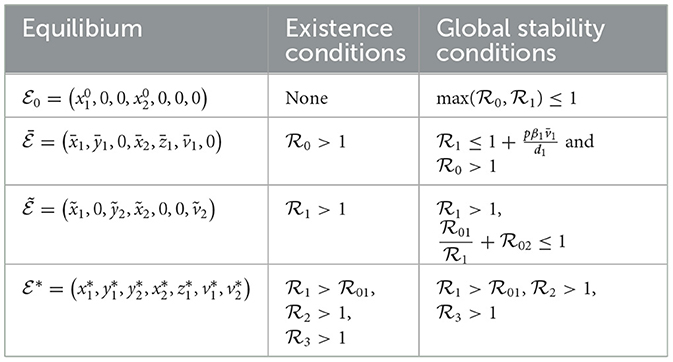
Table 2. Derivation of conditions for existence and global stability of the four equilibria.

Remark 1. An important and promising direction for future investigation involves incorporating memory effects into our model by employing fractional differential equations (FDEs) [37, 38]. Unlike classical differential equations, FDEs are particularly effective in modeling systems where the current state depends not only on present conditions but also on the history of the system–an attribute often observed in complex biological processes, including viral infections and immune responses. The intrinsic non-locality and memory-retaining nature of FDEs make them especially suitable for capturing the nuanced dynamics of HIV-HBV co-infection. In recent studies, there has been growing interest in using the Lyapunov stability theory to establish the global behavior of fractional-order systems, as highlighted in the works of [39, 40]. The Lyapunov functions introduced in this section are not only essential for the integer-order formulation of our model but also form a foundational framework that can be extended to analyze the global stability of its fractional counterpart. Such an extension would offer deeper insights into the long-term progression and control of co-infection under memory-influenced dynamics.

5 Numerical simulations

5.1 Stability of equilibria

We conduct numerical simulations for the system defined by Equations 1–7, using parameter values listed in Table 3. Some of the parameter values, as presented in Table 3, were sourced from existing literature. The rest were estimated based on plausible assumptions intended purely for illustrative and computational exploration. This was necessitated by the lack of precise clinical data, especially concerning individuals co-infected with HIV and HBV. Challenges such as ethical considerations, logistical hurdles, and small patient cohorts contribute to this data gap, making accurate parameter estimation difficult. Nevertheless, the chosen values offer a meaningful foundation for analyzing the model's qualitative dynamics and serve as a stepping stone for future research as more empirical data become available.

Table 3

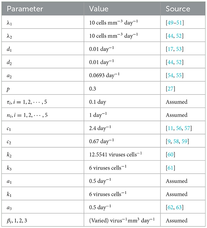
Table 3. Model parameters.

The system of delay differential equations is solved using the MATLAB solver dde23. To validate the theoretical findings discussed in earlier sections, we vary selected parameters that have a notable impact on the threshold values and, in turn, on the system's stability behavior.

To validate the results of our global stability analysis, we demonstrate that the trajectories of the system, regardless of their starting points within the biologically feasible domain, consistently evolve toward the equilibrium point that satisfies the established stability criteria. This behavior confirms that the equilibrium state dictates the system's long-term dynamics for all permissible initial conditions. Drawing methodological inspiration from the study of [41], we proceed by examining the system's response to the following representative set of initial values:

$\begin{array}{l}{x}_1(\theta )=700+10sin\theta -40k,y_1(\theta )=0.05+0.01sin\theta +0.01k,\\ y_2(\theta )=20+2sin\theta +8k,\\ x_2(\theta )=700+10sin\theta -40k,z_1(\theta )=1+0.1sin\theta +0.3k,v_1(\theta )\\ =1+0.2sin\theta +1.2k,\\ v_2(\theta )=50+3sin\theta +6k,k=1,2,\cdots ,12,\theta \in \left[-0.1,0\right].\end{array}$

To investigate the dynamical behavior of the system under varying infection pressures, we select different values for the transmission rates β₁, β₂, and β₃. These values are chosen to illustrate distinct virological scenarios, ranging from disease eradication to full co-infection. The remaining parameters are fixed as presented in Table 3. Additionally, we set τ_i = 0.1 for i = 1, 2, ⋯ , 5. We analyze four representative cases:

Case 1: Complete clearance of both infections

When the infection rates are set to β₁ = 0.0001, β₂ = 0.00002 and β₃ = 0.00003, the calculated basic reproduction numbers are ${\mathcal{R}}_0=0.10439<1$ and ${\mathcal{R}}_1=0.30682<1$. Under these conditions, the system stabilizes at the infection-free equilibrium point ${\mathcal{E}}_0=\left(1000,0,0,1000,0,0,0\right)$, which is GAS. As illustrated in Figure 2, all trajectories converge to ${\mathcal{E}}_0$, indicating that both HIV and HBV are eradicated and the uninfected hepatocytes and CD4⁺ T cells return to their normal physiological levels. This outcome confirms the theoretical results stated in Theorem 1.

Figure 2

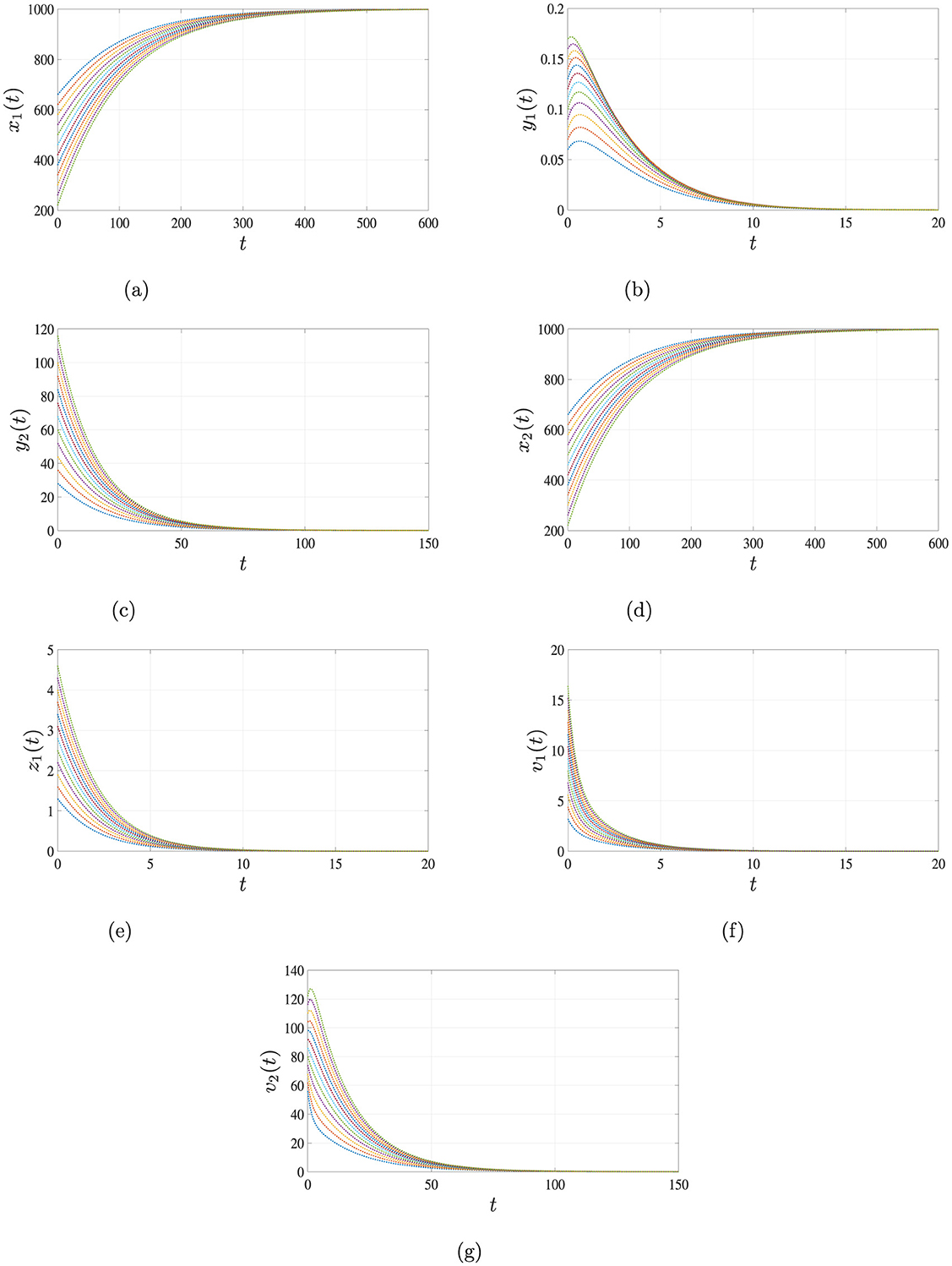
Figure 2. Simulation results for Case 1 demonstrating the global asymptotic stability of the infection-free equilibrium point ${\mathcal{E}}_0=\left(1,000,0,0,1,000,0,0,0\right)$. When the basic reproduction number satisfies ${\mathcal{R}}_C\le 1$, all trajectories of system Equations 1–7 converge to ${\mathcal{E}}_0$ over time, regardless of the initial conditions. This indicates that the infection cannot persist below this threshold. (a) Uninfected hepatocytes. (b) HIV-infected hepatocytes. (c) HBV-infected hepatocytes. (d) Uninfected CD4⁺ T cells. (e) HIV-infected CD4⁺ T cells. (f) HIV. (g) HBV.

Case 2: HIV persistence with HBV elimination

For the parameter set β₁ = 0.003, β₂ = 0.00002 and β₃ = 0.001, we obtain ${\mathcal{R}}_0=3.2749>1$ and ${\mathcal{R}}_1=0.30682<3.5470=1+\frac{p{\beta }_1{\bar{v}}_1}{d_1}$. In this scenario, only the HIV infection remains active while HBV is cleared. The solution of the system converges to the equilibrium point $\bar{\mathcal{E}}=\left(281.931,12.995,0,335.461,12.026,28.3,0\right)$, where HBV-related compartments approach zero. Figure 3 supports this outcome, which aligns with the theoretical conclusions presented in Theorem 2.

Figure 3

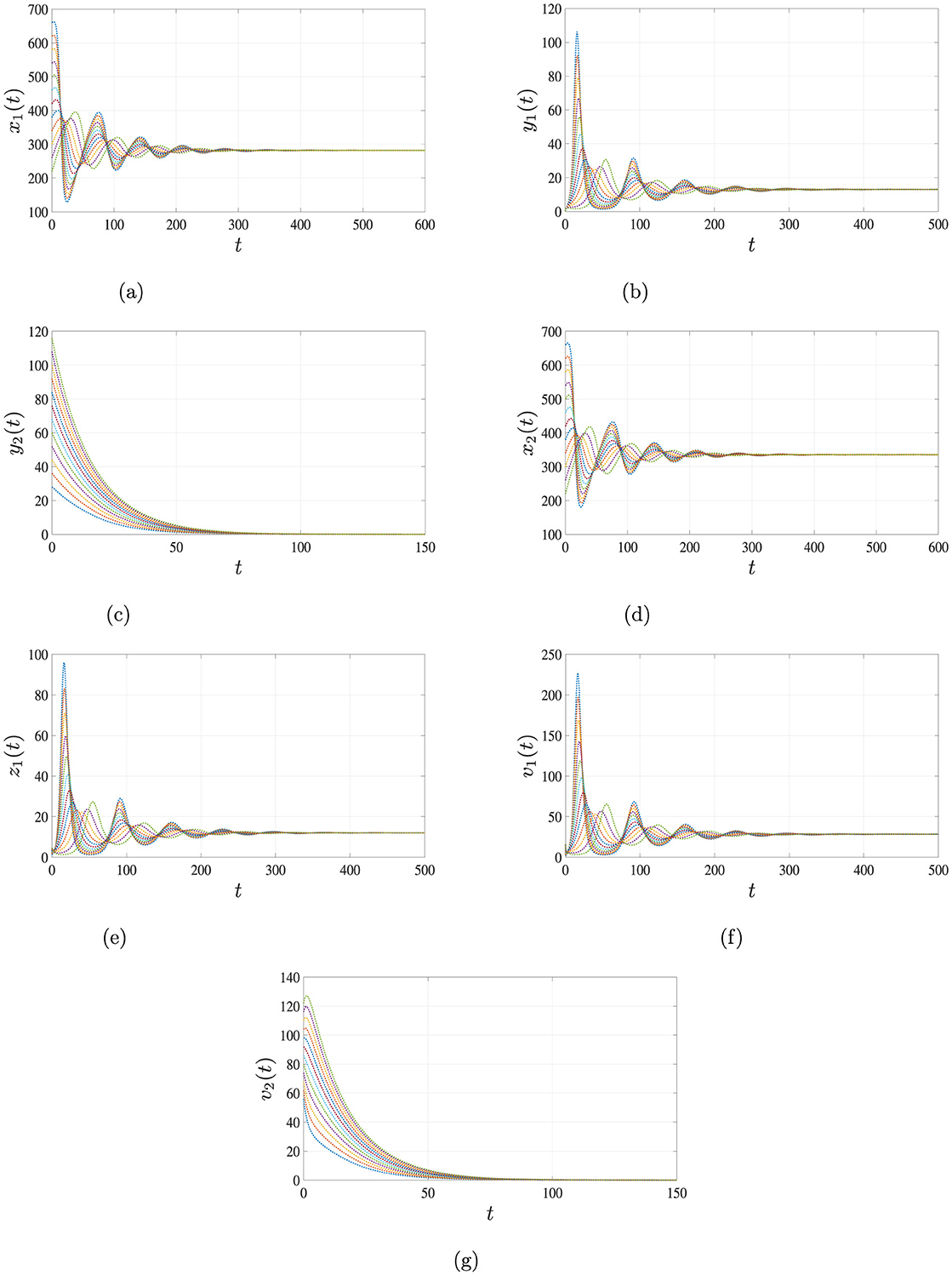
Figure 3. Simulation results for case 2 illustrating the persistence of HIV single-infection. When ${\mathcal{R}}_0>1$ and ${\mathcal{R}}_1\le 1+\frac{p{\beta }_1{\bar{v}}_1}{d_1}$ the solutions of system Equations 1–7, starting from different initial conditions, converge to the equilibrium point $\bar{\mathcal{E}}=\left(203.17,14.42,0,884.38,2.0923,18.676,0\right)$. This indicates that HIV persists in the body, while HBV is cleared over time. (a) Uninfected hepatocytes. (b) HIV-infected hepatocytes. (c) HBV-infected hepatocytes. (d) Uninfected CD4⁺ T cells. (e) HIV-infected CD4⁺ T cells. (f) HIV. (g) HBV.

Case 3: HBV persistence with HIV clearance

Choosing β₁ = 0.0017, β₂ = 0.0002, and β₃ = 0.00001 leads to ${\mathcal{R}}_0=1.0582>1$, ${\mathcal{R}}_1=3.0682>1$ and ${\mathcal{R}}_{02}+\frac{{\mathcal{R}}_{01}}{{\mathcal{R}}_1}=0.35455<1$. The system evolves toward the equilibrium $\tilde{\mathcal{E}}=\left(325.93,0,88.013,1000,0,0,103.41\right)$, indicating persistence of HBV infection and clearance of HIV. The simulation results depicted in Figure 4 validate the analytical findings of Theorem 3.

Figure 4

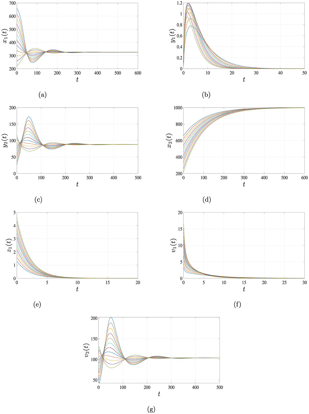
Figure 4. Simulation results for Case 3 illustrating the persistence of HBV single-infection. When ${\mathcal{R}}_1>1$ and $\frac{{\mathcal{R}}_{01}}{{\mathcal{R}}_1}+{\mathcal{R}}_{02}\le 1$, the solutions of system Equations 1–7, starting from different initial conditions, converge to the equilibrium point $\tilde{\mathcal{E}}=\left(325.93,0,88.013,1000,0,0,103.41\right)$. This indicates that HBV persists in the body, while HIV is cleared over time. (a) Uninfected hepatocytes. (b) HIV-infected hepatocytes. (c) HBV-infected hepatocytes. (d) Uninfected CD4⁺ T cells. (e) HIV-infected CD4⁺ T cells. (f) HIV. (g) HBV.

Case 4: Coexistence of HIV and HBV

Finally, for β₁ = 0.00015, β₂ = 0.0002 and β₃ = 0.001, the system exhibits a more complex dynamic with ${\mathcal{R}}_1=3.0682>{\mathcal{R}}_{01}=0.092107$, ${\mathcal{R}}_2=1.4771>1$, ${\mathcal{R}}_3=67.429>1$. In this case, both HIV and HBV persist, and the system converges to a co-infected equilibrium ${\mathcal{E}}^{*}=\left(325.93,0.18091,86.707,676.99,5.8454,6.816,101.88\right)$, which is GAS. The long-term dynamics illustrated in Figure 5 confirm the results of Theorem 4, demonstrating stable co-infection of both viruses.

Figure 5

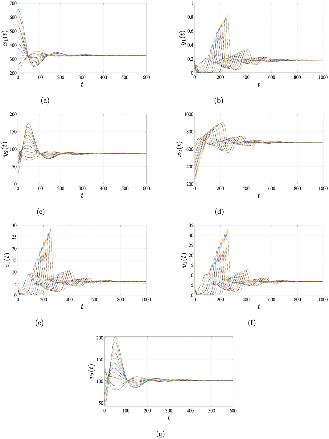
Figure 5. Simulation results for Case 4 illustrating the persistence of both HIV and HBV co-infection. When ${\mathcal{R}}_1>{\mathcal{R}}_{01}$, ${\mathcal{R}}_2>1$, and ${\mathcal{R}}_3>1$, the solutions of system Equations 1–7, starting from three distinct initial conditions, converge to the endemic equilibrium point ${\mathcal{E}}^{*}=\left(325.93,0.18091,86.707,676.99,5.8454,6.816,101.88\right)$. This indicates that both HIV and HBV persist in the body under this scenario. (a) Uninfected hepatocytes. (b) HIV-infected hepatocytes. (c) HBV-infected hepatocytes. (d) Uninfected CD4⁺ T cells. (e) HIV-infected CD4⁺ T cells. (f) HIV. (g) HBV.

The outcomes of these four scenarios clearly illustrate the significant impact of infection rate parameters on the progression and stability of the system. Varying these rates leads to distinct biological outcomes, including total clearance of both viruses, dominance of one infection, or stable coexistence of HIV and HBV. The close agreement between simulation results and analytical predictions reinforces the model's reliability in representing the intricate dynamics of HIV-HBV co-infection.

5.2 Sensitivity analysis

Sensitivity analysis aims to assess how variations in model parameters influence the system's output dynamics [42]. A common method involves calculating sensitivity indices, which quantify the proportional change in a model outcome resulting from a small change in a specific parameter. This technique is particularly useful for identifying parameters that most significantly affect the basic reproduction numbers ${\mathcal{R}}_i$, where i = 0, 1. Given that ${\mathcal{R}}_0$ and ${\mathcal{R}}_1$ are differentiable functions of key parameters, their sensitivity indices can be derived using partial derivatives [43]. In this study, we focus on computing the sensitivity indices for both ${\mathcal{R}}_0$ and ${\mathcal{R}}_1$, with the goal of understanding how different parameters contribute to the stability of the infection-free equilibrium ${\mathcal{E}}_0$. The normalized sensitivity index of ${\mathcal{R}}_i$ w.r.t. a given parameter η is given as follows [42]:

$\begin{array}{l}{S}_{\eta }^{{\mathcal{R}}_i}=\frac{\partial {\mathcal{R}}_i}{\partial \eta }\times \frac{\eta }{{\mathcal{R}}_i},i=0,1.\end{array}$

5.2.1 Sensitivity analysis of ${\mathcal{R}}_0$

To investigate how variations in model parameters affect the basic reproduction number HIV-only infection ${\mathcal{R}}_0$, we compute normalized sensitivity indices. These indices reflect the proportional change in ${\mathcal{R}}_0$ resulting from a small perturbation in a given parameter. The general formula used for this computation is based on partial derivatives of ${\mathcal{R}}_0$ with respect to each parameter.

$\begin{array}{l}{S}_{{\lambda }_1}^{{\mathcal{R}}_0}=S_{k_1}^{{\mathcal{R}}_0}=S_{{\beta }_1}^{{\mathcal{R}}_0}=-S_{d_1}^{{\mathcal{R}}_0}=\frac{{\lambda }_1{k}_{1}p{\beta }_1{F}_1{F}_4}{c_1{d}_1{\mathcal{R}}_0}\text{, }{S}_{{\lambda }_2}^{{\mathcal{R}}_0}=S_{k_3}^{{\mathcal{R}}_0}=S_{{\beta }_3}^{{\mathcal{R}}_0}\\ =-S_{d_2}^{{\mathcal{R}}_0}=\frac{{\lambda }_2{k}_3\left(1-p\right){\beta }_3{F}_3{F}_4}{c_1{d}_2{\mathcal{R}}_0},\\ S_{c_1}^{{\mathcal{R}}_0}=-1\text{, }{S}_p^{{\mathcal{R}}_0}=\frac{p\left(k_1{\beta }_1{\lambda }_1{d}_2{F}_1{F}_4-k_3{\beta }_3{\lambda }_2{d}_1{F}_3{F}_4\right)}{p{k}_1{\beta }_1{\lambda }_1{d}_2{F}_1{F}_4+\left(1-p\right)k_3{\beta }_3{\lambda }_2{d}_1{F}_3{F}_4}\text{, }{S}_{n_1}^{{\mathcal{R}}_0}\\ =S_{{\tau }_1}^{{\mathcal{R}}_0}=-n_1{\tau }_1\frac{{\lambda }_1{k}_{1}p{\beta }_1{F}_1{F}_4}{c_1{d}_1{\mathcal{R}}_0}\\ S_{n_3}^{{\mathcal{R}}_0}=S_{{\tau }_3}^{{\mathcal{R}}_0}=-n_3{\tau }_3\frac{{\lambda }_2{k}_3\left(1-p\right){\beta }_3{F}_3{F}_4}{c_1{d}_2{\mathcal{R}}_0}\text{, }{S}_{n_4}^{{\mathcal{R}}_0}=S_{{\tau }_4}^{{\mathcal{R}}_0}=-n_4{\tau }_4.\end{array}$

Using parameter values β₁ = 0.0017, β₂ = 0.0002, β₃ = 0.001, and τ_i = 0.1 for i = 1, 2, ⋯ , 5 along with the values listed in Table 3, we calculate the sensitivity indices of ${\mathcal{R}}_0$ as shown in Table 4.

Table 4

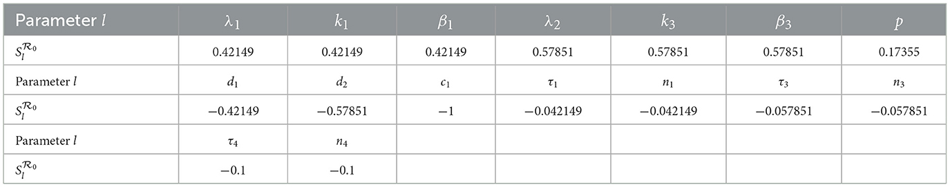
Table 4. Sensitivity of ${\mathcal{R}}_0$.

From the computed indices, we observe that parameters λ₁, k₁, β₁, λ₂, k₃, β₃, and p positively influence ${\mathcal{R}}_0$; increases in any of these raise the value of ${\mathcal{R}}_0$. On the other hand, parameters such as d₁, d₂, c₁, τ₁, n₁, τ₃, n₃, τ₄, and n₄ have a negative effect on ${\mathcal{R}}_0$, meaning that increasing them leads to a reduction in viral transmission potential.

The impact of selected parameters can be summarized as follows:

• A 10% increase in λ₁, k₁, or β₁ leads to a 4.2149% increase in ${\mathcal{R}}_0$, while the same percentage increase in λ₂, k₃, or β₃ yields a 5.7851% rise in ${\mathcal{R}}_0$.

• Conversely, increasing d₁ or d₂ by 10% results in 4.2149% and 5.7851% reductions in ${\mathcal{R}}_0$, respectively.

• A 10% rise (or drop) in the parameter c₁ results in a corresponding 10% reduction (or increase) in the value of ${\mathcal{R}}_0$.

• Parameter p has a more modest yet significant influence; a 10% increase in p increases ${\mathcal{R}}_0$ by approximately 1.7355%.

• Time-delay-related parameters such as τ₁ or n₁ impact ${\mathcal{R}}_0$ by about 4.215%, while τ₃, n₃ contribute about 5.785% each, and τ₄, n₄ account for a 10% effect.

These results indicate that ${\mathcal{R}}_0$ is especially sensitive to λ₂, k₃, β₃, p, d₂ and c₁, in agreement with biological expectations, since HIV predominantly targets CD4⁺ T cells.

5.2.2 Sensitivity analysis of ${\mathcal{R}}_1$

We now turn our attention to the basic reproduction number of HBV-only infection ${\mathcal{R}}_1$. The corresponding sensitivity indices are derived as follows: $S_{k_2}^{{\mathcal{R}}_1}=S_{{\beta }_2}^{{\mathcal{R}}_1}=S_{{\lambda }_1}^{{\mathcal{R}}_1}=-S_{c_2}^{{\mathcal{R}}_1}=-S_{d_1}^{{\mathcal{R}}_1}=1$, $S_{n_2}^{{\mathcal{R}}_1}=S_{{\tau }_2}^{{\mathcal{R}}_1}=-n_2{\tau }_2$ and $S_{n_5}^{{\mathcal{R}}_1}=S_{{\tau }_5}^{{\mathcal{R}}_1}=-n_5{\tau }_5$. Using the same parameter values as before, the calculated indices for ${\mathcal{R}}_1$ are summarized in Table 5.

Table 5

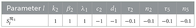
Table 5. Sensitivity of ${\mathcal{R}}_1$.

The analysis reveals that ${\mathcal{R}}_1$ is positively affected by increases in k₂, β₂, and λ₁, while it decreases with higher values of c₂ and d₁. Specifically:

• A 10% increase in k₂, β₂, or λ₁ results in a 10% increase in ${\mathcal{R}}_1$.

• A 10% increase in c₂ or d₁ leads to a 10% decrease in ${\mathcal{R}}_1$.

• Likewise, increasing τ₂ or n₂ by 100% reduces ${\mathcal{R}}_1$ by 10%, and the same applies to τ₅ and n₅

The reproduction number ${\mathcal{R}}_1$ shows no sensitivity to the remaining parameters in system (Equation 1–7), indicating that the progression of HBV infection in this model is primarily governed by a smaller subset of variables.

5.3 Co-infection dynamics of HIV and HBV under antiviral therapies

To address the impact of antiviral therapies on the progression of HIV and HBV co-infection, we modify the original system of Equations 1–7 by incorporating two pharmacological interventions:

(i) an antiretroviral drug with efficacy parameter ϵ₁∈[0, 1] targeting HIV [44], and

(ii) an anti-HBV agent with efficacy ϵ₂∈[0, 1] aimed at suppressing hepatitis B viral replication [45].

The resulting treatment-augmented model is expressed as follows:

$\begin{array}{ll}{\dot{x}}_1={\lambda }_1-d_1{x}_1-\left(1-{ϵ}_1\right)p{\beta }_1{x}_1{v}_1-\left(1-{ϵ}_2\right){\beta }_2{x}_1{v}_2,& (17)\end{array}$

$\begin{array}{ll}{\dot{y}}_1=p{F}_1{\beta }_1\left(1-{ϵ}_1\right)x_1^{{\tau }_1}{v}_1^{{\tau }_1}-a_1{y}_1,& (18)\end{array}$

$\begin{array}{ll}{\dot{y}}_2=\left(1-{ϵ}_2\right)F_2{\beta }_2{x}_1^{{\tau }_2}{v}_2^{{\tau }_2}-a_2{y}_2,& (19)\end{array}$

$\begin{array}{ll}{\dot{x}}_2={\lambda }_2-d_2{x}_2-\left(1-{ϵ}_1\right)\left(1-p\right){\beta }_3{x}_2{v}_1,& (20)\end{array}$

$\begin{array}{ll}{\dot{z}}_1=\left(1-{ϵ}_1\right)\left(1-p\right)F_3{\beta }_3{x}_2^{{\tau }_3}{v}_1^{{\tau }_3}-a_3{z}_1,& (21)\end{array}$

$\begin{array}{ll}{\dot{v}}_1=F_4[k_1{a}_1{y}_1^{{\tau }_4}+k_3{a}_3{z}_1^{{\tau }_4}]-c_1{v}_1,& (22)\end{array}$

$\begin{array}{ll}{\dot{v}}_2=k_2{a}_2{F}_5{y}_2^{{\tau }_5}-c_2{v}_2.& (23)\end{array}$

The therapeutic impact can be understood by analyzing the basic reproduction numbers for HIV and HBV in the presence of treatment. Referring to the basic reproduction numbers ${\mathcal{R}}_0$ (for HIV) and ${\mathcal{R}}_1$ (for HBV) as previously defined in Section 3.1, the modified reproduction numbers under drug action are computed as folllows:

$\begin{array}{l}{\mathcal{R}}_0^{\text{treated}}\left({ϵ}_1\right)=\frac{k_1\left(1-{ϵ}_1\right)p{\beta }_1{\lambda }_1{F}_1{F}_4}{c_1{d}_1}+\frac{k_3\left(1-{ϵ}_1\right)\left(1-p\right){\beta }_3{\lambda }_2{F}_3{F}_4}{c_1{d}_2}\\ =\left(1-{ϵ}_1\right){\mathcal{R}}_0\le {\mathcal{R}}_0,\text{and }\\ {\mathcal{R}}_1^{\text{treated}}\left({ϵ}_2\right)=\frac{k_2\left(1-{ϵ}_2\right){\beta }_2{\lambda }_1{F}_2{F}_5}{c_2{d}_1}=\left(1-{ϵ}_2\right){\mathcal{R}}_1\le {\mathcal{R}}_1.\end{array}$

To ensure long-term viral clearance, the aim is to suppress both reproduction numbers below unity:

$\begin{array}{l}{\mathcal{R}}_0^{\text{treated}}\left({ϵ}_1\right)\le 1\text{ and }{\mathcal{R}}_1^{\text{treated}}\left({ϵ}_2\right),\end{array}$

which would guarantee global asymptotic stability of the disease-free equilibrium ${\mathcal{E}}_0$.

Solving the above inequalities yields the minimum efficacies–also termed critical drug efficacies–required for viral eradication:

• ${ϵ}_1^{\mathrm{\text{cr}}}=1-\frac{1}{{\mathcal{R}}_0}$ ensuring ${\mathcal{R}}_0^{\mathrm{\text{treated}}}\left({ϵ}_1\right)\le 1$ for all ${ϵ}_1\ge {ϵ}_1^{\mathrm{\text{cr}}}$

• ${ϵ}_2^{\mathrm{\text{cr}}}=1-\frac{1}{{\mathcal{R}}_1}$ ensuring ${\mathcal{R}}_1^{\mathrm{\text{treated}}}\left({ϵ}_2\right)\le 1$ for all ${ϵ}_2\ge {ϵ}_2^{\mathrm{\text{cr}}}$

Using model parameters including β₁ = 0.00015, β₂ = 0.0002, β₃ = 0.001, τ_i = 0.1 for i = 1, 2, ⋯ , 5, along with values from Table 3, we compute the following thresholds:

• ${ϵ}_1^{\mathrm{\text{cr}}}\simeq 0.34421$

• ${ϵ}_2^{\mathrm{\text{cr}}}\simeq 0.6741$

The results provided in Figures 6, 7 can be interpreted as follows.

Figure 6

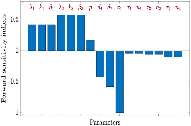
Figure 6. Sensitivity analysis for ${\mathcal{R}}_0$.

Figure 7

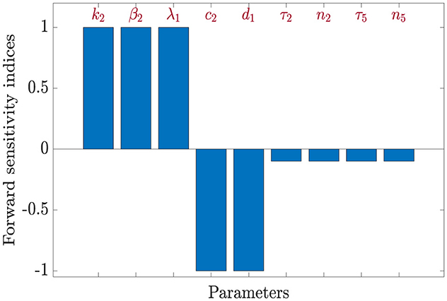
Figure 7. Sensitivity analysis for ${\mathcal{R}}_1$.

(i) If ϵ₁ ≥ 0.34421 ≤ ≤ 1 and ϵ₂ ≥ 0.67407, both HIV and HBV infections are effectively controlled, and the system stabilizes at the disease-free state ${\mathcal{E}}_0$ (GAS).

(ii) If ϵ₁ < 0.34421 and/or ϵ₂ < 0.67407, then at least one reproduction number exceeds 1, causing the infection-free equilibrium to lose stability. In such cases, a chronic infection equilibrium may emerge and become globally attractive.

To further analyze therapeutic outcomes, we simulate the model system (Equations 17–23) under varying drug efficacies, employing the following set of initial functions for θ ∈ [−0.1, 0]:

$\begin{array}{l}{x}_1(\theta )=750+10sin\theta ,y_1(\theta )=0.5+0.1sin\theta ,y_2(\theta )=30+3sin\theta ,\\ x_2(\theta )=800+10sin\theta ,z_1(\theta )=2+0.1sin\theta ,v_1(\theta )=3+0.1sin\theta ,\\ v_2(\theta )=50+3sin\theta .\end{array}$

We examine a range of ϵ₁ and ϵ₂ values as detailed in Table 6.

Table 6

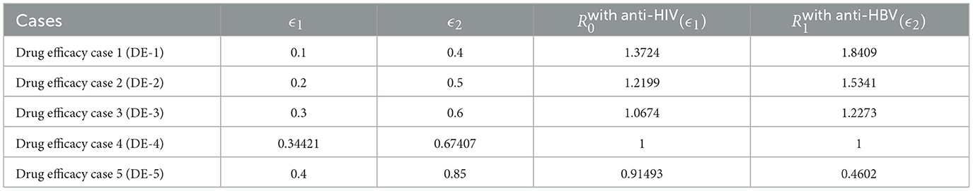
Table 6. Impact of drug efficacies ϵ₁ and ϵ₂ on ${\mathcal{R}}_0^{\mathrm{\text{with anti-HIV}}}\left({ϵ}_1\right)$ and ${\mathcal{R}}_1^{\mathrm{\text{with anti-HBV}}}\left({ϵ}_2\right)$.

Simulation outcomes, summarized in Table 6 and illustrated in Figure 8, reveal that increasing antiviral efficacies leads to a marked decline in both ${\mathcal{R}}_0^{\mathrm{\text{treated}}}$ and ${\mathcal{R}}_1^{\mathrm{\text{treated}}}$. This pharmacodynamic effect contributes to the restoration of healthy hepatocyte and CD4⁺ T cell populations, while infected compartments (e.g., y₁, y₂, z₁) and viral loads (v₁, v₂) decrease accordingly.

Figure 8

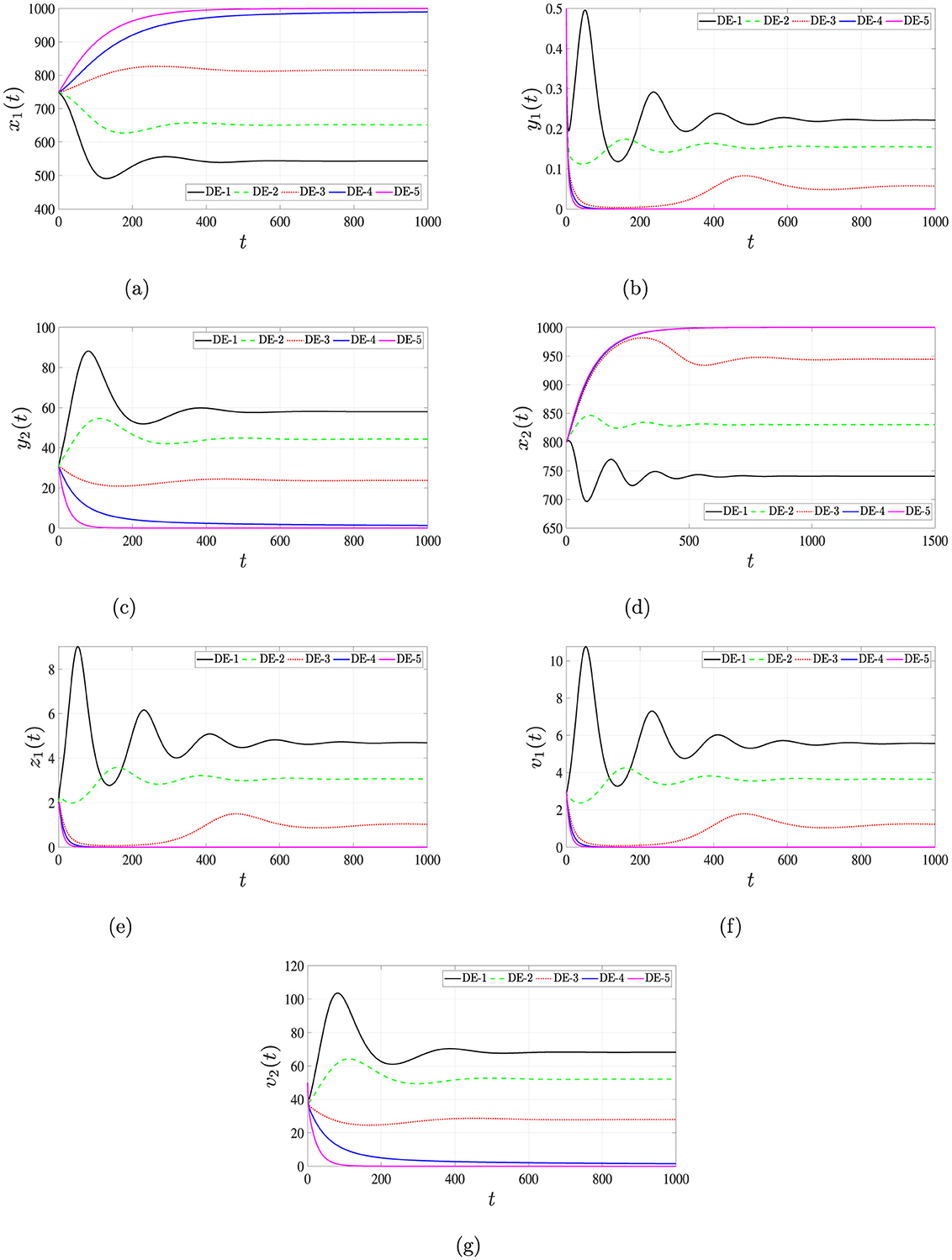
Figure 8. Solutions of system (Equations 16–22) for different antiviral effectiveness rates, ϵ₁ and ϵ₂. (a) Uninfected hepatocytes. (b) HIV-infected hepatocytes. (c) HBV-infected hepatocytes. (d) Uninfected CD4⁺ T cells. (e) HIV-infected CD4⁺ T cells. (f) HIV. (g) HBV.

These findings highlight the critical role of treatment efficacy in shifting the system dynamics toward recovery, emphasizing the need for optimal dosing strategies to achieve viral suppression and potential eradication. The analysis demonstrates that when antiviral drug efficacies exceed specific threshold values, the basic reproduction numbers fall below one, leading the system toward a globally stable, infection-free equilibrium. This underscores the importance of well-calibrated therapeutic interventions in effectively controlling and potentially eliminating HIV and HBV co-infections.

The set of equations defined by Equations 17–23 can be viewed through the framework of a nonlinear control system, in which the parameters ϵ₁ and ϵ₂ represent controllable inputs corresponding to the efficacies of anti-HIV and anti-HBV therapies, respectively. By treating these drug efficacies as control variables, we can employ tools from optimal control theory to determine treatment strategies that minimize viral loads and optimize patient outcomes [46–48]. This approach enables the systematic design of therapeutic protocols for individuals co-infected with HIV and HBV, ensuring both effectiveness and efficiency in long-term disease management.

5.3.1 Influence of time delays on the dynamics of HIV-HBV co-infection

Among the various time delay parameters influencing the system dynamics, it has been observed that the basic reproduction number ${\mathcal{R}}_0$ is most sensitive to variations in the delay parameter τ₄ (maturation delay of newly released HIV), while ${\mathcal{R}}_1$ is similarly influenced by the delay τ₅ (maturation delay of newly released HBV). Given this sensitivity, our analysis will focus on assessing how delays τ₄ and τ₅ affect the co-dynamics of HIV and HBV.

Using the transmission rate parameters β₁ = 0.00015, β₂ = 0.0002 and β₃ = 0.001, along with other parameter values specified in Table 3, we fix τ₁ = τ₂ = τ₃ = 0.01 and vary τ₄ and τ₅ to explore their impact on the stability of the disease-free equilibrium point ${\mathcal{E}}_0$. Since the expressions for ${\mathcal{R}}_0$ and ${\mathcal{R}}_1$ explicitly incorporate τ₄ and τ₅, respectively, any modification in these delays will directly affect the stability characteristics of ${\mathcal{E}}_0$. Notably, increasing either τ₄ or τ₅ tends to reduce the corresponding reproduction number, thus potentially promoting system stability.

The initial conditions for the delay differential system (Equation 1–7) are defined over the interval θ ∈ [−4, 0] as:

$\begin{array}{l}{x}_1(\theta )=850+10sin\theta ,y_1(\theta )=0.5+0.1sin\theta ,y_2(\theta )=25+3sin\theta ,\end{array}$

$\begin{array}{l}{x}_2(\theta )=800+10sin\theta ,z_1(\theta )=25+2sin\theta ,v_1(\theta )=15+0.5sin\theta ,\end{array}$

$\begin{array}{l}{v}_2(\theta )=15+0.6sin\theta .\end{array}$

To determine the threshold values of τ₄ and τ₅ that ensure global asymptotic stability of the infection-free state, we express the reproduction numbers as functions of these delays:

$\begin{array}{l}{\mathcal{R}}_0\left({\tau }_4\right)=e^{-n_4{\tau }_4}\left(\frac{k_{1}p{\beta }_1{\lambda }_1{e}^{-n_1{\tau }_1}}{c_1{d}_1}+\frac{k_3\left(1-p\right){\beta }_3{\lambda }_2{e}^{-n_3{\tau }_3}}{c_1{d}_2}\right),\\ {\mathcal{R}}_1\left({\tau }_5\right)=e^{-n_5{\tau }_5}\frac{k_2{\beta }_2{\lambda }_1{e}^{-n_2{\tau }_2}}{c_2{d}_1}.\end{array}$

To guarantee that ${\mathcal{R}}_0\left({\tau }_4\right)\le 1$ and ${\mathcal{R}}_1\left({\tau }_5\right)\le 1$, we compute the critical values ${\tau }_4^{cr}$ and ${\tau }_5^{cr}$ as:

$\begin{array}{l}{\tau }_4^{cr}=max\left\{0,\frac{1}{n_4}ln\left(\frac{k_{1}p{\beta }_1{\lambda }_1{e}^{-n_1{\tau }_1}}{c_1{d}_1}+\frac{k_3\left(1-p\right){\beta }_3{\lambda }_2{e}^{-n_3{\tau }_3}}{c_1{d}_2}\right)\right\},\\ {\tau }_5^{cr}=max\left\{0,\frac{1}{n_5}ln\left(\frac{k_2{\beta }_2{\lambda }_1{e}^{-n_2{\tau }_2}}{c_2{d}_1}\right)\right\}.\end{array}$

Substituting the parameter values from Table 3, we obtain the numerical approximations: ${\tau }_4^{cr}\simeq 0.61192$ and ${\tau }_5^{cr}\simeq 1.3111$. Therefore:

• If ${\tau }_4^{cr}\ge 0.61192$ and ${\tau }_5^{cr}\ge 1.3111$, then both ${\mathcal{R}}_0\left({\tau }_4\right)\le 1$ and ${\mathcal{R}}_1\left({\tau }_5\right)\le 1$, ensuring that the infection-free equilibrium ${\mathcal{E}}_0$ is GAS.

• Conversely, if ${\tau }_4^{cr}<0.61192$ or ${\tau }_5^{cr}<1.3111$, the corresponding reproduction number(s) exceed 1, destabilizing ${\mathcal{E}}_0$ and possibly rendering another equilibrium globally attractive.

As observed in Table 7, increasing the delays τ₄ and τ₅ leads to a reduction in the reproductive numbers ${\mathcal{R}}_0\left({\tau }_4\right)$ and ${\mathcal{R}}_1\left({\tau }_5\right)$. Figure 9 presents the simulation outcomes for the full system, demonstrating the profound influence of time delays on the system dynamics. Increasing the delay durations τ₄ and τ₅ enhances the populations of uninfected hepatocytes and CD4⁺ T cells, while simultaneously decreasing the concentrations of infected cells and viral loads. This dynamic underscores the biological relevance of incorporating intracellular delays in modeling, as they exhibit effects analogous to therapeutic interventions.

Table 7

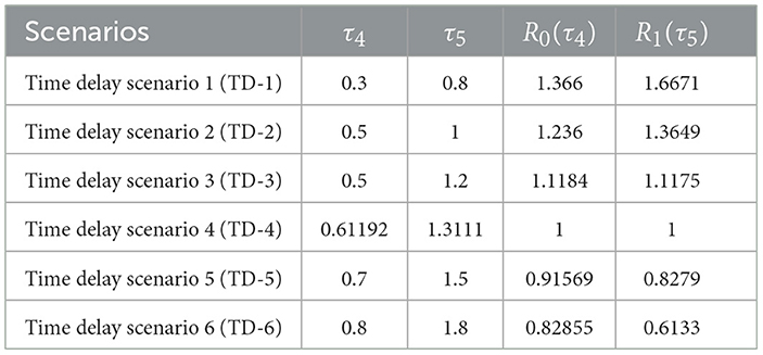
Table 7. Effect of time delays τ₄ and τ₅ on ${\mathcal{R}}_0\left({\tau }_4\right)$ and ${\mathcal{R}}_1\left({\tau }_5\right)$.

Figure 9

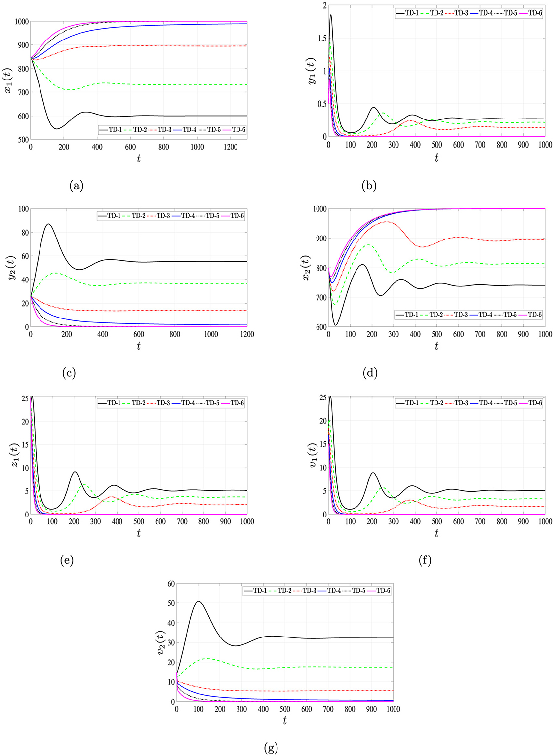
Figure 9. Solutions of system (Equation 1–7) for different time delays, τ₄ and τ₅. (a) Uninfected hepatocytes. (b) HIV-infected hepatocytes. (c) HBV-infected hepatocytes. (d) Uninfected CD4⁺ T cells. (e) HIV-infected CD4⁺ T cells. (f) HIV. (g) HBV.

In summary, incorporating biologically realistic time delays into the model not only changes the system's qualitative behavior but also offers insights into the development of novel therapies aimed at extending these delays. Such treatments could help slow down virus-cell interactions and prolong the maturation period of viruses released from infected cells. This, in turn, could significantly contribute to controlling the progression of viral activity within the host and enhancing the elimination of viruses from the body.

6 Conclusions

This study develops a mathematical model describing the within-host co-infection dynamics of HIV and HBV. In this framework, HBV primarily infects hepatocytes, while HIV targets both CD4⁺ T lymphocytes and hepatocytes. The system is represented by seven nonlinear delay differential equations (DDEs), which account for the interactions among uninfected hepatocytes, hepatocytes infected with either HIV or HBV, uninfected CD4⁺ T lymphocytes, HIV-infected CD4⁺ T lymphocytes, and free viral particles of both HIV and HBV. Two distinct delays are incorporated into the model: one representing the latency in cell infection and the other reflecting the maturation period of newly produced virions. The model ensures that all solutions are biologically feasible, remaining non-negative and bounded over time. Four equilibrium states are identified, and corresponding threshold quantities ${\mathcal{R}}_i$ (for i = 0, 1, 2, 3) are derived to characterize their behavior. Conditions guaranteeing the global asymptotic stability of each equilibrium point are established using Lyapunov function techniques along with LaSalle's invariance principle. We performed numerical simulations and sensitivity analysis to validate the theoretical findings and to determine the most effective parameters on the basic reproduction numbers for HIV-only (${\mathcal{R}}_0$) and HBV-only (${\mathcal{R}}_1$) infections. We also studied the effects of two types of antiviral treatments: one for HIV and the other for HBV. We calculated the minimum treatment efficacy needed for clearing the virus from the body. Furthermore, we studied the effect of time delays on the dynamics of viral co-infection and found that these delays reduce the basic reproduction numbers. This highlights the role and importance of considering time delays in modeling viral co-infection, as neglecting these delays leads to an overestimation of the drug's efficacy required to clear the virus. It is also noted that longer delays show effects similar to antiviral therapy, which gives some insight into the idea that finding a treatment that extends the time delay period indicates a potential therapeutic benefit. These insights underscore the importance of incorporating time delays into treatment models and may contribute to the development of more effective strategies for managing coinfection.

The proposed model is capable of capturing a range of clinically observed scenarios such as

• Individuals who successfully avoid infection.

• Cases involving HIV infection alone.

• Cases involving HBV infection alone.

• Chronic co-infection with both HIV and HBV.

This framework also highlights the significant role of antiviral treatments in restoring immune competence and preserving liver function. Mathematical modeling of HIV-HBV co-infection at the within-host level has enhanced our understanding of how these viruses interact and influence disease progression. It also supports the optimization of therapeutic approaches tailored to individual patient needs.

The findings of this study contribute meaningfully to the clinical management of HIV-HBV co-infections. By identifying thresholds for treatment effectiveness and outlining conditions that lead to viral clearance or persistence, this study aids in refining treatment strategies, guiding personalized care and improving patient outcomes. Additionally, these insights can support broader public health efforts aimed at mitigating the long-term burden of co-infections.

Data availability statement

The raw data supporting the conclusions of this article will be made available by the authors, without undue reservation.

Author contributions

AE: Conceptualization, Formal analysis, Writing – original draft, Writing – review & editing. AA: Formal analysis, Investigation, Methodology, Writing – original draft, Writing – review & editing. AH: Formal analysis, Investigation, Methodology, Writing – original draft, Writing – review & editing.

Funding

The author(s) declare that no financial support was received for the research and/or publication of this article.

Conflict of interest

The authors declare that the research was conducted in the absence of any commercial or financial relationships that could be construed as a potential conflict of interest.

Generative AI statement

The author(s) declare that no Gen AI was used in the creation of this manuscript.

Publisher's note

All claims expressed in this article are solely those of the authors and do not necessarily represent those of their affiliated organizations, or those of the publisher, the editors and the reviewers. Any product that may be evaluated in this article, or claim that may be made by its manufacturer, is not guaranteed or endorsed by the publisher.

Supplementary material

The Supplementary Material for this article can be found online at: https://www.frontiersin.org/articles/10.3389/fams.2025.1633039/full#supplementary-material

References

1. Corcorran MA, Kim HN. Chronic hepatitis B and HIV coinfection. Topics Antiviral Med. (2023) 31:14.

Google Scholar

2. Weldemhret L. Epidemiology and challenges of HBV/HIV co-infection amongst HIV-infected patients in endemic areas. HIV/AIDS-Res Palliat Care. (2021) 13:485–490. doi: 10.2147/HIV.S273649

PubMed Abstract | Crossref Full Text | Google Scholar

3. Ullah MA, Raza N, Omame A, Alqarni MS. A new co-infection model for HBV and HIV with vaccination and asymptomatic transmission using actual data from Taiwan. Physica Scripta. (2024) 99:065254. doi: 10.1088/1402-4896/ad4b6c

Crossref Full Text | Google Scholar

4. Wodarz D, Levy DN. Human immunodeficiency virus evolution towards reduced replicative fitness in vivo and the development of AIDS. Proc Biol Sci. (2007) 274:2481–91. doi: 10.1098/rspb.2007.0413

PubMed Abstract | Crossref Full Text | Google Scholar

5. Zerbato JM, Avihingsanon A, Singh KP, Zhao W, Deleage C, Rosen E., et al. HIV DNA persists in hepatocytes in people with HIV-hepatitis B co-infection on antiretroviral therapy. Bullet Mathem Biol. (2023) 87:104391. doi: 10.1016/j.ebiom.2022.104391

PubMed Abstract | Crossref Full Text | Google Scholar

6. Blackard JT, Sherman KE. HCV/HIV co-infection: time to re-evaluate the role of HIV in the liver? J Viral Hepatitis. (2008) 15:323–30. doi: 10.1111/j.1365-2893.2008.00970.x

PubMed Abstract | Crossref Full Text | Google Scholar

7. Seeger C, Mason WS. Hepatitis B virus biology, microbiology and molecular. Biol Rev. (2000) 64:51–68. doi: 10.1128/MMBR.64.1.51-68.2000

PubMed Abstract | Crossref Full Text | Google Scholar

8. Nowak MA, Bangham CRM. Population dynamics of immune responses to persistent viruses. Science. (1996) 272:74–9. doi: 10.1126/science.272.5258.74

PubMed Abstract | Crossref Full Text | Google Scholar

9. Nowak MA, Bonhoeffer S, Hill AM, Boehme R, Thomas HC, McDade H. Viral dynamics in hepatitis B virus infection. Proc Natl Acad Sci U S A. (1996) 93:4398–402. doi: 10.1073/pnas.93.9.4398

PubMed Abstract | Crossref Full Text | Google Scholar

10. Lv L, Yang J, Hu Z, Fan D. Dynamics analysis of a delayed HIV model with latent reservoir and both viral and cellular infections. Mathem Methods Appl Sci. (2025) 48:6063–80. doi: 10.1002/mma.10655

Crossref Full Text | Google Scholar

11. Culshaw RV, Ruan S. A delay-differential equation model of HIV infection of CD4⁺ T-cells. Mathem Biosci. (2000) 165:27–39. doi: 10.1016/S0025-5564(00)00006-7

PubMed Abstract | Crossref Full Text | Google Scholar

12. Prakash S, Umrao AK, Srivastava PK. Bifurcation and stability analysis of within host HIV dynamics with multiple infections and intracellular delay. Chaos. (2025) 35:013128. doi: 10.1063/5.0232978

PubMed Abstract | Crossref Full Text | Google Scholar

13. Hmarrass H, Qesmi R. Global stability and Hopf bifurcation of a delayed HIV model with macrophages, CD4+ T cells with latent reservoirs and immune response. Eur Phys J Plus. (2025) 140:335. doi: 10.1140/epjp/s13360-025-06001-z

Crossref Full Text | Google Scholar

14. Rathnayaka NS, Wijerathna JK, Pradeep GSA. Stability properties and hopf bifurcation of a delayed HIV dynamics model with saturation functional response, absorption effect and cure rate. Int J Analy Appl. (2025) 23:92–92. doi: 10.28924/2291-8639-23-2025-92

Crossref Full Text | Google Scholar

15. Chen C, Ye Z, Zhou Y. Stability and Hopf bifurcation of a cytokine-enhanced HIV infection model with saturation incidence and three delays. Int J Bifurcat Chaos. (2024) 34:2450133. doi: 10.1142/S0218127424501335

Crossref Full Text | Google Scholar

16. Hu Z, Yang J, Li Q, Liang S, Fan D. Mathematical analysis of stability and Hopf bifurcation in a delayed HIV infection model with saturated immune response. Mathem Methods Appl Sci. (2024) 47:9834–57. doi: 10.1002/mma.10097

Crossref Full Text | Google Scholar

17. Gourley SA, Kuang Y, Nagy JD. Dynamics of a delay differential equation model of hepatitis B virus infection. J Biol Dynam. (2008) 2:140–53. doi: 10.1080/17513750701769873

PubMed Abstract | Crossref Full Text | Google Scholar

18. Foko S Dynamical analysis of a general delayed HBV infection model with capsids and adaptive immune response in presence of exposed infected hepatocytes. J Mathem Biol. (2024) 88:75. doi: 10.1007/s00285-024-02096-7

PubMed Abstract | Crossref Full Text | Google Scholar

19. Prakash M, Rakkiyappan R, Manivannan A, Zhu H, Cao J. Stability and bifurcation analysis of hepatitis B-type virus infection model. Mathem Methods Appl Sci. (2021) 44:6462–81. doi: 10.1002/mma.7198

Crossref Full Text | Google Scholar

20. Chen C, Zhou Y, Ye Z, Gu M. Stability and Hopf bifurcation of a HBV infection model with capsids and CTL immune response delay. Eur Phys J Plus. (2024) 139:1–22. doi: 10.1140/epjp/s13360-024-05764-1

Crossref Full Text | Google Scholar

21. Bowong S, Kamganga J, Tewa J, Tsanou B. Modelling and analysis of hepatitis B and HIV co-infections. In: Proceedings of the 10th African Conference on Research in Computer Science and Applied Mathematics. At Yamoussoukro, Ivory Cost (2010). p. 109–16.

Google Scholar

22. Endashaw EE, Mekonnen TT. Modeling the effect of vaccination and treatment on the transmission dynamics of hepatitis B virus and HIV/aids coinfection. J Appl Mathemat. (2022) 2022:5246762. doi: 10.1155/2022/5246762

PubMed Abstract | Crossref Full Text | Google Scholar

23. Endashaw EE, Gebru DM, Alemneh HT. Coinfection dynamics of HBV-HIV/AIDS with mother-to-child transmission and medical interventions. Comput Mathem Methods Med. (2022) 2022:4563577. doi: 10.1155/2022/4563577

Crossref Full Text | Google Scholar

24. Rasheed A, Raza A, Omame A. Analysis of a novel mathematical model for HBV and HIV incorporating vertical transmission and intervention measures. Model Earth Syst Environm. (2025) 11:222. doi: 10.1007/s40808-025-02408-w

Crossref Full Text | Google Scholar

25. Teklu SW. Workie AH. HIV/AIDS and HBV co-infection with optimal control strategies and cost-effectiveness analyses using integer order model. Sci Rep. (2025) 15:4004. doi: 10.1038/s41598-024-83442-z

PubMed Abstract | Crossref Full Text | Google Scholar

26. Abebaw YF, Teklu SW. Dynamical analysis of HIV/AIDS and HBV co-infection model with drug-related kidney disease using optimal control theory. Model Earth Syst Environm. (2025) 11:1–34. doi: 10.1007/s40808-024-02203-z

Crossref Full Text | Google Scholar

27. Nampala H, Luboobi LS, Mugisha JY, Obua C, Jablonska-Sabuka M. Modelling hepatotoxicity and antiretroviral therapeutic effect in HIV/HBV co-infection. Mathem Biosci. (2018) 302:67–79. doi: 10.1016/j.mbs.2018.05.012

PubMed Abstract | Crossref Full Text | Google Scholar

28. Nampala H, Jablonska-Sabuka M, Singull M. Mathematical analysis of the role of HIV/HBV latency in hepatocytes. J Appl Mathem. (2021) 2021:5525857. doi: 10.1155/2021/5525857

Crossref Full Text | Google Scholar

29. Herz AV, Bonhoeffer S, Anderson RM, May RM, Nowak MA. Viral dynamics in vivo: limitations on estimates of intracellular delay and virus decay. Proc Natl Acad Sci. (1996) 93:7247–51. doi: 10.1073/pnas.93.14.7247

PubMed Abstract | Crossref Full Text | Google Scholar

30. Hale JK, Verduyn M, Lunel S. Introduction to Functional Differential Equations. New York: Springer-Verlag. (1993).

Google Scholar

31. Kuang Y. Delay Differential Equations: With Applications in Population Dynamics. Cambridge, MA: Academic Press (1993).

Google Scholar

32. Van den Driessche P, Watmough J. Reproduction numbers and sub-threshold endemic equilibria for compartmental models of disease transmission. Mathem Biosci. (2002) 180:29–48. doi: 10.1016/S0025-5564(02)00108-6

PubMed Abstract | Crossref Full Text | Google Scholar

33. Korobeinikov A Global properties of basic virus dynamics models. Bullet Mathem Biol. (2004) 66:879–83. doi: 10.1016/j.bulm.2004.02.001

PubMed Abstract | Crossref Full Text | Google Scholar

34. Barbashin EA. Introduction to the Theory of Stability. Groningen: Wolters-Noordhoff (1970).

Google Scholar

35. LaSalle JP. The Stability of Dynamical Systems. Philadelphia: SIAM (1976).

Google Scholar

36. Lyapunov AM. The General Problem of the Stability of Motion. London: Taylor & Francis, Ltd. (1992). doi: 10.1080/00207179208934253

Crossref Full Text | Google Scholar

37. Yaseen RM, Ali NF, Mohsen AA, Khan A, Abdeljawad T. The modeling and mathematical analysis of the fractional-order of Cholera disease: Dynamical and simulation. Partial Differ Equ Appl Math. (2024) 12:100978. doi: 10.1016/j.padiff.2024.100978

Crossref Full Text | Google Scholar

38. Hattaf K, A new mixed fractional derivative with applications in computational biology. Computation. (2024) 12:7. doi: 10.3390/computation12010007

Crossref Full Text | Google Scholar

39. Yaagoub Z, Sadki M, Allali K. A generalized fractional hepatitis B virus infection modelwith both cell-to-cell and virus-to-cell transmissions. Nonlinear Dynam. (2024) 112:16559–85. doi: 10.1007/s11071-024-09867-3

PubMed Abstract | Crossref Full Text | Google Scholar

40. Naim M, Zeb A, Mohsen AA, Sabbar Y, Yıldız M. Local and global stability of a fractional viral infection model with two routes of propagation, cure rate and non-lytic humoral immunity. Mathem Model Numer Simul Appl. (2024) 4:94–115. doi: 10.53391/mmnsa.1517325

Crossref Full Text | Google Scholar

41. Song B, Zhang Y, Sang Y. Zhang L. Stability and Hopf bifurcation on an immunity delayed HBV/HCV model with intra-and extra-hepatic coinfection and saturation incidence. Nonlinear Dynam. (2023) 111:14485–511. doi: 10.1007/s11071-023-08580-x

Crossref Full Text | Google Scholar

42. Chitnis N, Hyman JM, Cushing JM. Determining important parameters in the spread of malaria through the sensitivity analysis of a mathematical model. Bullet Mathem Biol. (2008) 70:1272–96. doi: 10.1007/s11538-008-9299-0

PubMed Abstract | Crossref Full Text | Google Scholar

43. Marino S, Hogue IB, Ray CJ, Kirschner DE. A methodology for performing global uncertainty, sensitivity analysis in systems biology. J Theor Biol. (2008) 254:178–96. doi: 10.1016/j.jtbi.2008.04.011

PubMed Abstract | Crossref Full Text | Google Scholar

44. Callaway DS, Perelson AS. HIV-1 infection and low steady state viral loads. Bullet Mathem Biol. (2002) 64:29–64. doi: 10.1006/bulm.2001.0266

PubMed Abstract | Crossref Full Text | Google Scholar

45. Lewin SR, Ribeiro RM, Walters T, Lau GK, Bowden S, Locarnini S, Perelson AS. Analysis of hepatitis B viral load decline under potent therapy: complex decay profiles observed. Hepatology. (2001) 34:1012–20. doi: 10.1053/jhep.2001.28509

PubMed Abstract | Crossref Full Text | Google Scholar

46. Joshi HR Optimal control of an HIV immunology model. Optim Control Appl Methods. (2002) 23:199–213. doi: 10.1002/oca.710

Crossref Full Text | Google Scholar

47. Mohsen AA, Naji RK. Dynamical analysis within-host and between-host for HIV/AIDS with the application of optimal control strategy. Iraqi J Sci. (2020) 61:1173–89. doi: 10.24996/ijs.2020.61.5.25

PubMed Abstract | Crossref Full Text | Google Scholar

48. Nampala H, Jabłońska-Sabuka M, Singull M. Analysis of HIV therapy in the liver using optimal control and pharmacokinetics. J Mathem Indust. (2025) 15:2. doi: 10.1186/s13362-025-00167-y

Crossref Full Text | Google Scholar

49. Wodarz D. Hepatitis C. virus dynamics and pathology: the role of CTL and antibody responses. J General Virol. (2003) 84:1743–50. doi: 10.1099/vir.0.19118-0

PubMed Abstract | Crossref Full Text | Google Scholar

50. Wodarz D. Mathematical models of immune effector responses to viral infections: Virus control versus the development of pathology. J Comput Appl Mathem. (2005) 184:301–19. doi: 10.1016/j.cam.2004.08.016

Crossref Full Text | Google Scholar

51. Webster G, Reignat S, Maini M, Whalley S, Ogg G, King A, et al. Incubation phase of acute hepatitis B in man: Dynamic of cellular immune mechanisms. Hepatology. (2000) 32:1117–24. doi: 10.1053/jhep.2000.19324

PubMed Abstract | Crossref Full Text | Google Scholar

52. Mohri H, Bonhoeffer S, Monard S, Perelson AS, Ho DD. Rapid turnover of T lymphocytes in SIV-infected rhesus macaques. Science. (1998) 279:1223–7. doi: 10.1126/science.279.5354.1223

PubMed Abstract | Crossref Full Text | Google Scholar

53. Dahari H, Lo A, Ribeiro R, Perelson A. Modeling hepatitis C virus dynamics: liver regeneration and critical drug efficacy. J Theoret Biol. (2007) 247:371–81. doi: 10.1016/j.jtbi.2007.03.006

PubMed Abstract | Crossref Full Text | Google Scholar

54. Eikenberry S, Hews S, Nagy JD, Kuang Y. The dynamics of a delay model of hepatitis B virus infection with logistic hepatocyte growth. Mathem Biosci Eng. (2009) 6:283–99. doi: 10.3934/mbe.2009.6.283

PubMed Abstract | Crossref Full Text | Google Scholar

55. Yousfi N, Hattaf K, Tridane A. Modeling the adaptive immune response in HBV infection. J Mathem Biol. (2011) 63:933–57. doi: 10.1007/s00285-010-0397-x

PubMed Abstract | Crossref Full Text | Google Scholar

56. Perelson AS, Kirschner DE, De Boer R. Dynamics of HIV infection of CD4+ T cells. Mathem Biosci. (1993) 114:81–125. doi: 10.1016/0025-5564(93)90043-A

PubMed Abstract | Crossref Full Text | Google Scholar

57. Wang Y, Zhou Y, Wu J, Heffernan J. Oscillatory viral dynamics in a delayed HIV pathogenesis model. Mathem Biosci. (2009) 219:104–12. doi: 10.1016/j.mbs.2009.03.003

PubMed Abstract | Crossref Full Text | Google Scholar

58. Tsiang M, Rooney J, Toole J, Gibbs C. Biphasic clearance kinetics of hepatitis B virus from patients during adefovir dipivoxil therapy. Hepatology. (1999) 29:1863–9. doi: 10.1002/hep.510290626

PubMed Abstract | Crossref Full Text | Google Scholar

59. Ciupe SM, Ribeiro RM, Nelson PW, Perelson AS. Modeling the mechanisms of acute hepatitis B virus infection. J Theor Biol. (2007) 247:23–35. doi: 10.1016/j.jtbi.2007.02.017

PubMed Abstract | Crossref Full Text | Google Scholar

60. Harroudi S, Meskaf A, Allali K. Modelling the adaptive immune response in HBV infection model with HBV DNA-containing capsids. Differ Equ Dyn Syst. (2023) 31:371–93. doi: 10.1007/s12591-020-00549-1

Crossref Full Text | Google Scholar

61. Manna K Global properties of a HBV infection model with HBV DNA-containing capsids and CTL immune response. Int J Appl Comput Mathem. (2017) 3:2323–38. doi: 10.1007/s40819-016-0205-4

Crossref Full Text | Google Scholar

62. Shih Y, Liu C. Hepatitis C virus and hepatitis B virus co-infection. Viruses. (2020) 12:1–11. doi: 10.3390/v12070741

PubMed Abstract | Crossref Full Text | Google Scholar

63. Manna K, Chakrabarty S. Chronic hepatitis B infection and HBV DNA-containing capsids: modeling and analysis. Commun Nonlinear Sci Numer. (2015) 22:383–95. doi: 10.1016/j.cnsns.2014.08.036

PubMed Abstract | Crossref Full Text | Google Scholar